Meta-Learner for Amharic Sentiment Classification


Abstract
:1. Introduction
- The provision of an annotated data sets [22].
- The effect of SMOTE with TF-IDF character n-grams feature is tested on Amharic sentiment classification by using ensemble learning.
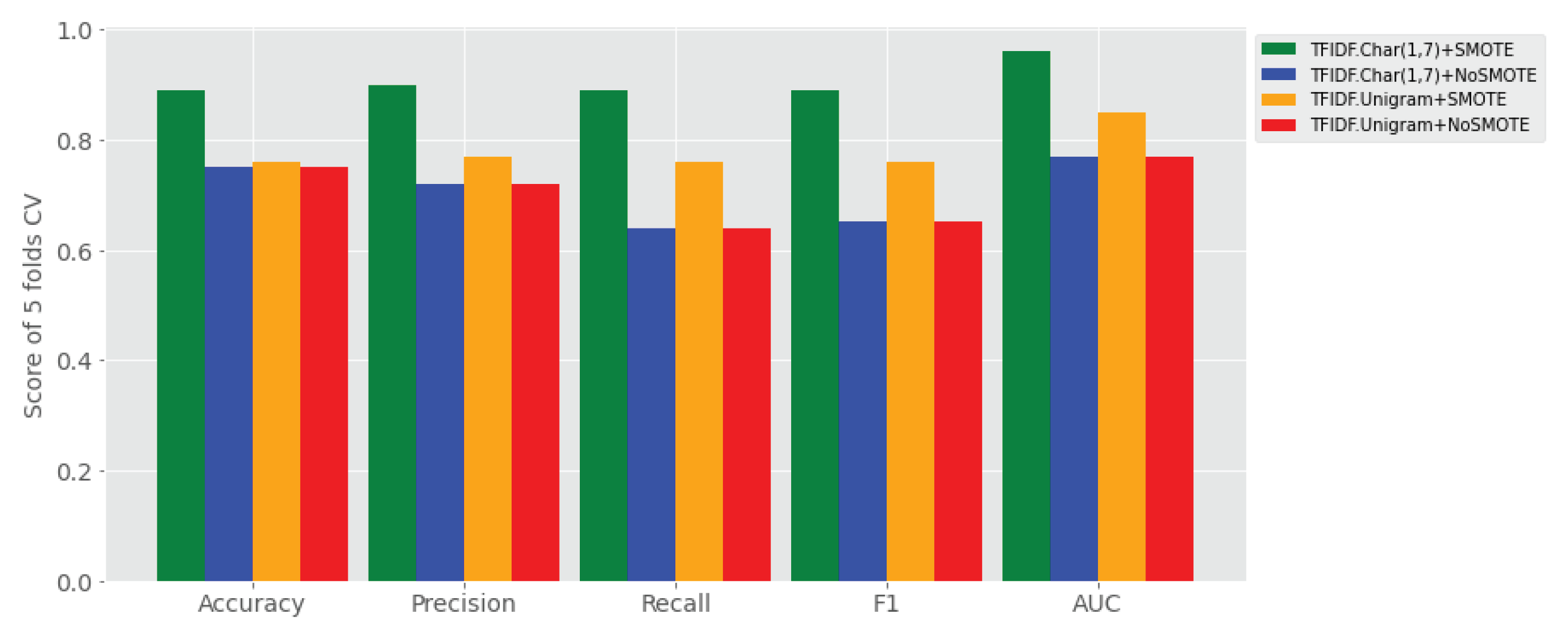
- SMOTE with TF-IDF character n-grams feature works better than the one with (or without) SMOTE on performance of Amharic sentiment classification of user generated text.
- SMOTE with TF-IDF word uni-gram has shown performance gains of sentiment classification as compared to TF-IDF uni-gram with no SMOTE and
- TF-IDF character (1,7) grams is found to be the most salient feature for discriminating sentiment categories of Amharic user-generated text.
2. Literature Review
2.1. Feature Selection
2.2. Imbalanced Learning
2.3. Ensemble Approaches for Sentiment Classification
3. Materials and Methods
3.1. Overview
3.2. Evaluation Metrics
- (i) True Positive (TP) is the number of samples belonging to the positive class that are correctly predicted by the model.
- (ii) True Negative (TN) is the number of samples belonging to the negative class that are correctly predicted by the model.
- (iii) False Positive (FP) is the number of samples belonging to the positive classes that are wrongly predicted by the model. This is also called Type I Error.
- (iv) False Negative (FN) is the number of samples belonging to the negative classes that are wrongly predicted by the model. This is also called Type II Error.
- (i) Accuracy (A) is the percentage of correctly predicted samples, i.e.,
- (ii) Precision (P) is the evaluation metric that measures the correctly predicted samples actually turned out to be positive, i.e.,Note that precision is a metric that measures the reliability of the model.
- (iii) Recall (R) is a measure of the number of actual positive samples which are correctly predicted by the model, i.e.,Recall is also called sensitivity. Note that precision is more important to tell when the model predicted more false positive samples than false negative samples. In contrast, recall is a more important metric to tell if the model predicts more false negative than false positive samples.
- (iv) F1-Score (F1) is the harmonic mean between precision and recall. It is calculated from precision and recall, i.e.,
- (v) Area Under Curve(AUC) is the most popular evaluation metric for binary classification problem. AUC is a measure of the probability of a classifier that will rank a randomly chosen positive example higher than a randomly chosen negative example. AUC ranges [0,1], the higher the AUC implies, the better the model.
- (vi) Logarithmic Loss (LogLoss) is used to measure how close or far model’s predicted value from actual value. For the binary classification problem, LogLoss is also called binary cross-entropy, which is the negative average of the log of corrected predicted probabilities. For N samples, LogLoss is given bywhere is the actual value, is the probability of class 1, and is the probability of class 0.
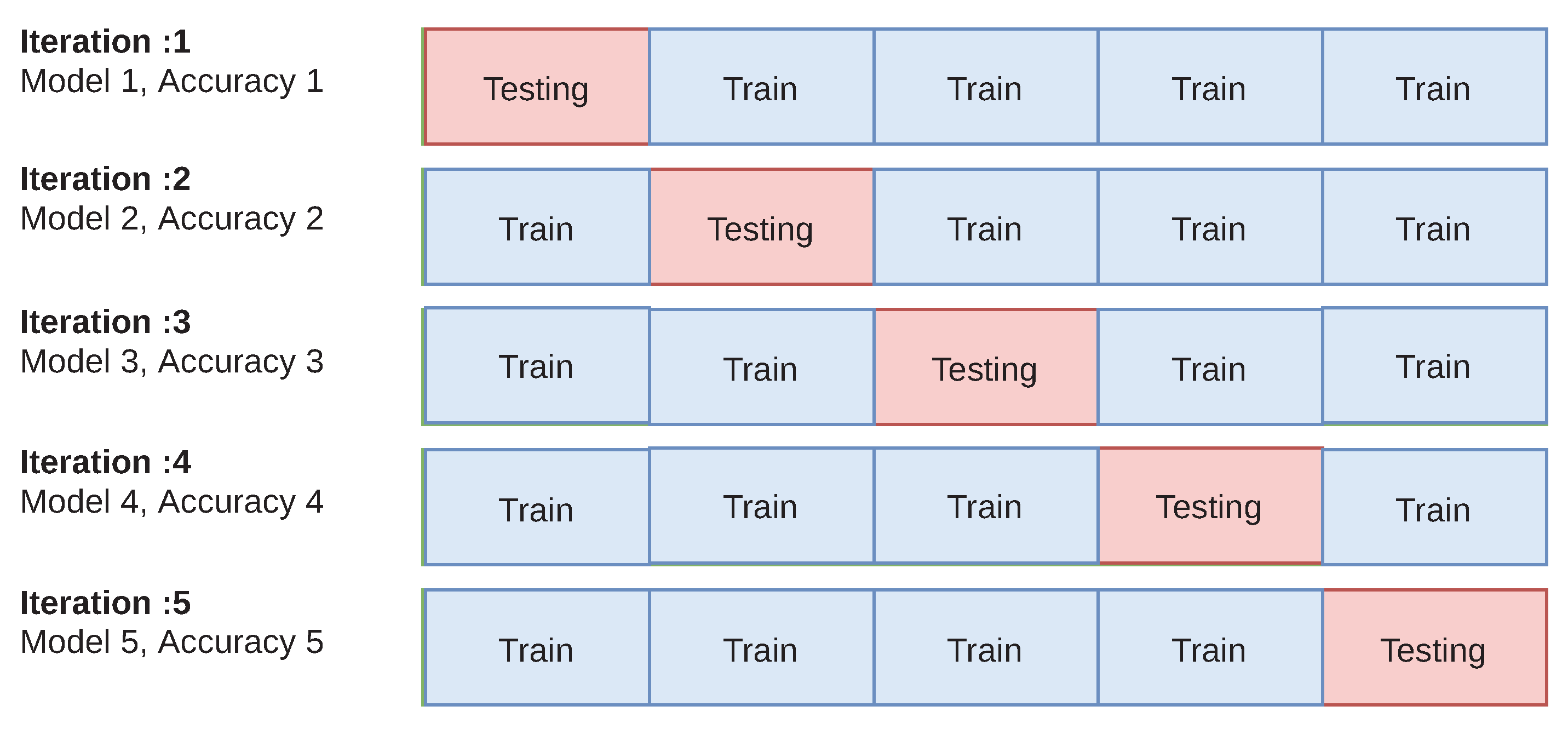
- (vii) Cross-Validation (CV): K-fold Cross-Validation is the model evaluation technique where all data set samples are randomly divided into k folds of equal size. As there is no standard rule for selecting k, usually the value of K is 5 or 10. We chose K = 5. For each run, K-1 folds are used for training the model and the remaining are used as the testing set. This is repeated k times so that each of the folds is used once for testing. The average accuracy of the 5 models and standard deviation is returned. This is illustrated in Figure 1.The benefits of using cross-validation include (i) its capability of avoiding overfitting/underfitting, (ii) it can evaluate model consistency by producing accuracy/error rate for all the test sets, and (iii) it has also capability of training/testing on a small data by using the total datasets [47].
- (viii) Mean of Accuracy and Standard Deviation (SD): Note that from statistics, ‘mean’ is defined as the average of accuracy of the models in five folds using testing sets, whereas ‘variance’ is the sum of the squares of the model’s accuracy deviated from the mean divided by the total number of models. Larger standard deviation shows that the prediction of a model is more sensitive to future observations, and vice versa.
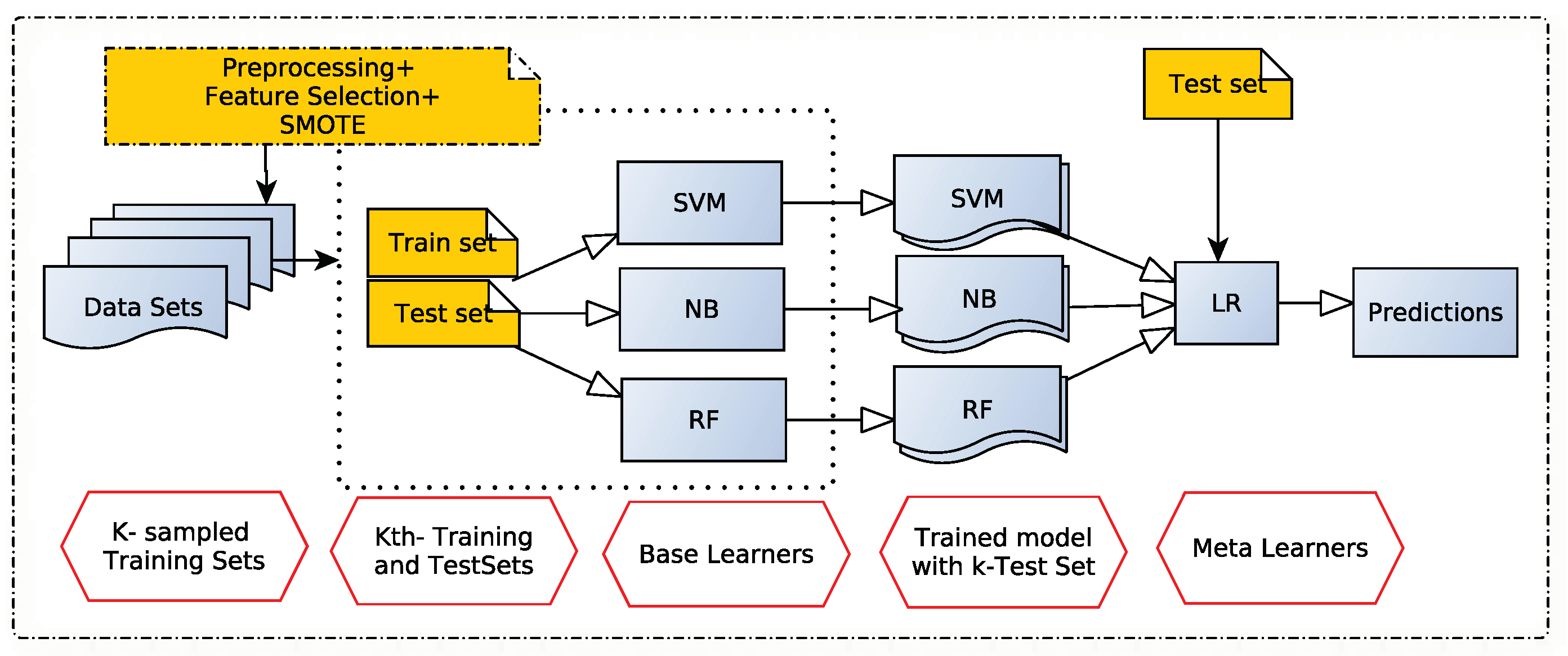
3.3. Proposed Stacking Algorithm
| Algorithm 1: Proposed Ensemble Learning. |
| Input: Labeled Data Set |
| Output: Average Accuracy of Trained Meta-learner Model M |
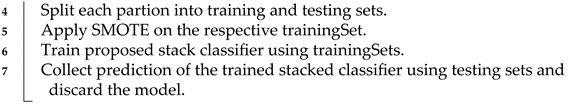
|
4. Results and Discussions
4.1. Experimental Settings
4.2. Results
4.3. Discussions
5. Conclusions
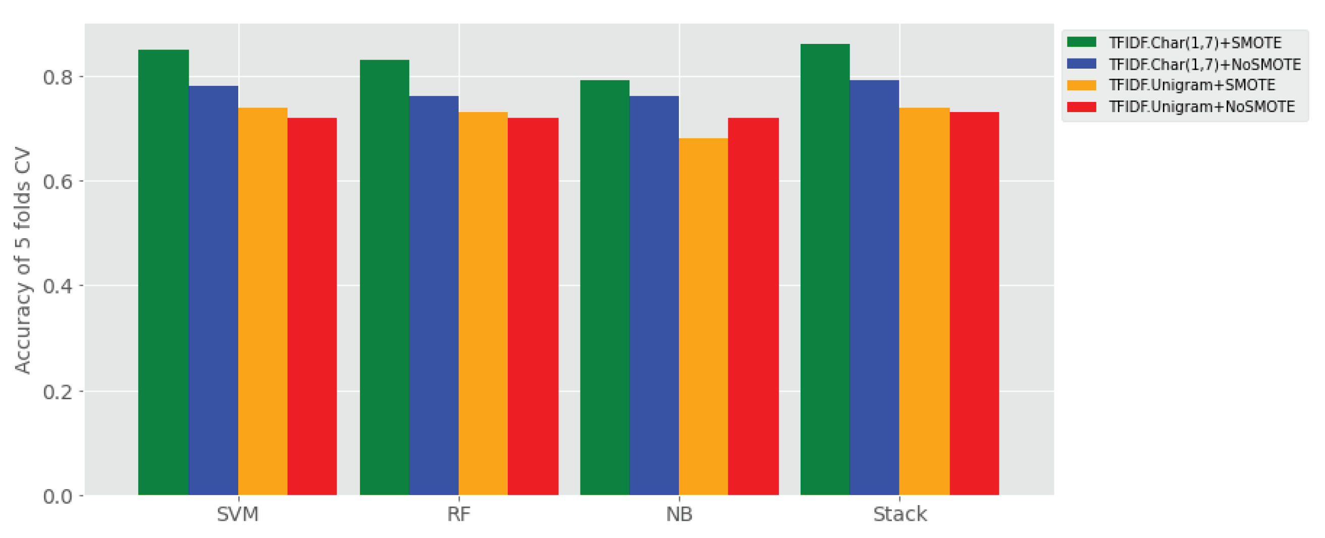
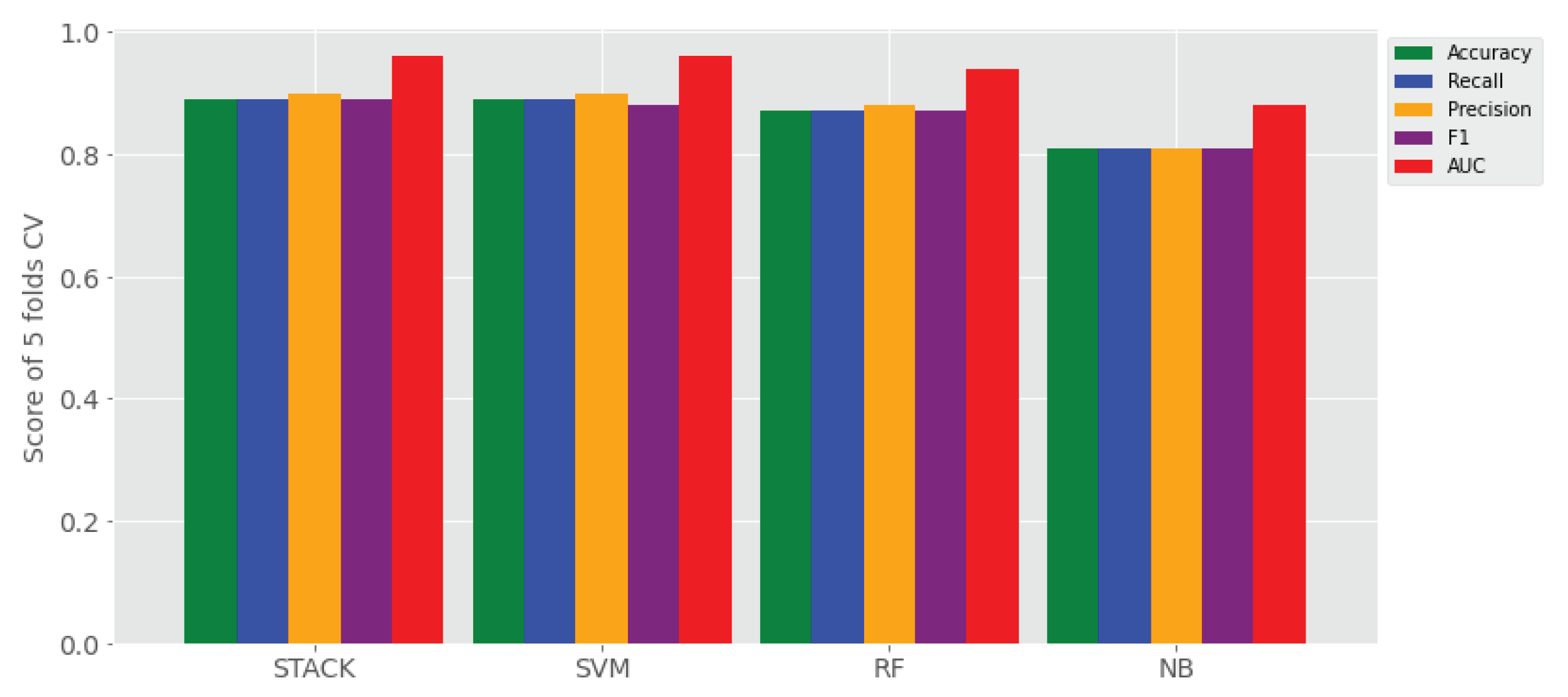
- (1) To what extent does ensemble learning improve Amharic sentiment classification on a small set of user-generated texts compared to base learners? The answer for this research question is reported all four experimental settings (i.e., Experiment I–IV), where its results are reported in Table 4. That means, the proposed stack ensemble model outperforms the individual learners on all sentiment classification data sets using TF-IDF character (1, 7) gram with and without application of SMOTE shown in Table 4, as compared to the data sets using TF-IDF uni-gram with and without SMOTE balancing technique. The proposed stack learner has achieved a rise of accuracy ranging from 10% to 31% over all base learners in the above experimental settings.
- (2) Which feature representation (TF-IDF uni-gram, TF-IDF character n-grams) has better performance of Amharic sentiment classification with the proposed ensemble approach? The answer for this research question is provided in Table 4 that reveals ensemble learner outperforms on TF-IDF character n-grams over TF-IDF word uni-gram.
- (3) Does SMOTE technique improve performance of the proposed approach by balancing the imbalanced labeled user generated data? The answer to this research question is reported in Table 4, where SMOTE has significantly improved sentiment classification of ensemble learners and base learners when it is applied with both TF-IDF character n-grams and TF-IDF word uni-gram feature sets.
- (4) On which feature representation of Amharic texts does SMOTE show higher performance improvement of sentiment classification? The answer is provided in Table 4 showing that SMOTE boosts sentiment classification when it applied to TF-IDF character n-grams.
Author Contributions
Funding
Institutional Review Board Statement
Informed Consent Statement
Data Availability Statement
Conflicts of Interest
Abbreviations
| BERT | Bidirectional Encoder Representations from Transformers |
| CNN | Convolutional Neural Network |
| CV | Cross-Validation |
| DT | Decision Tree |
| EBC | Ethiopian Broadcasting Corporate |
| GCOA | Government Communication Office Affair |
| KNN | K-Nearest Neighbor |
| LSTM | Long Short-Term Memory |
| LR | Logistic Regression |
| ME | Maximum Entropy |
| MPQA | Multi-Perspective Question Answering |
| NB | Naive Bayes |
| NTUSD | National Taiwan University Semantic Dictionary |
| PMO | Prime Minister Office |
| RF | Random Forest |
| SD | Standard Deviation |
| SVM | Support Vector Machine |
| SMOTE | Synthetic Minority Oversampling Technique |
| TF-IDF | Term Frequency-Inverse Document Frequency |
References
- Ruder, S.; Korashy, H. The 4 Biggest Open Problems in NLP. Ain Shams Eng. J. Available online: https://ruder.io/4-biggest-open-problems-in-nlp/ (accessed on 2 March 2021).
- Palmer, A. Computational Linguistics for Low-Resource Languages. Slide Presentation, Saarland University, Saarbrücken, Germany. Available online: http://www.coli.uni-saarland.de/courses/CL4LRL (accessed on 2 October 2020).
- Lam, K.; Al Tarouti, F.; Kalita, J. Creating Lexical Resources For Endangered Languages. In Proceedings of the 2014 Workshop on the Use of Computational Methods in the Study of Endangered Languages, Baltimore, ML, USA, 26 June 2014; pp. 54–62. [Google Scholar]
- Janse, M. Language Death And Language Maintenance: Problems And Prospects. In Language Death and Language Maintenance: Theoretical, Practical And Descriptive Approaches; Janse, M., Tol, S., Eds.; John Benjamins: Amsterdam, The Netherlands, 2003; pp. 9–17. [Google Scholar] [CrossRef]
- King, B. Practical Natural Language Processing for Low-Resource Languages. Ph.D. Thesis, Department of Computer Science, University of Michigan, Michigan, MI, USA, 2015. [Google Scholar]
- Gebremeskel, S. Sentiment Mining Model for Opinionated Amharic Texts. Master’s Thesis, Department of Computer Science, Addis Ababa University, Addis Ababa, Ethiopia, 2010. [Google Scholar]
- Tilahun, T. Linguistic localization of opinion mining from Amharic blogs. Int. J. Inf. Technol. Comput. Sci. Perspect. 2014, 3, 890. [Google Scholar]
- Alemneh, G.N.; Rauber, A.; Atnafu, S. Dictionary Based Amharic Sentiment Lexicon Generation. In Proceedings of the International Conference on Information and Communication Technology for Development for Africa, Bahir Dar, Ethiopia, 28–30 May 2019; pp. 311–326. [Google Scholar] [CrossRef]
- Alemneh, G.N.; Rauber, A.; Atnafu, S. Corpus based Amharic sentiment lexicon generation. In Proceedings of the SA Forum for Artificial Intelligence Research, Published at CEUR Workshop Proceedings (CEUR-WS.org), Cape Town, South Africa, 3–6 December 2019. [Google Scholar]
- Philemon, W.; Mulugeta, W. A Machine Learning Approach to Multi-Scale Sentiment Analysis of Amharic Online Posts. HiLCoE J. Comput. Sci. Technol. 2014, 2, 8. [Google Scholar]
- Dessalew, C. Public Sentiment Analysis for Amharic News. Master’s Thesis, Bahir Dar University, Bahir Dar, Ethiopia, 2019. [Google Scholar]
- Mihret, M.; Atinaf, M. Sentiment Analysis Model for Opinionated Awngi Text. In Proceedings of the African Conference (AFRICON), Accra, Ghana, 25 September 2019; pp. 1–6. [Google Scholar] [CrossRef]
- Tsegaw, M. Sarcasm Detection for Amharic Text. Master’s Thesis, Bahir Dar University, Bahir Dar, Ethiopia, 2020. [Google Scholar]
- Alemu, Y. Deep Learning Approach For Amharic Sentiment Analysis. Master’s Thesis, University of Gondar, Gonder, Ethiopia, 2018. [Google Scholar]
- Fikre, T. Effect of Preprocessing on Long Short Term Memory-based Sentiment Analysis for Amharic Language. Master’s Thesis, Addis Ababa University, Addis Ababa, Ethiopia, 2020. [Google Scholar]
- Neshir, G.; Atnafu, S.; Rauber, A. BERT Fine-Tuning for Amharic Sentiment Classification. In Proceedings of the Workshop RESOURCEFUL Co-Located with the Eighth Swedish Language Technology Conference (SLTC), University of Gothenburg, Gothenburg, Sweden, 25 November 2020. [Google Scholar]
- He, Y.; Harith, A.; Zhou, D. Exploring English Lexicon Knowledge For Chinese Sentiment Analysis. In Proceedings of the Canadian Information Processing Society (CIPS)-SIGHAN Joint Conference on Chinese Language Processing, Beijing, China, 28–29 August 2010. [Google Scholar]
- Opitz, D.; Maclin, R.; Brown, D. Popular ensemble methods: An empirical study. J. Artif. Intell. Res. 1999, 11, 169–198. [Google Scholar] [CrossRef]
- Ganaie, M.A.; Hu, M.; Tanveer, M.; Suganthan, P.N. Ensemble deep learning: A review. arXiv 2021, arXiv:2104.02395. [Google Scholar]
- Brownlee, J. A Gentle Introduction to Ensemble Learning Algorithms. Available online: https://machinelearningmastery.com/tour-of-ensemble-learning-algorithms/ (accessed on 25 May 2021).
- Ensemble Methods: Combining Multiple Models to Improve the Desired Results. Corporate Finance Institute. Available online: https://corporatefinanceinstitute.com/resources/knowledge/other/ensemble-methods/ (accessed on 25 May 2021).
- Alemneh, G.N.; Rauber, A.; Atnafu, S. Negation Handling for Amharic Sentiment Classification. In Proceedings of the 4th Widening Natural Language Processing Workshop, Seattle, WA, USA, 8 January 2020; pp. 4–6. [Google Scholar] [CrossRef]
- Hofmann, M.; Chisholm, A. Text Mining and Visualization: Case Studies Using Open-Source Tools; CRC Press: Boca Raton, FL, USA, 2016. [Google Scholar]
- Veres, C.; Kapustin, P.; Veres, C. Enhancing Subword Embeddings with Open n-grams. In Natural Language Processing and Information Systems; NLDB 2020, Lecture Notes in Computer Science; Métais, E., Meziane, F., Horacek, H., Cimiano, P., Eds.; Springer: Berlin, Germany, 2020; Volume 12089, pp. 3–15. ISBN 978-3-030-51309-2. [Google Scholar] [CrossRef]
- Graovac, J.; Kovačević, J.; Pavlović-Lažetić, G. Language Independent n-gram-based Text Categorization with Weighting Factors: A Case Study. J. Inf. Data Manag. 2015, 6, 4. [Google Scholar]
- Piskorski, J.; Jacquet, G. TF-IDF Character n-grams versus Word Embedding-based Models for Fine-grained Event Classification: A Preliminary Study. In Proceedings of the Workshop on Automated Extraction of Socio-political Events from News, Marseille, France, 11–16 May 2020; pp. 26–34. [Google Scholar]
- Kruczek, J.; Kruczek, P.; Kuta, M. Are n-gram Categories Helpful in Text Classification? In Computational Science—ICCS 2020; Lecture Notes in Computer Science; Krzhizhanovskaya, V.V., Závodszky, G., Lees, M.H., Dongarra, J.J., Sloot, P.M.A., Brissos, S., Teixeira, J., Eds.; Springer: Berlin, Germany, 2020; pp. 524–537. ISBN 978-3-030-50416-8. [Google Scholar] [CrossRef]
- Thai-Nghe, N.; Gantner, Z.; Schmidt-Thieme, L. Cost-sensitive Learning Methods for Imbalanced Data. In Proceedings of the 2010 International Joint Conference On Neural Networks (IJCNN), Barcelona, Spain, 18–23 July 2010; pp. 1–8. [Google Scholar]
- Padurariu, C.; Breaban, M. Dealing with Data Imbalance in Text Classification. Procedia Comput. Sci. 2019, 159, 736–745. [Google Scholar] [CrossRef]
- Gonzalez-Cuautle, D.; Hernandez-Suarez, A.; Sanchez-Perez, G.; Toscano-Medina, L.; Portillo-Portillo, J.; Olivares-Mercado, J.; Perez-Meana, H.; Sandoval-Orozco, A. Synthetic Minority Oversampling Technique for Optimizing Classification Tasks in Botnet and Intrusion Detection System Datasets. Appl. Sci. 2020, 10, 794. [Google Scholar] [CrossRef] [Green Version]
- Ah-Pine, J.; Soriano-Morales, E. A Study of Synthetic Oversampling for Twitter Imbalanced Sentiment Analysis. In Proceedings of the Workshop on Interactions Between Data Mining and Natural Language Processing (DMNLP), Riva del Garda, Italy, 23 September 2016. [Google Scholar]
- Khalid, M.; Ashraf, I.; Mehmood, A.; Ullah, S.; Ahmad, M.; Choi, G. GBSVM: Sentiment Classification from Unstructured Reviews Using Ensemble Classifier. Appl. Sci. 2020, 10, 2788. [Google Scholar] [CrossRef] [Green Version]
- Wang, G.; Sun, J.; Ma, J.; Xu, K.; Gu, J. Sentiment Classification: The Contribution of Ensemble Learning. Decis. Support Syst. 2014, 57, 77–93. [Google Scholar] [CrossRef]
- Wan, Y.; Gao, Q. An Ensemble Sentiment Classification System of Twitter Data for Airline Services Analysis. In Proceedings of the International Conference On Data Mining Workshop (ICDMW), Atlantic City, AC, USA, 14–17 November 2015; pp. 1318–1325. [Google Scholar] [CrossRef]
- Alnashwan, R.; O’Riordan, A.; Sorensen, H.; Hoare, C. Improving Sentiment Analysis through Ensemble Learning of Meta-level Features. In Proceedings of the 2nd International Workshop on Knowledge Discovery on the WEB, Cagliari, Italy, 8–10 September 2016; p. 1748. [Google Scholar]
- Omar, N.; Al-Moslmi, M.; Al-Shabi, A.Q.; Al-Moslmi, T. Ensemble of Classification Algorithms for Subjectivity and Sentiment Analysis of Arabic Customers’ Reviews. Int. J. Adv. Comput. Technol. 2013, 5, 77. [Google Scholar]
- Kennedy, A.; Inkpen, D. Sentiment Classification of Movie Reviews Using Contextual Valence Shifters. Comput. Intell. 2006, 22, 110–125. [Google Scholar] [CrossRef] [Green Version]
- Tribhuvan, P.; Bhirud, S.; Deshmukh, R. Stacking Ensemble Model for Polarity Classification in Feature Based Opinion Mining. Indian J. Comput. Sci. Eng. 2018, 9. [Google Scholar] [CrossRef]
- Hassan, A.; Abbasi, A.; Zeng, D. Twitter Sentiment Analysis: A bootstrap ensemble framework. In Proceedings of the International Conference on Social Computing, Alexandria, VA, USA, 8–14 September 2013; pp. 357–364. [Google Scholar]
- Artinez-Cámara, E.; Martín-Valdivia, M.; Molina-González, M.; Perea-Ortega, J. Integrating Spanish Lexical Resources by Meta-classifiers For Polarity Classification. J. Inf. Sci. 2014, 40, 538–554. [Google Scholar] [CrossRef]
- Sagi, O.; Rokach, L. Advanced Review Ensemble learning: A survey. WIREs Data Min. Knowl. Discov. 2018, 8, e1249. [Google Scholar] [CrossRef]
- Zhou, Z. Ensemble Methods: Foundations and Algorithms; Chapman: Orange, CA, USA, 2019. [Google Scholar]
- Mujtaba, H. Ensemble Learning with Stacking and Blending. Mygreatlearning. Available online: https://www.mygreatlearning.com/blog/ensemble-learning-with-stacking-and-blending/ (accessed on 23 April 2021).
- Singh, J.; Singh, G.; Singh, R. Optimization of sentiment analysis using machine learning classifiers. Hum. Cent. Comput. Inf. Sci. 2017, 7. [Google Scholar] [CrossRef]
- Raschka, S. Python Machine Learning Unlock Deeper Insights into Machine Learning with this Vital Guide to Cutting-Edge Predictive Analytics; Packt Publishing: Birmingham, UK, 2015; p. 456. [Google Scholar]
- Raschka, S. MLxtend: Providing Machine Learning and Data Science Utilities and Extensions to Python Scientific Computing Stack. J. Open Source Softw. 2018, 3, 638. [Google Scholar] [CrossRef]
- Badvelu, J. Cross-Validation for Classification Models. Analytics. Vidhya. Available online: https://medium.com/analytics-vidhya/cross-validation-for-classification-models-9bb6506dee00 (accessed on 12 October 2020).
- ZEMENTV. Sparks Film Production. Available online: https://www.youtube.com/channel/UCzfrWFpc5sgVyybMHp5b5sQ (accessed on 14 February 2021).
- GCAO Ethiopia. Available online: https://www.facebook.com/gcao.ethiopia (accessed on 12 May 2019).
- Office of the Prime Minister-Ethiopia. Available online: https://www.facebook.com/PMOEthiopia/ (accessed on 25 May 2020).
- Ethiopian Broadcasting Corporation. Available online: https://www.facebook.com/EBCzena (accessed on 2 June 2020).
- Kelemework, W. Automatic Amharic Text News Classification: A Neural Networks Approach. Ethiop. J. Sci. Technol. 2013, 6, 127–137. [Google Scholar]
- Scikit-Learn Machine Learning in Python. Available online: https://scikit-learn.org/stable/ (accessed on 2 June 2019).
- Rezapour, M. Sentiment classification of skewed shoppers’ reviews using machine learning techniques, examining the textual features. Eng. Rep. 2021, 3, e12280. [Google Scholar] [CrossRef]
- Chawla, N.; Bowyer, K.; Hall, L.; Kegelmeyer, W. SMOTE: Synthetic Minority Over-sampling Technique. J. Artif. Intell. Res. 2002, 16, 321–357. [Google Scholar] [CrossRef]
- Kowsari, K.; Jafari Meimandi, K.; Heidarysafa, M.; Mendu, S.; Barnes, L.; Brown, D. Text Classification Algorithms: A Survey. Information 2019, 10, 150. [Google Scholar] [CrossRef] [Green Version]
- Medhat, W.; Hassan, A.; Korashy, H. Sentiment Analysis Algorithms and Applications: A Survey. Ain Shams Eng. J. 2014, 5, 1093–1113. [Google Scholar] [CrossRef] [Green Version]
- Llombart, O. Using Machine Learning Techniques for Sentiment Analysis; Final Project, Computer Engineering, School of Engineering (EE); Universtat Automata De Barcelona (UAB): Barcelona, Spain, 2016. [Google Scholar]
- Brownlee, J. Master Machine Learning Algorithms: Discover How They Work and Implement Them from Scratch; Machine Learning Mastery. 2016. Available online: https://bbooks.info/b/w/5a7f34e12f2f40dc87fbfda06a584ef681bc5300/master-machine-learning-algorithms-discover-how-they-work-and-implement-them-from-scratch.pdf (accessed on 1 September 2021).


| Paper | Year | Ensemble Approach | Average Accuracy/F1-Score | Languages | Domain/Dataset |
|---|---|---|---|---|---|
| [36] | 2013 | Ensemble methods of three base learners (SVM, NB, Rocchio) | With lexicon features, the ensemble (macro F1 of 90.95%) | Arabic | customers’ reviews datasets |
| [32] | 2020 | Ensemble-based: GBSVM which combines Gradient boosting and SVM using voting. | With TF features, GBSVM outperformed with accuracy of 93%. | English | 64,295 Google App user reviews |
| [33] | 2014 | Three popular ensemble methods based on five base learners (NB, ME, DT, KNN, and SVM) | With BoW terms, and TF, TF-IDF features (i.e., Uni- and Bi-grams), total of 1200 comparative group experiments (6 feature sets × 20 classifiers × 10 datasets), the highest average accuracy of the Laptop dataset is 92.62% using Random Space—ME using the bi-gram TF features. | English | ten public sentiment analysis datasets |
| [34] | 2015 | Ensemble Learning: NB, SVM, Bayesian Net, C4.5, and RF | With BoW terms, F-score of 84.2% for three class dataset and 91.7% for two class dataset | English | 12864 tweets of Airline customer feedback |
| [35] | 2016 | Ensemble methods of four base learners (SVM, RF, NB, LR) | With 7 lexicon features, the ensemble (accuracy of 81.0%) is not significant compared to RF (accuracy of 82.4%) | English | three tweeter datasets |
| [37] | 2006 | Hybrid methods of (SVM and lexicon based | With valence shifter bi-grams, the hybrid performed slightly better than its constituents. | English | three tweeter datasets |
| [38] | 2018 | Ensemble of (SVM, NB and KNN) | With Feature-Opinion Negation triple, accuracy of 92.5% | English | 4096 Laptop product review dataset along with 44 features |
| [39] | 2013 | Proposed Step-wise Iterative Model Selection (SIMS) | By hierarchical search process, accuracy of SIMS rises 10–20% relative to Genetic Algorithm (GA) to select the best models. | English | Three Tweeter datasets |
| [40] | 2014 | Integrated two or more lexical features using meta-classifiers | 64.68% (best in the combined approach) | Spanish | 3878 movie reviews (MuchoCine) |
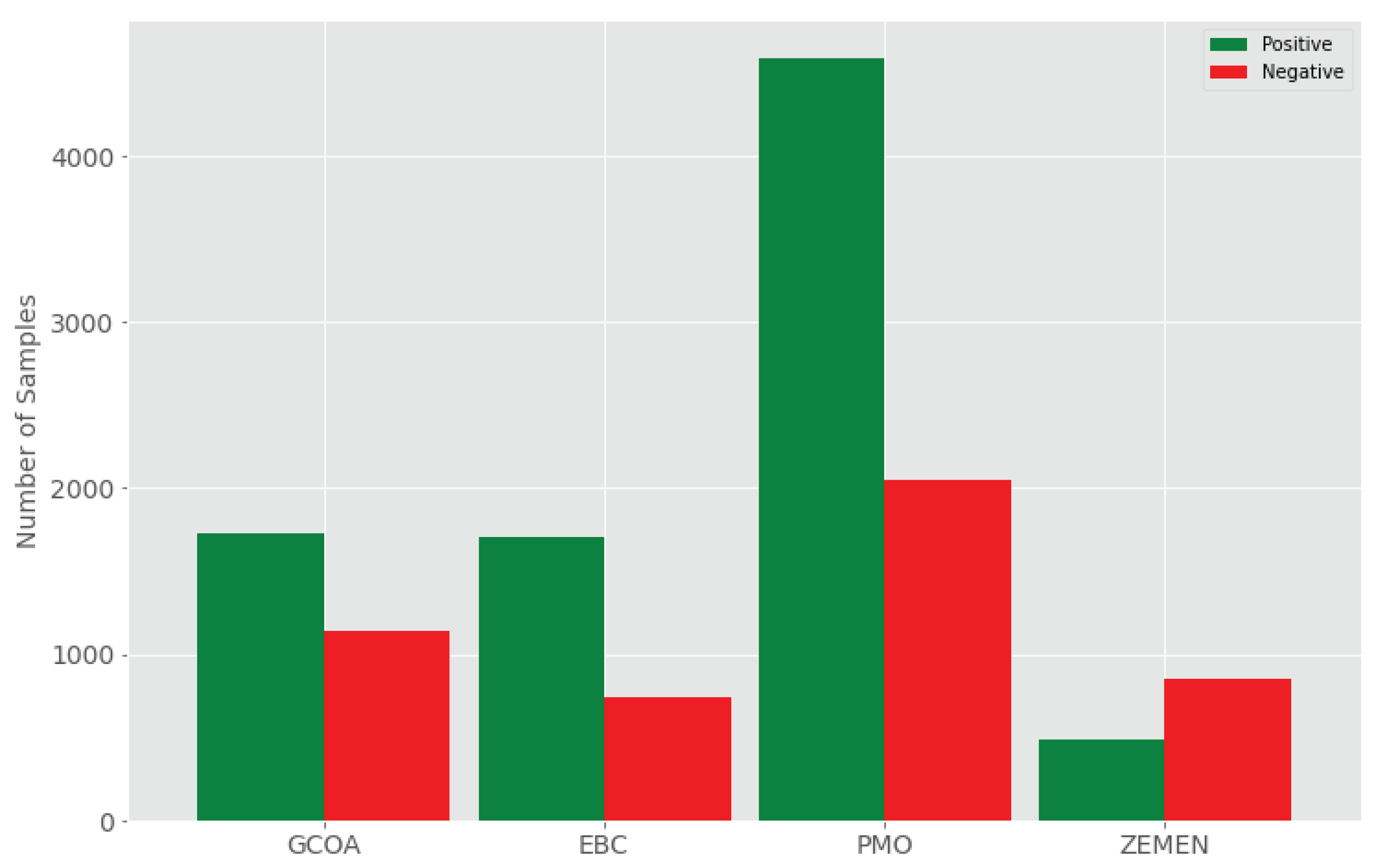
| Dataset | #Texts | Avg.chars | Avg.words | #Samples | #POS | #NEG | Year |
|---|---|---|---|---|---|---|---|
| GCOA | 2871 | 41.31 | 8.34 | 2871 | 1728 | 1143 | 2016–2017 |
| EBC | 2444 | 99.75 | 20.41 | 2444 | 1707 | 737 | 2017 |
| PMO | 6637 | 192.03 | 39.03 | 6637 | 4589 | 2048 | 2018 |
| ZEMEN | 1440 | 63.21 | 13.42 | 1440 | 490 | 850 | 2016–2018 |
| Algorithm | Hyper-Parameter | Type | Default Value | Selected Value |
|---|---|---|---|---|
| TF-IDFVectorizer | analyzer | discr | word | Char |
| max_df | cont | 1 | None | |
| max_features | discr | None | 5000 | |
| ngram_range | disc | (1,1) | (1,7) | |
| LR | C | cont | 1 | 1 |
| alpha | cont | None | None | |
| average | discr | None | None | |
| penalty | disc | l2 | l2 | |
| power_t | cont | None | None | |
| tol | cont | 0.0001 | 0.0001 | |
| Multinominal NB | alpha | con | 1 | 1 |
| NB | fit prior | cat | TRUE | TRUE |
| SVM | C | con | 1 | 1 |
| coef0 | con | 0 | 0 | |
| degree | discr | 3 | 3 | |
| gamma | con | scale | scale | |
| kernel | disct | rbf | rbf | |
| tol | con | 0.001 | 0.001 | |
| Random Forest | bootstrap | discr | TRUE | TRUE |
| criterion | disc | gini | gini | |
| max features | con | auto | auto | |
| min samples split | disc | 2 | 2 | |
| min samples leaf | discr | 1 | 1 | |
| n_estimators | discr | 100 | 100 |
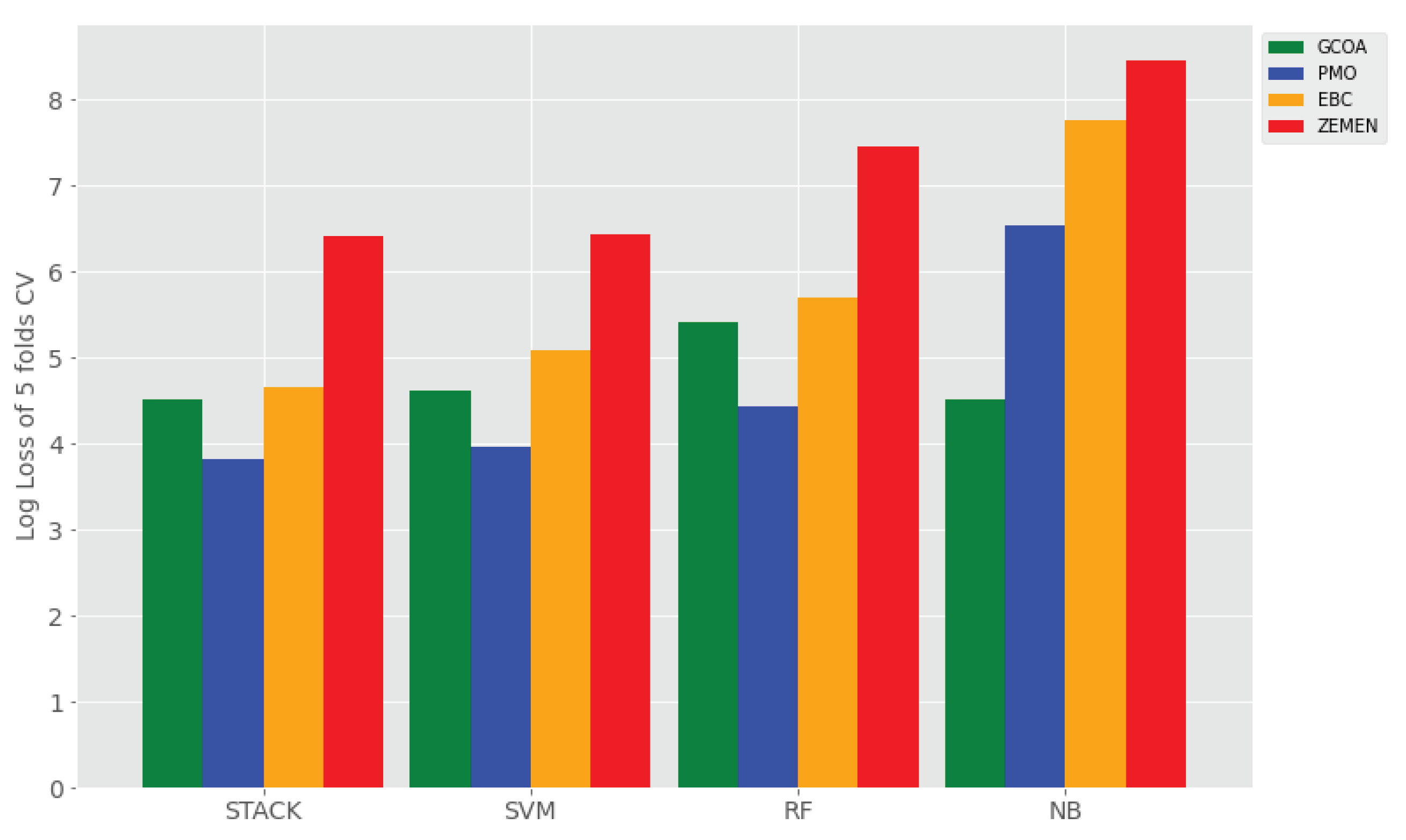
| Model | Metric | Exp I: CoS | Exp II: CS | Exp III: WoS | Exp IV: WS |
|---|---|---|---|---|---|
| Mean ± SD | Mean ± SD | Mean ± SD | Mean ± SD | ||
| SVM | Accuracy | 0.78 ± 0.02 | 0.85± 0.07 | 0.72 ± 0.01 | 0.74 ± 0.02 |
| Recall | 0.70 ± 0.02 | 0.85 ± 0.07 | 0.64 ± 0.01 | 0.74 ± 0.02 | |
| Precision | 0.79 ± 0.03 | 0.87± 0.06 | 0.70 ± 0.02 | 0.75 ± 0.03 | |
| F1 | 0.71 ± 0.02 | 0.85 ± 0.07 | 0.64 ± 0.02 | 0.73 ± 0.02 | |
| AUC | 0.84 ± 0.02 | 0.94± 0.04 | 0.72 ± 0.03 | 0.78 ± 0.04 | |
| LogLoss | - | 5.02 ± 2.38 | 9.63 ± 0.46 | 9.11 ± 0.85 | |
| RF | Accuracy | 0.76 ± 0.02 | 0.83 ± 0.07 | 0.72 ± 0.02 | 0.73 ± 0.03 |
| Recall | 0.69 ± 0.02 | 0.83 ± 0.07 | 0.65 ± 0.02 | 0.73 ± 0.03 | |
| Precision | 0.76 ± 0.03 | 0.84 ± 0.06 | 0.69 ± 0.02 | 0.75 ± 0.04 | |
| F1 | 0.70 ± 0.03 | 0.83 ± 0.07 | 0.65 ± 0.02 | 0.73 ± 0.03 | |
| AUC | 0.81 ± 0.02 | 0.92 ± 0.06 | 0.74 ± 0.02 | 0.81 ± 0.04 | |
| LogLoss | - | 5.77 ± 2.33 | 9.81 ± 0.53 | 9.18 ± 1.16 | |
| NB | Accuracy | 0.76 ± 0.02 | 0.79 ± 0.03 | 0.72 ± 0.02 | 0.68 ± 0.02 |
| Recall | 0.69 ± 0.02 | 0.79 ± 0.03 | 0.64 ± 0.02 | 0.68 ± 0.02 | |
| Precision | 0.76 ± 0.02 | 0.79 ± 0.03 | 0.72 ± 0.03 | 0.69 ± 0.02 | |
| F1 | 0.70 ± 0.02 | 0.79 ± 0.03 | 0.64 ± 0.02 | 0.68 ± 0.02 | |
| AUC | 0.82 ± 0.02 | 0.87 ± 0.03 | 0.75 ± 0.02 | 0.77 ± 0.02 | |
| LogLoss | - | 7.35 ± 1.18 | 9.51 ± 0.52 | 11.06 ± 0.82 | |
| Stack | Accuracy | 0.79 ± 0.02 | 0.86± 0.06 | 0.73 ± 0.01 | 0.74 ± 0.03 |
| Recall | 0.74 ± 0.02 | 0.86 ± 0.06 | 0.64 ± 0.01 | 0.74 ± 0.03 | |
| Precision | 0.77 ± 0.02 | 0.87± 0.05 | 0.71 ± 0.03 | 0.75 ± 0.04 | |
| F1 | 0.75 ± 0.02 | 0.86 ± 0.06 | 0.64 ± 0.02 | 0.73 ± 0.03 | |
| AUC | 0.84 ± 0.02 | 0.94± 0.04 | 0.76 ± 0.02 | 0.82 ± 0.03 | |
| LogLoss | - | 4.85± 1.95 | 9.49 ± 0.45 | 9.13 ± 1.11 |
Publisher’s Note: MDPI stays neutral with regard to jurisdictional claims in published maps and institutional affiliations. |
© 2021 by the authors. Licensee MDPI, Basel, Switzerland. This article is an open access article distributed under the terms and conditions of the Creative Commons Attribution (CC BY) license (https://creativecommons.org/licenses/by/4.0/).
Share and Cite
Neshir, G.; Rauber, A.; Atnafu, S. Meta-Learner for Amharic Sentiment Classification. Appl. Sci. 2021, 11, 8489. https://doi.org/10.3390/app11188489
Neshir G, Rauber A, Atnafu S. Meta-Learner for Amharic Sentiment Classification. Applied Sciences. 2021; 11(18):8489. https://doi.org/10.3390/app11188489
Chicago/Turabian StyleNeshir, Girma, Andreas Rauber, and Solomon Atnafu. 2021. "Meta-Learner for Amharic Sentiment Classification" Applied Sciences 11, no. 18: 8489. https://doi.org/10.3390/app11188489
APA StyleNeshir, G., Rauber, A., & Atnafu, S. (2021). Meta-Learner for Amharic Sentiment Classification. Applied Sciences, 11(18), 8489. https://doi.org/10.3390/app11188489