Article

Equal Baseline Camera Array—Calibration, Testbed and Applications

1
Faculty of Electronics, Telecommunications and Informatics, Gdansk University of Technology, ul. G. Narutowicza 11/12, 80-233 Gdansk, Poland
2
Center for Vision, Automation and Control, AIT Austrian Institute of Technology GmbH, Giefinggasse 4, 1210 Vienna, Austria
*
Author to whom correspondence should be addressed.
Appl. Sci. 2021, 11(18), 8464; https://doi.org/10.3390/app11188464
Submission received: 10 August 2021 / Revised: 2 September 2021 / Accepted: 8 September 2021 / Published: 12 September 2021
(This article belongs to the Special Issue Automation Control and Robotics in Human-Machine Cooperation)

Abstract

:
This paper presents research on 3D scanning by taking advantage of a camera array consisting of up to five adjacent cameras. Such an array makes it possible to make a disparity map with a higher precision than a stereo camera, however it preserves the advantages of a stereo camera such as a possibility to operate in wide range of distances and in highly illuminated areas. In an outdoor environment, the array is a competitive alternative to other 3D imaging equipment such as Structured-light 3D scanners or Light Detection and Ranging (LIDAR). The considered kinds of arrays are called Equal Baseline Camera Array (EBCA). This paper presents a novel approach to calibrating the array based on the use of self-calibration methods. This paper also introduces a testbed which makes it possible to develop new algorithms for obtaining 3D data from images taken by the array. The testbed was released under open-source. Moreover, this paper shows new results of using these arrays with different stereo matching algorithms including an algorithm based on a convolutional neural network and deep learning technology.

1. Introduction

This paper presents research on a camera array which consists of a central camera and up to four side cameras equally distant from a central one. Such an array has a function of a 3D vision system. The array was called Equal Baseline Camera Array (EBCA). It is derived from a stereo camera [1,2].
In general, researchers improve the quality of 3D data obtained from a stereo camera by designing more precise algorithms for processing pairs of images. The research presented in this paper is focused on improving 3D vision by taking advantage of a greater number of cameras. EBCA preserves benefits of a stereo camera while it provides a higher quality of data. The comparison of the considered array with other 3D imaging techniques such as structured light 3D scanning is presented in Section 2.1.
The main application of the research presented in this paper is the development of 3D vision systems for autonomous robots operating in outdoor environments. The research is derived from agricultural applications in which 3D vision sensors were applied to robotic fruit harvesting [2,3,4,5]. However, the array described in this paper can also be used with other kinds of autonomous machines including self-driving cars or unmanned underwater vehicles (UUVs). Section 7 lists applications in which the array can be used.
The paper also presents a method for calibrating cameras in the array including its intrinsic and extrinsic parameters [6,7,8]. We propose a hybrid method combining self-calibration techniques with a calibration based on taking images of a predefined patterns. The method is adjusted to distinctive features of the array as presented in Section 2.4, Section 4 and Section 6.
Another original contribution of this paper is the description of the testbed which was released for testing stereo matching algorithms intended to use with the considered array. The testbed was released under an open-source (https://github.com/alkaczma/ebca (accessed on 9 August 2021)). It is suitable for analyzing the improvement in the quality of results with regard to the number of side cameras in the array in the range between one and four. The testbed presented in this paper is inspired by well-known testbeds for evaluating stereo matching algorithms designed for obtaining disparity maps and depth maps using stereo cameras. The most popular this kind of testbeds are Middlebury Stereo Evaluation (http://vision.middlebury.edu/stereo/ (accessed on 9 August 2021)) [9,10] and KITTI Vision Benchmark (http://www.cvlibs.net/datasets/kitti/ (accessed on 9 August 2021)) [11]. In general, there is a lack of openly available testbeds for algorithms using camera arrays. This paper addresses this field of research. This topic is covered in Section 2.2 and Section 5.
Moreover, the paper describes the usage of Exception Excluding Merging Method (EEMM) with the proposed testbed [3]. This method was designed for obtaining 3D data on the basis of images taken by EBCA. Experiments presented in the paper verify the effects of changing values of parameters which are used in the method. This paper also shows how the quality of results depends on the number of cameras included in the camera array when the EEMM method is used. Section 6 describes tests of the method with four stereo matching algorithms including the algorithm which takes advantage of convolutional neural network (CNN) [12].
The original research presented in this paper includes the following. (1) The design and experiments with the calibration method for EBCA. (2) The description of the testbed designed for testing 3D imaging algorithms using the array. (3) Experiments with the EEMM method considering the selection of its parameters and the influence of the number of cameras on the quality of results. (4) Results of using Equal Baseline Camera Array with a stereo matching algorithm based on convolutional neural network.

2. Related Work

There is a large variety of technologies designed for 3D scanning—a recent comparison can be found in [13] and locating objects in 3D space. However, an appropriately calibrated camera array has remarkable advantages in comparison to alternative methods for acquiring 3D data.

2.1. 3D Vision Technologies

A 3D data acquisition is possible with the use of the following technologies:
  • Structured-light 3D scanners scan a 3D shape by emitting precisely defined light patters such as stripes and recording distortions of light on objects [14].
  • Light Detection and Ranging (LIDAR) measures distances to a series of distant points by aiming a laser in different directions [15].
  • Time-of-flight cameras (TOF) operate on a similar principle as LIDAR however instead of redirecting a measuring laser the entire measurement of distances is performed using a single light beam [16].
  • Structure from motion and multi-view stereo technologies record a 3D shape of an object by analyzing numerous images taken from different points of view located around the object [17] or by moving the object in front of a camera [18].
  • Stereo cameras resemble 3D imaging with the use of a pair of eyes. Stereo cameras record relative differences between locations of objects in images taken from two constituent cameras. The extent of these disparities depends on distances between a stereo camera and objects located in the field of view. The closer the object is, the greater is the disparity [3].
  • Camera arrays operate on similar principles as stereo cameras, however it takes advantage of a greater number of cameras [19,20].
3D imaging technologies have different features. None of these methods is the most suitable one in all circumstances. This paper contributes to development of methods for acquiring 3D data on the basis of a set of images obtained from a camera array. As far as camera based systems are concerned there are applications in which this equipment is especially valuable. Main advantages of a camera array are the following.
  • It can be used in highly illuminated areas. It is not possible to use structured-light 3D scanners in intensive natural light because external light sources interfere with the measurement performed by this kind of a sensor.
  • An array provides dense data concerning distances to parts of objects visible in the 3D space. In contrast to LIDARs and TOF cameras which can provide only sparse depth maps.
  • The technology of camera arrays can be flexibly used for measuring both small and large distances depending on a size of used cameras and types of their lens. Such a functionality is very limited when other kinds of 3D imaging devices are used.
  • 3D imaging with the use of array does not require relocating the imaging device to different positions. It is necessary when the technology of structure from motion or multi-view stereo (MVS) is used.
  • An array is a compact device which can be inexpensive if low-cost cameras are used.
  • The weight of an array constructed from small-sized cameras is low, therefore it can be mounted on moving parts of an autonomous robot (e.g., robotic arms) without putting much load on servos or other mechanisms driving the robot.
These advantages apply to both arrays and stereo cameras. The major disadvantage of a stereo camera is such that the quality of its results is lower than the quality obtained from other 3D imaging devices. This problem is reduced if camera arrays is used, in particular the kind of an array described in this paper (Section 3).
Another disadvantage of camera-based systems is such that it is time-consuming to process images from cameras in order to retrieve 3D data. This problem is even more serious in the case of using an array, as the number of cameras is greater. However, taking into account a rising speed of computer devices a greater number of computations is a reasonable cost of improving the quality of 3D imaging. A disadvantage of an array in comparison to a stereo camera is also the price of a greater number of constituent cameras. However, as in case of greater computational requirements, it is not a significant cost of obtaining a higher quality of 3D data.

Camera Arrays

Wang et al. presented a study on camera arrays and their applications [21]. They described using arrays both for depth recovery and for other applications such panoramic imaging. Manta presented a survey on preparing 3D videos on the basis of multiple cameras [22]. The usage of camera arrays for providing 3D vision in robotic applications was discussed by Nalpantidis and Gasteratos [23]. Camera arrays are widely used in astronomy for space observations. Ackermann et al. wrote a survey on this subject [24].
Wilburn et al. performed a study at Stanford University on constructing arrays from a large number of cameras. They built an array of 100 cameras in the 10 × 10 configuration and they applied it for making high quality images and videos [20]. Another significant camera array called PiCam was constructed by Venkataraman et al [25]. It was an ultra-thin array consisting of 16 cameras distributed uniformly over a square grid. The size of the array was similar to a size of a coin. The paper describing PiCam contains also an in-depth review on camera arrays usage. Okutomi and Kanade are the authors of a very influential research paper concerning arrays in which cameras are placed along a straight line [19]. Ge et al. proposed the usage of a sliding camera resembling a linear camera array [26].
A construction with a moving camera was also proposed by Xiao, Daneshpanah and Bahram Javidi [27]. They constructed a synthetic aperture integral imaging (SAII) by using a camera moving in two dimensions, making it possible to acquire images as if a camera array was used. Such a technique cannot be used for even slowly moving objects because the scene would be changing while subsequent images are taken. Authors applied their method for detecting and removing occlusions of objects in images.
Arrays containing only a few cameras are also constructed and used. Such arrays can be used for 3D imaging instead of stereo cameras without a substantial increase in the size of data which need to be processed due to the increase in the number of images. Park and Inoue proposed the usage of a five-camera array [1]. The array contained a central camera and side cameras. This kind of an array is also considered in this paper, and it is further described in Section 3. Hensler described a similar kind of an array which was constructed from four cameras with three side cameras placed on vertices of an isosceles triangle and a central camera located in the middle [28].
Ayache and Lustman wrote in 1991 a highly influential paper regarding trinocular vision [29]. They used the array for identifying contours visible in images and building a three-dimensional description of the environment. The performance of trinocular vision systems were also researched by Mulligan, Isler and Daniilidis [30,31]. Andersen et al. also used a trinocular stereo vision for navigating a robot [32]. Williamson and Thorpe applied trinocular vision to detect obstacles on highways [33].
Wang Xiao and Javidi performed research on using an array with unknown poses of cameras placed on a flexible surface [34]. The major advantage of this solution is the ease of construction. However, in case of such an array, there is also a necessity to identify locations of cameras. This process is performed on the basis of images for which a disparity map is obtained. When an array with predefined poses of cameras is used, then the step of resolving cameras locations is completed before using the array in the target environment. It speeds up the process of acquiring 3D data. Moreover, predefining locations makes it possible to place cameras in the most advantageous positions providing the highest quality of data.

2.2. Testbeds

Testbeds for testing 3D vision algorithms used with stereo cameras are widely used for improving the stereo vision technology. As mentioned in the introduction, Middlebury Stereo Evaluation is one of the most important sources of data for testing stereo vision algorithms [10,35]. As of 6 August 2021, there are in total 71 datasets in the testbed. Each dataset consists of a pair of images and ground truth reflecting real values of disparities for all objects visible in images. The testbed was prepared by Middlebury College and Microsoft Research in cooperation with US National Science Foundation. Apart from test datasets, the project releases a ranking of stereo matching algorithms. The current, third version of the ranking evaluates over 100 algorithms.
KITTI Vision Benchmark Suite is another evaluation system for stereo matching algorithms [36]. Datasets included in the benchmark consist of images taken from a stereo camera mounted on a car moving along streets. The testbed is foremost intended for selecting algorithms which are the most suitable for obtaining 3D data in autonomous cars. KITTI presents also a ranking of stereo matching algorithms. As of 6 August 2021, the ranking considers 316 algorithms.
There is also a test data set called NYU Depth Dataset V2 (https://cs.nyu.edu/silberman/datasets/nyu_depth_v2.html (accessed on 9 August 2021)) [37]. The set contains images of indoor sites. Apart from testing the quality of depth estimation results the set was prepared for evaluating image segmentation algorithms.
Moreover, the evaluation of stereo matching algorithms is possible with the use of ETH3D Benchmark (https://www.eth3d.net/ (accessed on 9 August 2021)) [38]. The benchmark provides image pairs taken in different sites including indoor and outdoor areas. The benchmark also presents the ranking of matching methods.
As far as test datasets for camera arrays are concerned, this kind of resources is only provided by the ETH3D Benchmark in a form of videos made with the use of a camera array consisting of 4 cameras placed along a line (https://www.eth3d.net/ (accessed on 9 August 2021)) [38]. The rig was constructed from two stereo cameras placed side by side. Authors of ETH3D used the rig to prepare 10 videos of different locations. A sample set of four images taken with the use of the rig is presented in Figure 1. ETH3D is the only testbed currently available for testing algorithms taking advantage of camera arrays.
There are also benchmarks for testing algorithms which obtain 3D scans from either a video recorded by moving camera or a set of images taken by a single camera from different points of view (multi-view stereo). Developing algorithms for these and other kinds of image processing is a subject of Robust Vision Challenge (http://www.robustvision.net/ (accessed on 9 August 2021)). The challenge is supported by leading companies such as Intel, Google, Apple, Bosch and Daimler. However, neither the challenge nor other sources of data for 3D vision make it possible to perform tests with camera arrays presented in this paper.

2.3. Stereo Matching Algorithms

Tests presented in this paper considered four stereo matching algorithms considered in Middlebury and KITTI rankings. These are the following algorithms: Efficient Large-scale Stereo Matching (ELAS) [39], Stereo Semi-Global Block Matching (StereoSGBM) [40,41], Graph Cut with Expansion Moves [42] and MC-CNN [12]. Open-source implementations of these algorithms were used in the experiments.
ELAS was designed for real-time processing of high-resolution images from stereo cameras [39]. The algorithm is intended for use with autonomous cars. StereoSGBM is the main algorithm provided with the OpenCV library which is one of the most important programming libraries in the field of image processing [41]. The GC Expansion algorithm was also included in experiments because the previous research on EBCA showed that adapting this algorithm to EBCA results in obtaining the best quality of disparity maps. The implementation of GC Expansion is provided by the Middlebury Stereo Evaluation project [9]. GC Expansion is a kind of a stereo matching algorithm which takes advantage of global optimization using Markov Random Fields (MRF) [43].
There are also stereo matching algorithms derived from deep learning technology which proved to be successful in solving a variety of algorithmic problems [44]. Zbontar and LeCun prepared an influential paper describing their stereo matching algorithm called MC-CNN which takes advantage of convolutional neural networks (CNN) [12]. They trained the network using stereo images and ground truth provided by the Middlebury Stereo Vision project and the KITTI benchmark. These authors used two kinds of network architecture. There was a fast network particularly dedicated for obtaining results in real-time and an accurate network focused on maximizing the quality of results. Each of these networks was trained with three different input data sets. These were training data sets from images released in the KITTI benchmark in 2012, another set was based on images from the KITTI set released in 2015 and the third data set was based on images available in Middlebury project. As a result Zbontar and LeCun obtained six trained networks marked as: KITTI 2012 fast, KITTI 2012 accurate, KITTI 2015 fast, KITTI 2015 accurate, Middlebury fast and Middlebury accurate. Moreover, their algorithm was released under open-source license making it possible for other researchers to rerun their experiments.

2.4. Calibration Methods

Camera calibration is the process of estimating the parameters of pinhole camera model, which ideally represents a camera taking an image. Here, one distinguishes intrinsic and extrinsic camera parameters [6]; for multi-view imaging, bundle adjustment [7,45] is applied for an image rectification.

2.4.1. The Math behind openCV’s Calibration

The notation complies with the camera model introduced in OpenCV Toolbox [41] and builds on the openCV toolbox. The intrinsic camera model has 9 degrees of freedom: two focal lengths f x , f y ; two principal point coordinates c x , c y ; three radial distortion parameters k 1 , k 2 , k 3 ; and two tangential distortion coefficients p 1 , p 2 , which comprise the distortion parameters d = ( k 1 , k 2 , p 1 , p 2 , k 3 ) . This vector d encodes the influence of the camera lens. The most evident this kind of a distortion is such that straight edges of real objects are depicted as bows in images. It is particularly visible when wide angle lens are used. These non-linear parameters are part of the geometric calibration, but will not be discussed further here, cf. [41]
The basic calibration transformation is presented as
s x y w p = f x 0 c x 0 f y c y 0 0 1 A r 11 r 12 r 13 t x r 21 r 22 r 23 t y r 31 r 32 r 33 t z [ R | t ] X w Y w Z w 1
where A is the intrinsic matrix encoding 4 of the 9 intrinsic parameters, and R and t are rotation and translation matrix, respectively. There are 6 degrees of freedom for extrinsic camera parameters [ R | t ] , which comprise position and rotation of the camera in a global coordinate system. NB, this matrix has 12 entries, but only 6 d.o.f., as the parameters r i j denote a rotation. s is a scaling factor. This form can be abbreviated as
s p = A [ R | t ] P w
It transforms every uncalibrated point P w to new coordinates p in a calibrated image with reduced distortions. The modification of this equation for the purpose of calibrating EBCA is presented in Section 4.1. In practice, one takes a pattern—openCV works with different types, but the most common is a checkerboard pattern that needs to be fully visible to the camera and presents it under different angles to the camera. openCV routines are used to extract the points of the pattern (say, the corners of the checkerboard). Furthermore, the user needs to input the dimensions of the checkerboard array (e.g., 6 by 8) and the distances between corners in some unit (e.g., mm) to the calibration algorithms, which outputs matrix A and for each image the calibration pattern the rotation R and translation t. This information (together with the computed distortion parameters d) allow for undistorting the images acquired by this camera into rectified views.

2.4.2. AIT Pattern vs. openCV’s Checkerboard

As a first step in every calibration method, a calibration target is presented in front of a camera and images of this target are acquired with every camera.
In order to facilitate better quality calibration with fewer acquisitions of the calibration target, the authors of [46] have developed a new central marker consisting of three asymmetric dots printed on an off-the-shelf high precision regular dot pattern calibration target (see Figure 2).
The main advantage of a calibration target with such a central element is that its markers may fill the entire field of view of the camera as long as the central element is readable. Moreover, this central marker is designed to be robust and easy to recognize while providing information about image mirroring.
In contrast, a typical checkerboard pattern is reflection symmetric, thus no information about mirroring is available. Furthermore, the openCV algorithm requires that the whole pattern is visible and that the user enters the dimensions of the board. In case of several cameras looking at the same scene such as the EBCA, it is particularly useful to have a pattern where only parts of the pattern need to be visible.
AIT’s pattern (see Figure 2) can been used in different sizes and for different resolutions. The central element (the three blue dots in Figure 2) should always be visible as well as one surrounding row of black dots, making 5 by 6 dots (as shown in the illustration) the smallest configuration for a stable detection. As a minimum requirement, the smaller dots should be resolved such that their diameter is at least 25 pixels wide, therefore the maximum number of black dots is only limited by the camera’s number of pixels. The distance between two dots should be at least a single dot’s diameter to allow for a stable distinction between neighboring dots.

2.4.3. Other Patterns

Other calibrating patterns have also been developed. Tao et al. proposed a pattern based on phase-shifting wedge grating (PWG) arrays which resembled annuluses in grayscale with varying light intensity [47]. They developed a feature detection algorithm for identifying centers of annuluses. They also applied a liquid crystal display for showing the pattern instead of a printed board.

2.4.4. Multi-Camera Calibration

Algorithms for performing calibration on a set of many cameras were proposed by Kang and Ho [48], Yang et al. [49] and Sun [50]. As far as calibration of stereo cameras is concerned there is a commonly used technique available in the OpenCV library [41]. OpenCV provides a calibration based on the Hartley’s rectification method [51]. This method was also adapted by authors of this paper for performing calibration on the EBCA array.
As opposed to pairwise stereo calibration like the standard openCV method, which usually requires one central camera to which all other cameras are calibrated; the work in [8] showed a multi-camera array calibration pipeline that fulfills all associated requirements.
The bundle adjustment [7] is a nonlinear method for refining extrinsic and intrinsic camera parameters, as well as the structure of the scene. For a set of n cameras with index i, it is characterized by minimizing the reprojection error by a standard least-squares approach
E ( C , P ) = i = 1 n w d i s t ( p i w , C i ( P w ) ) ) 2 ,
where C i ( P w ) = C ( A i , T i , d i , P w ) is the reprojected point as defined in Equation (2), i.e., the image of a point P w as observed by the i-th camera, which depends on the intrinsic matrix A i , the camera pose T i and the distortion parameters d i . Furthermore, p i w is the corresponding detected point of the calibration pattern and d i s t ( p i w , C i ) is the point’s reprojection error. For the details on this approach, please refer to the work in [8], where it is shown that the minimization of Equation (3) yields better reprojection errors and thus a higher 3D reconstruction quality than standard pairwise stereo approaches.
Bundle adjustment is designed for retrieving camera poses for the purpose of processing images with the use of multi-view stereo or structure from motion methods described in Section 2.1 [7]. Similarly as in camera calibration and rectification methods, in bundle adjustment points representing the same parts of objects are identified on different images. The identification of corresponding points is based on descriptors such as SIFT.
However, bundle adjustment has a different application than stereo camera calibration and rectification, because bundle adjustment is foremost performed to identify in a common 3D space camera poses from which images were taken. It is used when images are taken from different points of view located around viewed object and there is no need to make cameras parallel to each other. In the MVS technology, there is also a problem of taking images from proper positions. Hosseininaveh et al. addressed this issue in a case in which the number of images taken for the purpose of processing them using MVS is redundant [52]. They proposed a method for selecting suitable images.
Bundle adjustment generates some error in estimating camera poses in 3D space. This error needs to be considered in relation to distances between cameras. The impact of the error is not critical when cameras are not adjacent to each other. However, in case of using adjacent cameras such as those in a stereo camera it is crucial to perform calibration with higher precision using predefined patterns such as chessboards.
Stereo camera and camera array calibration is dedicated not only to a case when cameras are located close to each other, but also they are aimed at the same direction and there is a selected reference camera which is a point of view of the entire set. The purpose of stereo camera calibration and rectification is to transform 2D images in order to reduce as closely as possible any differences from the ideal case in which camera are parallel to each other without any inaccuracy. Stereo cameras and camera arrays has a function of depth camera. Such devices are used when it is hard or even impossible to take images from around an object in order to retrieve its 3D structure. Stereo camera calibration converts 2D images so that they are sufficient for processing with the use of stereo matching algorithms. Bundle adjustment operates directly on 3D space. Disparity maps obtained from stereo matching algorithms can be converted to distances between a reference camera and objects visible in images [19]. The quality of a resulting depth map depends on the quality of obtained disparity maps.

2.5. Self-Calibration

Another approach to reducing distortions in images is based on self-calibration also called autocalibration. Self-calibration results in rectifying images without the use of any predefined, exemplary pattern. Images are transformed only on the basis of their content. Self-calibration is performed in stereo cameras mainly to reduce extrinsic distortions caused by the fact that side camera is aimed at slightly different direction than a reference one and side camera may be rotated with respect to a reference one.
Algorithms for performing self-calibration are based on features extraction and finding the same keypoints in both images. One of the most well-known algorithms for identifying keypoints is Scale-invariant feature transform (SIFT) [53]. This algorithm was used for self-calibrating stereo cameras by Liu et al. [54]. SIFT was a base for developing commonly used Speeded up robust features (SURF) algorithm [55]. However, other methods for identifying keypoints are also used for performing self-calibration of stereo cameras. Boukamcha, Atr andSmach compared seven techniques for features extraction: SIFT, SURF, BRISK, FAST, FREAK, MinEigen and MSERF [56].
A vast amount of research regarding calibration and autocalibration is focused on calibrating stereo cameras and camera rigs for the purpose of using them with autonomous cars. Mentzer et al. applied for this purpose A-KAZE-feature extraction [57]. Carrera, Angeli and Davison used feature SURT extraction technique for calibrating multi-camera rig [58]. Heng et al. applied a similar approach for the rig mounted on a car [59].

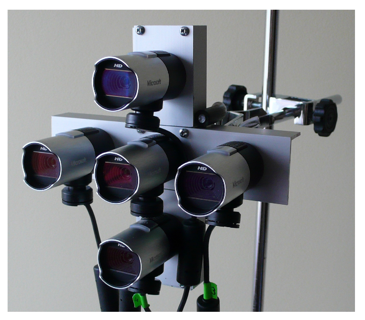
3. Equal Baseline Camera Array

The array described in this paper is called Equal Baseline Camera Array (EBCA) [1,2]. In previous papers the author of this paper called it Equal Baseline Multiple Camera Set (EBMCS), however the name was changed because the current one is more adequate [3,4,5]. A real camera set mounted in the form of Equal Baseline Camera Array (EBCA) is presented in Figure 3. The figure presents the set consisting of MS LifeCam Studio cameras with the 1080p HD sensor.
Park and Inoue were the first to research the possibilities of using a camera set arranged in the form of Equal Baseline Camera Array with five cameras [1]. Research concerning such a set was also conducted by Fehrman and McGough who were in possession of a larger camera array but they selected from their array a five camera subset [60,61]. The author of this paper is further developing this technology [2,3,4,5,62].
EBCA consists of up to five cameras placed in such a way that there is a central camera and up to four side cameras. The distance between every side camera and a central camera is the same. Such a distance is called a baseline. In real devices there are some inaccuracies causing that baselines are not equal to each other. However, distortions occurring in images caused by these imperfections are corrected in the calibration process. Side cameras are placed on opposite sides of a central camera in vertical and horizontal dimensions.
The set with five cameras has a function of combined four stereo cameras created by a central camera paired with different side cameras. These stereo cameras will be marked with C 1 (right pair), C 2 (up pair), C 3 (left pair), and C 4 (down pair).
The central camera is a reference one in each considered pair of cameras. Algorithms processing images from stereo cameras distinguish between a reference camera or a side one. A reference camera is a point of view of a stereo camera. Side cameras are used to acquire disparity maps for points visible from the reference camera.
In EBCA, every considered stereo camera shares the same reference camera which is the central camera in the set. It is an important benefit of this kind of a camera set because 3D data acquired from each constituent stereo cameras can be easily merged together in order to acquire data which is more precise than those based on a single stereo camera.
EBCA resembles a linear camera array. However, in general, pairs of cameras which can be selected from a linear stereo array may have a different reference camera or differ in sides of baselines. The problem with inequality of baselines is such that it influences the disparity. The increase in the size of a baseline cause that disparities became greater. It is more problematic to merge data from stereo cameras with different baselines. Okutomi and Kanade addressed this problem which is particularly significant in leaner camera arrays [19]. Moreover, stereo cameras selected from a leaner camera array may have different reference cameras. The problem with merging data from such stereo cameras is also complicated because of the necessity to unify points of view of camera pairs. This problem does not occur when EBCA is used.

3.1. Exceptions Excluding Merging Method

This paper presents also results of new research on modifying parameters used in Exceptions Excluding Merging Method and applying the method to arrays with different number of cameras. The EEMM method was designed by the author of this paper with the purpose of improving the quality of disparity maps by taking advantage of EBCA instead of using a single stereo camera. The research presented in [2,3] shows that the method fulfills its requirements.
EEMM is based on eliminating values of disparities which deviate from other values provided by stereo cameras included in EBCA. Every point of a disparity map represents either a value of a disparity or a value indicating that the disparity is unknown. There are stereo matching algorithms which obtain disparities for all points of a map. There are also algorithms which provide information that it was not possible to determine disparities in some points. Therefore, when N disparity maps are merged, then the number of disparities used for calculating each resulting disparity is in the range between zero and N. EEMM differently calculates disparities depending on the number of constituent values.
Details of the algorithm are described in [3]. The results of the method depends on two parameters Q and B which are considered in the experiments presented in this paper. In case of having two disparity maps with a value in point, results of the EEMM method depends on a parameter Q. The existence of three disparities in merged disparity maps cause that the parameter B is used. The original version of EEMM required that B = Q / 2 .
The previous version of the algorithm presented in [3] was designed for an array of exactly 5 cameras, i.e., one central camera and four side cameras. In this paper we propose a version of this algorithm for arrays consisting of only two or three side cameras. For some applications, it could be advisable to use less than five cameras and the aim of this research is to show the extent of improvement with respect to the number of used cameras.
Another original results covered by this paper is the problem of setting parameters Q and B. This paper show results of a generalized version of the algorithm in which B Q / 2 i.e., parameters are set independently from each other. In some applications it can be necessary to set parameters in such a way that the error rate of disparity maps is lower in exchange for a greater size of areas in which disparity is undetermined. In other application it may by crucial to keep the area of undetermined disparities are low as possible. It can be controlled with the use of parameters Q and B.

4. Calibration of the Camera Array

Methods of calibrating and rectifying images described in Section 2.4 do not completely cover transformations which need to be performed in order to calibrate and rectify EBCA. Moreover, techniques based on bundle adjustment are also insufficient because they are designed for other kinds of camera locations as presented in Section 2.4, in which work performed by Hosseininaveh et al. is discussed [52]. In this paper, the stereo camera calibration methods described in Section 2.4 were used. However, in adapting existing stereo camera calibrating methods to EBCA there are two missing steps: The first problem is ensuring that all stereo cameras considered in EBCA will produce a disparity map referring to the same central image, because EBCA is designed to make it possible to easily merge data obtained from different camera pairs. The second problem is calibrating baselines. Solutions for both of these two issues are introduced in Section 4.1 and Section 4.2 of the paper.
A large majority of stereo matching algorithms and calibrating algorithm are designed and implemented with such an assumption that the algorithm will be used with a stereo camera consisting of a left camera and a right camera. Disparities occur in the X dimension. In fact, every stereo matching algorithm can be similarly implemented to process images which were taken by lower and upper camera. However, it requires modifying existing implementations of algorithms for stereo cameras. It is particularly problematic when an there is no open-source implementation. This paper proposes a method in which instead of re-implementing existing software the images are flipped and rotated in such a way that they can be perceived by stereo matching algorithms a pair consisting of a left, reference image and a right, side image. After these operations disparity maps refer to points of the same central image regardless of the side camera used in EBCA. Section 4.1 describe transformations required to achieve this.
The second problem is calibrating baselines in EBCA. It is beneficial for the quality of disparity maps obtained from EBCA when distances between cameras are as closely similar to each other as possible. However, in real devices inaccuracies occurs. In case of using stereo cameras such a problem does not exist because there is only one baseline in a stereo camera. Therefore, the problem of calibrating baselines appears when images from EBCA are processed. However, all previously performed research on camera arrays such as EBCA described in Section 2.4 did not cover methods of calibrating baselines. Therefore, this paper introduce a method described in Section 4.2.

4.1. Pairwise Calibration

A pairwise calibration and rectification presented in this section is based on OpenCV calibration algorithms implementing the calibration method proposed by Zhang and the rectification method introduced by Hartley [41,51,63]. In order to obtain calibrated of images taken by EBCA using OpenCV based method raw images (marked with I R ) need to be processed in few stages. This process in visualized by Figure 4. The first part of image processing is using calibration data for rectifying images in order to reduce distortions. This calibration is based on taking images of a predefined pattern as described in Section 2.4.
Raw images I R were processed as if they were taken by a set of four stereo cameras sharing a common camera which was the central one. I R 0 , I R 1 , I R 2 , I R 3 and I R 4 will denote raw images from a central, right, up, left and down camera, respectively. A sample set of raw images used in experiments is presented in Figure 5.
Results of the image calibration consist of four pairs of images. The entire set of these pairs is marked with I P . I C k will denote a reference image in pair k and I S k will be a side one in this pair. A sample set of pairs is presented in Figure 6.
Pairs I P are intended to be used as input data to stereo matching algorithms designed for processing images from stereo cameras. Every pair of images is derived from an image taken by a central camera and an image from one of side cameras. In EBCA locations of side cameras with regard to a reference, central camera is different. However, each considered pair of cameras is regarded as a stereo camera consisting of a left and right camera. Therefore, images were rotated and flipped in order to adapt them to such a configuration. Equation (2) used for calibrating pairs of cameras takes the form
s p = W k A [ R | t ] P w
where W k is a matrix converting every pair of a central image and a side one to a pair which can be perceived as two images taken from a reference camera and a side camera located on the right side of a reference camera. Index k corresponds to the position of a side camera in the camera array. The whole transformation W k A [ R | t ] will be marked with E k in this paper.
Transformation W k is the same for a central image and a side image within the same stereo pair. An image from a central camera has a function of a reference image in every pair of cameras considered in EBCA, therefore this image in transformed differently for the purpose of using it with different side images.
Figure 6 presents pairs of rectified strawberry images. Images were converted to grayscale as most of stereo matching algorithms process images in this form.
There are four cases:
right camera
The right camera forms with the central camera a standard stereo camera, therefore neither a rotation or an flipping is needed. Thus, in this case W 1 = I .
up camera
Images from a pair consisting of top and central camera were first rotated 90 counterclockwise and than flipped around y-axis. The matrix W 2 defining the transformation for the pair created with the use of up camera is equal to the value presented in Equation (5).
W 2 = 0 1 2 c y 1 0 2 c x 0 0 1
where ( c x , c y ) is the center of an image. This value needs to be considered because point (0,0) is not located in the middle of the image, but it is in top left corner of an image affecting transformation matrices. The matrix was also calculated with regard to the convention such that coordinates of points in an image rises in the Y dimension from the top to bottom unlike in the commonly used Cartesian coordinate system.
left camera
Images from a left camera with corresponding images from a central camera were flipped around y-axis. Therefore,
W 3 = 1 0 2 c x 0 1 0 0 0 1
bottom camera
In case of using a stereo camera consisting of a bottom camera and a central one images were rotated 90 counterclockwise.
W 4 = 0 1 0 1 0 2 c x 0 0 1
Stereo matching algorithms process pairs of images I P which were obtained by applying calibration transformations on images I R . Thus, points in a disparity map obtained as a result of using matching algorithms refer to points of a transformed central image as this image is regarded as a reference one in every considered pair of images. The central image is differently transformed in every considered image pair. In order to acquire disparity maps whose points correspond to points of a raw central image, it is necessary to perform transformations reversing in disparity maps the calibration process. These reverse transformations including flipping and rotating images described earlier.
Maps obtained after reverse transformations can be further processed. Further processing can result in merging maps obtained from individual image pairs in order to acquire a map which has a higher quality than constituent maps. This is a subject of EBCA merging methods described in [2,3]. If ground truth is available then results can be compared in order to estimate the quality of stereo matching.

4.2. Self-Calibrating Baselines

A typical stereo camera self-calibration is focused on retrieving extrinsic parameters of a camera pair. The aim is to calibrate cameras so that a point p r from the reference image is correctly matched with a point p s from a side image and as a result a correct disparity d is identified. In case of the EBCA array, there are more tasks. Lets consider points p s k from I C k , k 1 , 2 , 3 , 4 , corresponding to the same point p r 1 in raw image I R 0 . Points p s k needs to be correctly matched with points in every side image I S k . As a result, disparities d k are obtained. However, in case of EBCA, it is expected that d 1 = d 2 = d 3 = d 4 .
Even if correct values of d k are obtained for every considered camera pair these values may not be equal to each other, because inaccuracies in the construction of EBCA. Theoretically, baselines of all considered stereo cameras are the same, but in real devices there are always some minor differences in baseline lengths. Baselines of considered stereo cameras C k may differ to such an extent that there are differences of at least few pixels between values of d k . This deteriorates the quality of resulting disparity map because when data is merged from all four C k under the assumption that baselines of these cameras are the same. Nevertheless, due to the self-calibration process described in this section images can be rectified in order to reduce differences between disparities d k .
The rectifying transformation defined in the self-calibrating process will be denoted by M k , where k corresponds to a camera pair C k . Let us first consider merging disparities for a single point p r 1 . Let us assume that a stereo matching algorithm correctly acquired disparities d k for this point. Thus, there are
d 1 = d ( p r 1 , I S 1 ) d 2 = d ( p r 1 , I S 2 ) d 3 = d ( p r 1 , I S 3 ) d 4 = d ( p r 1 , I S 4 )
where I S 1 is a side image after transformations as described in Section 4.1. We are willing to obtain disparities d 2 , d 3 and d 4 presented in Equation (9) such that d 1 = d 2 = d 3 = d 4 .
d 1 = d ( p r 1 , I S 1 ) d 2 = d ( p r 1 , M 2 I S 2 ) d 3 = d ( p r 1 , M 3 I S 3 ) d 4 = d ( p r 1 , M 4 I S 4 )
Values of d will be equal to each other if transformations M k cause that points of images I S k are shifted in the X dimension for numbers of pixels equal to m k such that, m k = d k d k for k 2 , 3 , 4 . For different points of image I S k desired values of m k may be different as there can be different values of d k d k for different points of I S k . Therefore, translation matrices M k needs to be obtained with regard to the entire image I R 0 .
This paper introduces estimating the shift m k of images I s k on the basis of keypoints acquired by the SURF algorithm [55]. Keypoints in the reference image and corresponding keypoints in side images are identified in image pairs I P obtained after transformations E k described in Section 4.1.
Let O k denote a set of matching keypoints in a pair consisting of a reference image I C k and side image I S k . For different k there will be different keypoints in images I C k and I S k . However, there will also be such keypoints o C k in images I C k which are derived from the same point o 0 of the raw image I R 0 transformed to different coordinates because of calibrating transformation E k . Such keypoints are those for which condition presented in Equation (10) is fulfilled.
o C k O k such that k { 1 , 2 , 3 , 4 } Q k ( o 0 ) = o C k
In this paper, only these keypoints o C k are considered in calculations of array rectification transformations M k . Thus, in every considered stereo camera, the set of the same points from a raw central image I R 0 is a base for analyzing differences in disparities provided by different cameras.
The subsequent step in calculating transformation M k with the use of the SURF algorithm is calculating disparities d o k between keypoints identified in images I C k and matching keypoints in images I S k . Those keypoints for which d o k is not within the range of disparities used for obtaining disparity maps by a stereo matching algorithm are excluded from further calculations. Excluding these values adjusts self-calibration to parameters of stereo matching algorithms. Thus, conditions d m i n d o k d m a x are fulfilled.
Then, an average value d o k , a v g of the the remaining disparities is calculated for each image pair I C k and I S k . The average value of disparities between matching keypoints indicates which pair of images should be rectified by M k so that disparities become larger and which pairs should provide lower values of disparities. Disparities for different image pairs are being adjusted to the pair I C 1 and I S 1 obtained from the central image and the right one taken by EBCA, so m 1 = 0 . Therefore, the extent of shifts m 2 , m 3 and m 4 that transformations M k should implement are given by Equation (11).
m 2 = d o 1 , a v g d o 2 , a v g m 3 = d o 1 , a v g d o 3 , a v g m 4 = d o 1 , a v g d o 4 , a v g
Thus, transformations M k are equal to the matrix presented in Equation (12).
M k = 1 0 m k 0 1 0 0 0 1
Equation (4) used for calibrating cameras in EBCA takes the following form:
s p = M k W k A [ R | t ] P w
Section 6.1 shows results of experiments with using transformations M k to improve the quality of disparity maps obtained from EBCA.

5. EBCA Testbed

This section describes a testbed which was released under an open-source license in order to make it possible for other researches to develop new and better algorithms using considered camera arrays. The application is available at (https://github.com/alkaczma/ebca accessed on 9 August 2021). The testbed was released as a part of work on this paper.
The testbed is suitable for evaluating a usage of all camera sets consisting of a central camera and up to four side cameras equally distant from a central one. In particular, algorithms designed for trinocular vision systems can be evaluated. The testbed can be used for both testing an array consisting of three cameras placed in a row and an L-shape trinocular vision system [29,31]. Moreover, test data presented in this paper include images necessary for testing arrays with four and five cameras. There are currently no openly available testbeds which makes this possible.
The testbed consists of six data sets and the software necessary for running experiments. Data sets used in the testbed contain images of plants. There are two data sets for every considered species including strawberries (sets marked with S T 1 and S T 2 ), redcurrants ( C U 1 and C U 2 ) and cherries ( C H 1 and C H 2 ). Every data set was created on the basis of five images taken by EBCA. Figure 5 presents a sample data set which is S T 1 containing images of a strawberry plant.
In the testbed calibration, the methods described in Section 2.4 and Section 4 were used. Calibration was based on taking images of an exemplary image pattern which was a chessboard with 10 × 7 intersections of black and white fields. Each field has a side equal to 24 mm. The set of images used for calibrating cameras consisted of 10 series of five chessboard images taken by EBCA from different angles. The OpenCV library was used for analyzing images and calculating transformations matrices used for refining images.
The process of preparing images for a testbed also consisted of cutting out parts of images taken by EBCA. Cameras made images with the resolution of 1280 × 720. The entire content of images was not used. Experiments were performed on parts of these images containing leaves and at least one fruit. In every data set, the selected parts of images were those which were located at the same coordinates in side images and a central one. The sizes of image parts which were used for making test sets are presented in Table 1.
The content of a central image can be distinguished between a matching area (MA) and a margin (MR). M A is a part of an image for which a disparity map is acquired. M R is the area placed around M A . M R contains auxiliary data used for calculating disparities in M A . Locations of objects in M A of the central image are shifted in side images with regard to positions of side cameras. Without a margin some objects located near borders of M A of a central image would not be visible from points of view of side cameras. Thus, both M A and M R need to be included in calculations in order to provide data for calculating disparities in M A .
The size of a margin needs to be greater than the maximum disparity that occurs in M A . After cutting out significant parts of raw images and calibrating them, the resulting images can be then processed by a stereo matching algorithm in order to retrieve a disparity map. Maximum disparities in different data sets are presented in the last column of Table 1. In all cases the maximum disparity is lower than 100. In previous experiments described in previous papers sizes of margins were not equal to each other [2,3]. Margins of images included in the testbed presented in this paper were unified and in every data set the margin covers all points located within the range of 100 points from borders of M A . The total number of test points existing in matching areas of all considered data sets is equal to 172,400.
The testbed contains also ground truth. Ground truth was prepared manually by identifying in images locations of points corresponding to the same parts of plants. Such an analysis is very time-consuming, however it allows acquiring correct values of disparities in points considered in experiments. The main problem with determining ground truth manually is the occurrence of monochrome areas such as walls for which it is impossible to find points corresponding in different images to the same parts of real objects. However, test data do not contain such surfaces as plants visible in images have non-uniform textures.
Ground truth data contain disparities referring to points of raw images I R 0 . However, stereo matching algorithms process pairs of images I P which were obtained by applying calibration transformations on images I R . Thus, points in a disparity map obtained as a result of using matching algorithms refer to points of a transformed central image as this image is regarded as a reference one in every considered pair of images. The central image is differently transformed in every considered image pair. In order to compare ground truth with disparity maps generated from different image pairs, it is necessary to perform transformations reversing in disparity maps the calibration process. Such transformations were also prepared by the author of this paper. Files ebmcscalibration.xml available in the testbed contain data necessary to reverse transformations including flipping and rotating images.
Maps obtained after reverse transformations can be either compared with ground truth or further processed. Further processing can result in merging maps obtained from individual image pairs in order to acquire a map which has a higher quality than constituent maps. Performing such a data merge is a subject of Exceptions Excluding Merging Method.

Evaluation Metrics

Disparity maps acquired by stereo matching algorithms can be evaluated with the use of different quality metrics [10,36]. Metrics used in the testbed and experiments presented in this paper are the following: the percentage of bad matching pixels (BMP), the percentage of bad matching pixels in background (BMB) and the coverage (COV) [2,3,10]. The formula for calculating BMP is presented in Equation (14).
B M P = 1 N p D M ( p ) D T ( p ) > Z
where p is a point, D M ( p ) is the disparity in the point p in the evaluated disparity map, D T ( p ) is the ground truth disparity, N is the total number of points and Z is the threshold considered in the metric. If the difference between the correct disparity and disparity indicated by the stereo matching algorithm does not exceed Z, then the estimation of the disparity is regarded as correct.
BMP presented in Equation (14) estimates the quality of disparities obtained for objects visible in the foreground. These objects are visible both in a central and side images, thus it is possible to estimate their disparities. Objects located in the background can be only partially visible in different images because from points of view of some cameras these objects can be hidden behind other objects located in the foreground. Therefore, it can be impossible to match patterns corresponding to the same object in different images. The estimation of the quality of disparities for objects located in the background is the subject of the BMP metric presented in Equation (15). The metric provides information on the percentage of points for which a stereo matching algorithm set incorrect values of disparities instead of indicating that disparities in these points are unknown.
B M B = 1 N B p D M ( p ) 0 D T ( p ) = 0
where N B is the number of points in background and other symbols are the same as in Equation (14). A value of a disparity equal to 0 means that the disparity is unknown.
Another considered metric is COV which corresponds to the percentage of points for which stereo matching algorithm was able to identify disparities. The formula for this metric in presented in Equation (16).
C O V = N L N
where N L is the number of points in a disparity map and N is the total number of considered points.

6. Experiments

This section presents results of self-calibration (Section 4.2), the influence of EEMM parameters on the quality of results (Section 6.2) and the influence of the number of cameras included in the array (Section 6.3).

6.1. Results of Self-Calibration

The self-calibrating method described in Section 4.2 was evaluated on the basis of comparing results obtained from images for which the method was applied with results obtained from images which were not processed by the method. Thus, two collections of image sets were prepared. The collection A contained images calibrated only with the pairwise method described in Section 4.1. The collection B were images acquired from the collection A after self-calibration. Collections A and B were prepared from the same images which were used for making test data in the testbed. All six sets of images were included in both of these collections.
Collections A and B had a function of input data used for acquiring disparity maps. First, considered pairs of images included in collection were processed by stereo matching algorithms. Then, results were merged using the EEMM method. Therefore, disparity maps were results of processing images from all five cameras included in the array. Algorithms considered in this experiments were ELAS, StereoSGBM and GC Expansion. Figure 7 shows results with regard to the collection used.
The first raw of charts in Figure 7 presents results for collection A (marked with Col A) and B (marked with (Col B). The lower raw visualize decreases in values of metrics obtained for collection B with regard to their values for collection A. Results of COV and BMO quality metrics are similar as they differ between collections less than 2.5%. However, the value of BMP is on average 34.2% lower than in case of using collection A. It is a significant improvement which shows that self-calibration method described in Section 4.2 is a valid technique of calibrating EBCA.
The required applied shifts were different for different data sets. On average the shift m 2 for the up camera was equal to 0.83, shift m 3 corresponding to the right camera was equal to 0.33 and m 4 for the down camera was 3.33. There were also differences in values of m for different data sets. However, the greatest deviation from the average values was lower than 5 points. For example, a 2 for set R C 1 was equal to −4, but for set R C 2 it was equal to 5. These values are high enough to influence the quality of resulting disparity maps, because they indicate that for the same points disparities calculated by different camera pairs differ between each other to this extent.
Differences in shifts for different data sets were foremost cause by different characteristics of these sets. As presented in Table 1 there are different ranges of disparities occurring in sets. Distances from which images were taken for different sets also varied. Moreover, sizes of sets were different. It is also presented in Table 1. Raw images I R were made with the resolution of 1280 × 720 however depending on the set parts of different sizes were cut out from raw images. Moreover, there are also variations caused by contents of images causing that SIFT matches different points depending on the analyzed set.

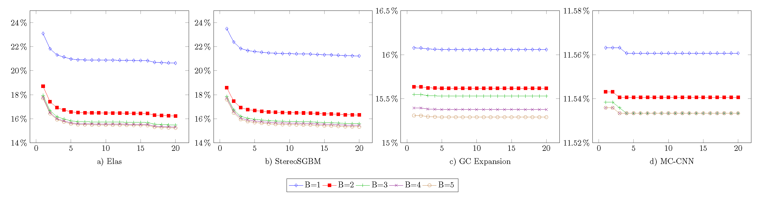
6.2. EEMM Parameters

The possibilities of selecting parameters B and Q in the EEMM method (Section 3.1) and their influence on the quality of disparity maps is presented in Figure 8, Figure 9 and Figure 10. Figure 8 shows values of the BMP metric when 1 B 5 and 1 Q 20 . The figure contains four parts showing results of using EEMM with four different stereo matching algorithms which are ELAS, StereoSGBM, GC Expansion and MC-CNN. The usage of MC-CNN was based on the KITTI 2015 accurate trained network provided by the author of the MC-CNN algorithm. Results presented in charts are average values obtained from all six data sets included in the testbed. Average values were calculated with respect to differences in sizes of matching areas presented in Table 1. The Y axes in Figure 8 refer to values of the BMP metric. The X axes correspond to values of the parameter Q. Each chart contains five lines which depict results for different values of B. The algorithm GC Expansion is influenced by random values and it generates different results for subsequent executions with the same input parameters. Therefore, results presented in figures for this matching method are average values calculated from ten executions of the algorithm.
Figure 8 shows that in case of all tested stereo matching algorithms the greater value of the parameter B results in lower values of the BMP metrics. It is an advantageous effect as low values of BMP indicate higher quality of maps. Experiments were also performed for greater values of B however the increase of this parameter did not cause significant the decrease of BMP. As far as the parameter Q is concerned, the increase of its value also causes the decrease of BMP. Note that for algorithms ELAS and StereoSGBM the improvement is the most significant in the range of B between 1 and 5. Greater values of B also cause that BMP become lower however this effect is not as significant as in case of B 5 . Such a characteristic does not occur with the GC algorithm in which there is a steady increase of the BMP values for the entire range of tested values of B. As far as MC-CNN algorithm is concerned, parameters B and Q affect values of BMP to an even lesser extent than in case of GC Expansion. Note that in the Y axis there is a range between 98.62% and 99.66% for GC Expansion and the range is only between 99.93% and 99.99% for MC-CNN.
Values of metrics BMB and COV were also acquired using the same input arguments as in case of the BMP metric. Results are presented in Figure 9 and Figure 10. A relation between parameters of EEMM and values of the COV metric is similar as in case of BMP. The increase in values of both B and Q results in obtaining more advantageous values of COV.
The improvement of the BMP value is, however, related to the increase of the BMB value. It is particularly problematic in case of using Q 5 with ELAS and StereoSGBM. When Q increases there is a much greater increase in the value of BMB than a decrease of the BMP value. Therefore, setting Q to 5 is an optimal solution. As far as the GC Expansion algorithm is concerned the increase of Q always causes the increase in BMB without a significant influence on the value of BMP. Thus, for this algorithm Q should be set to 1. Differences in results of BMB are the lowest in case of MC-CNN, however charts for this algorithm have characteristics similar to charts obtained for GC Expansion. Thus, Q equal to 1 is a recommended setting for MC-CNN with respect to results of BMB.
Figure 11 presents sample disparity maps obtained using a single stereo camera and EBCA. In the upper part of the figure there are four disparity maps retrieved on the basis of two cameras using algorithms ELAS, StereoSGBM, GC Expansion and MC-CNN, respectively [12,39,40,41,42]. The lower part of the figure contains disparity maps which were obtained when these algorithms were applied to EBCA with the use of EEMM. Parameters B and Q used in Exceptions Excluding Merging Method were set to 5.

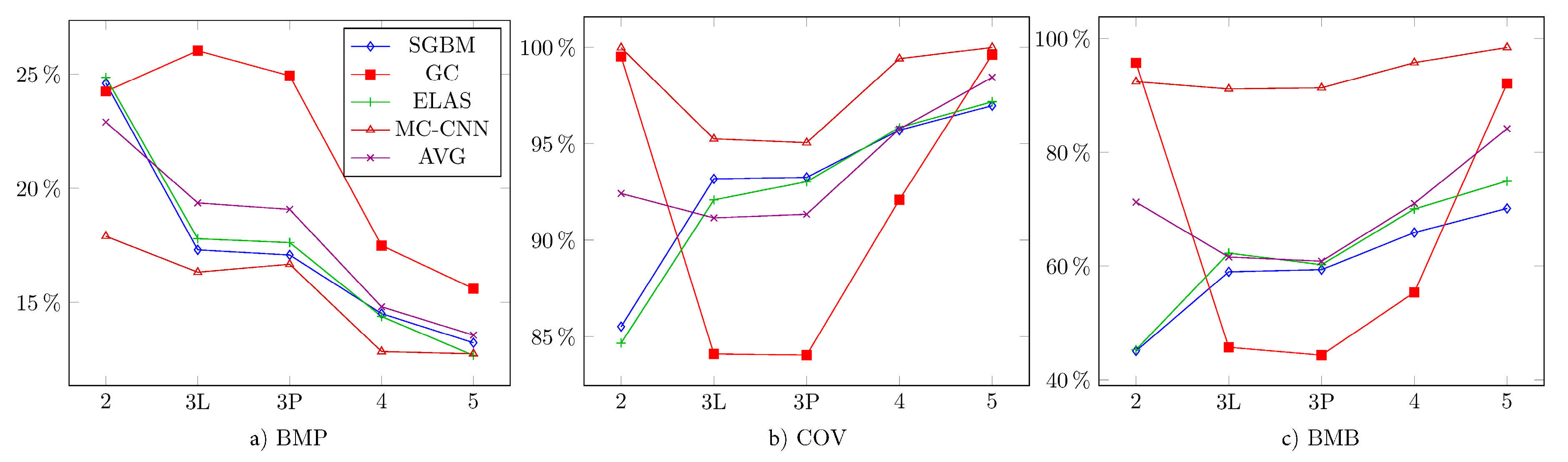
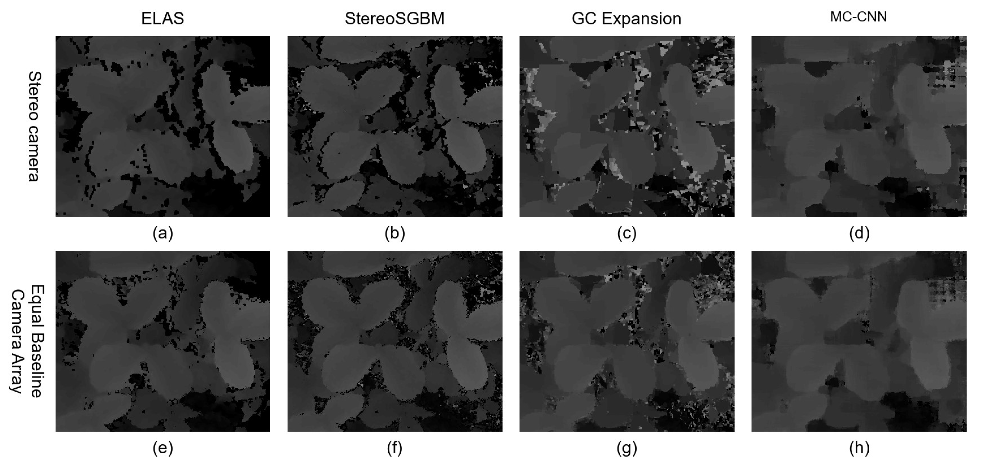
6.3. Different Number of Cameras

The EEMM method was originally designed for merging four disparity maps obtained with the use of four stereo cameras considered in EBCA. However, this paper describes the possibility of using the method with EBCA arrays in which the number of side cameras is lower than four. Merging less than four disparity maps can be perceived as merging four disparity maps such that there are blank maps in which all values of disparities are not determined.
The quality of results obtained by using Exception Excluding Merging Methods depends on the number of cameras included in EBCA as presented in Figure 12. Quality metrics considered in this section are the same as those considered in the previous section. The figure presents average results (AVG) and results for ELAS, GC Expansion, StereoSGBM and MC-CNN algorithms. Experiments were performed for the number of cameras ranging between two and five. Experimental sets differ in the number of side cameras. The same central camera was used in every configuration. Experimental data for tested arrays were acquired by removing images from a full set of images acquired from the array with all five cameras.
The usage of two cameras is equivalent to using a single stereo camera. There are four possibilities of obtaining such a configuration from the complete EBCA. In each case, a central camera and one of four side cameras is used. The results presented in Figure 12 were based on calculated the average mean of four different results obtained from four camera pairs possible to select from a set with five cameras. This kind of calculating the average mean of results obtained from all possible subsets was also applied in every other configuration.
Configuration 3P means that there are three cameras placed along a straight line. Such a configuration can be acquired from a complete EBCA set by selecting cameras located either along a horizontal line or along a vertical line. Configuration 3L also consists of three cameras however they are arranged in the L-configuration, i.e., cameras are in locations corresponding to vertices of a isosceles rectangular triangle. The purpose of distinguishing between configurations 3L and 3R is to verify whether differences in the arrangement of three-camera EBCA influence the quality of results. Configuration 4 is the one in which one camera was excluded from a full set of five cameras. Configuration 5 consists of all cameras used in the tested EBCA.
Figure 12 visualizes that the increase in the number of cameras reduces the value of the BMP metric, which means that the quality of results become higher. When two cameras are used, all tested stereo matching algorithms provided disparity maps with the value of BMP in the range between 17.9% and 24.85%. The greatest influence on the results caused by increasing the number of cameras occurred for the ELAS algorithm. The final result was equal to 12.68% with the use of five cameras. Thus, results improved 48.97% of its value obtained for a single pair of cameras. On average the improvement was equal to 40.79%. The MC-CNN algorithm produced results for which BMP was the lowest in the configuration with a single pair of cameras. These results were even further improved by increasing of the number of cameras included in the array. However, it was the ELAS algorithm which generated results with the lowest value of BMP when five cameras were used. Results for MC-CNN used with the same number of cameras were only slightly worse as the difference in values of BMP for these two algorithms was equal to 0.07%. These results show that applying a stereo matching algorithm to EBCA with five cameras can lead to satisfactory results even if results of this algorithm were poor when it was used with a stereo camera.
Moreover, there are not significant differences between configuration 3L and 3P. Therefore, it is insignificant on which side of a central camera a third camera is placed when a configuration with three cameras is used. Nevertheless, it is possible that in some circumstances one of these configurations is better depending on the shape or illumination of viewed objects.
The decrease in the value of BMP was associated with the increase in the value of the COV metric as shown in Figure 12b. This means that obtained disparity map contained overall less points for which disparities were not available. Charts obtained for GC and MC-CNN algorithms look peculiar because highest values were reported for two and five cameras. The reason is such that these algorithms provide data for almost all points of a disparity map when they are used with a stereo camera. Therefore, the COV metric for these algorithms drops when the EEMM is applied and the number of camera is increased to 3. Further increase in the number of cameras implies greater values of COV similarly as in case of SGBM and ELAS algorithms.
Figure 12c presents error rate for points located in the background. The BMB metric becomes greater in case of all algorithms when the number of cameras increases from three to four and from four to five. It corresponds to the increase in the values of the COV metric showing that disparity maps contain values of disparities in almost all points. In case of GC and MC-CNN algorithms, the error rate in background is nearly equal to 100% when two and five cameras are used because these algorithms provide values of disparities in areas of images which should be marked with values indicating that the disparity is unknown. For this reason, results of MC-CNN need to be considered worse than results of ELAS in the configuration with five cameras, although values of BMP indicate that the quality of these algorithm is similar. ELAS in much larger extent correctly identifies points for which disparities need to be marked as unknown. MC-CNN generates incorrect data for these areas.

7. EBCA Applications

The main application of Equal Baseline Camera Array is robotics. In particular, it can be applied to autonomous robots equipped with a robotic arm. Such robots can be used for manufacturing, quality assurance [13], agricultural applications or any operations requiring picking up objects in 3D space. EBCA can be even applied to robots designed for construction works such as paining walls in building [64].
Another major application of EBCA is providing 3D vision for autonomous cars [65]. Such vehicles operate in outdoor environment causing significant limitations in possibilities of using various kinds of 3D vision systems because intensive sunlight may interfere with measurements performed by these equipment.
EBCA can also be used for making 3D scans of objects covered with a semi-transparent material or made from this kind of substance [66]. Ihrke et al. presented a survey on this topic inducing making scans of smoke and objects made from glass [67]. The authors of this paper also performed experiments with 3D scanning of semi-transparent objects which were amber fossils with inclusions such as leaves [68].
A problem similar to 3D scanning of semi-transparent objects is enabling 3D vision for underwater operations [69]. Commonly used equipment for 3D scanning, such as structured light scanners, faces significant limitations when it is used for such a purpose. The array presented in this paper can be in particular applied to unmanned underwater vehicles and provide these devices with 3D vision. UUVs are remotely controlled and 3D vision of these devices supports their operators in performing expected tasks.
Drones are another kind of devices that can benefit from using EBCA [70]. Drones have a view over long distances in comparison to their size. Moreover, it is preferable to provide vision in high resolution. Obtaining high resolution for long distances cannot be achieved with LIDAR scanners or structured light scanners. However, cameras are suitable for such an application.
There is also an area of application of EBCA in a form of a 3D camera for general use. Users of such a camera can record videos similarly as they do using 2D cameras or their mobile phones. Nevertheless, popularizing such an application would have to be related with the growth of popularity and further development of 3D displays.

8. Conclusions

EBCA is a subject worth investigating due to its wide range of applications. The calibration technology presented in this paper makes it possible to assemble new EBCA which can be used by other researchers. Moreover, the testbed released as a part of presented research supports researchers in the development and testing of novel algorithms intended for obtaining disparity maps with the use of EBCA.
The most significant contribution presented in this paper is the calibration method which reduces the value of BMP metrics by over 34%. Another high value observation is the relation between number of cameras in EBCA and the quality of results when the EEMM merging method is used. Plans for future work include mounting EBCA on a robotic arm and performing hand–eye calibration.

Author Contributions

Conceptualization, A.L.K.; methodology, A.L.K.; software, A.L.K.; validation, A.L.K.; formal analysis, A.L.K. and B.B.; investigation, A.L.K.; resources, A.L.K. and B.B.; data curation, A.L.K.; writing—original draft preparation, A.L.K. and B.B.; writing—review and editing, A.L.K. and B.B.; visualization, A.L.K.; supervision, A.L.K.; project administration, A.L.K.; funding acquisition, A.L.K.; Overall A.L.K. 90%, B.B. 10%. All authors have read and agreed to the published version of the manuscript.

Funding

This work was supported in part under ministry subsidy for research for Gdansk University of Technology, Poland.

Institutional Review Board Statement

Not applicable.

Informed Consent Statement

Not applicable.

Data Availability Statement

The testbed and test data sets presented in this study are openly available at https://github.com/alkaczma/ebca (accessed on 9 August 2021).

Conflicts of Interest

The authors declare no conflict of interest.

Abbreviations

The following abbreviations are used in this manuscript:
EBCAEqual Baseline Camera Array
EEMMExceptions Excluding Merging Method
LIDARLight Detection and Ranging
TOFTime-of-flight camera
ELASEfficient Large-scale Stereo Matching
StereoSGBMStereo Semi-Global Block Matching
GC ExpansionGraph Cut with Expansion Moves
BMPpercentage of bad matching pixels
BMBpercentage of bad matching pixels in background
COVcoverage
SIFTscale-invariant feature transform
SURFspeeded up robust features
UUVunmanned underwater vehicle
CNNconvolutional neural network
MAmatching area
MRmargin area

References

  1. Park, J.I.; Inoue, S. Acquisition of sharp depth map from multiple cameras. Signal Process. Image Commun. 1998, 14, 7–19. [Google Scholar] [CrossRef]
  2. Kaczmarek, A.L. 3D Vision System for a Robotic Arm Based on Equal Baseline Camera Array. J. Intell. Robot. Syst. 2019, 99, 13–28. [Google Scholar] [CrossRef] [Green Version]
  3. Kaczmarek, A.L. Stereo vision with Equal Baseline Multiple Camera Set (EBMCS) for obtaining depth maps of plants. Comput. Electron. Agric. 2017, 135, 23–37. [Google Scholar] [CrossRef]
  4. Kaczmarek, A.L. Influence of Aggregating Window Size on Disparity Maps Obtained from Equal Baseline Multiple Camera Set (EBMCS). In Image Processing and Communications Challenges 8; Choraś, R.S., Ed.; Springer International Publishing: Cham, Switzerland, 2017; pp. 187–194. [Google Scholar]
  5. Kaczmarek, A.L. Stereo camera upgraded to equal baseline multiple camera set (EBMCS). In Proceedings of the 2017 3DTV Conference: The True Vision—Capture, Transmission and Display of 3D Video (3DTV-CON), Copenhagen, Denmark, 7–9 June 2017; pp. 1–4. [Google Scholar] [CrossRef]
  6. Ciurea, F.; Lelescu, D.; Chatterjee, P.; Venkataraman, K. Adaptive Geometric Calibration Correction for Camera Array. Electron. Imaging 2016, 2016, 1–6. [Google Scholar] [CrossRef]
  7. Furukawa, Y.; Ponce, J. Accurate camera calibration from multi-view stereo and bundle adjustment. Int. J. Comput. Vis. 2009, 84, 257–268. [Google Scholar] [CrossRef]
  8. Antensteiner, D.; Blaschitz, B. Multi-camera Array Calibration For Light Field Depth Estimation. In Proceedings of the Austrian Association for Pattern Recognition Workshop (OAGM), Hall in Tirol, Austria, 15–16 May 2018. [Google Scholar]
  9. Scharstein, D.; Szeliski, R.; Zabih, R. A taxonomy and evaluation of dense two-frame stereo correspondence algorithms. In Proceedings of the IEEE Workshop on Stereo and Multi-Baseline Vision (SMBV 2001), Kauai, HI, USA, 9–10 December 2001; pp. 131–140. [Google Scholar] [CrossRef]
  10. Scharstein, D.; Szeliski, R. A Taxonomy and Evaluation of Dense Two-Frame Stereo Correspondence Algorithms. Int. J. Comput. Vis. 2002, 47, 7–42. [Google Scholar] [CrossRef]
  11. Geiger, A.; Lenz, P.; Urtasun, R. Are we ready for autonomous driving? The KITTI vision benchmark suite. In Proceedings of the 2012 IEEE Conference on Computer Vision and Pattern Recognition, Providence, RI, USA, 16–21 June 2012; pp. 3354–3361. [Google Scholar] [CrossRef]
  12. Zbontar, J.; LeCun, Y. Stereo matching by training a convolutional neural network to compare image patches. J. Mach. Learn. Res. 2016, 17, 1–32. [Google Scholar]
  13. Traxler, L.; Ginner, L.; Breuss, S.; Blaschitz, B. Experimental Comparison of Optical Inline 3D Measurement and Inspection Systems. IEEE Access 2021, 9, 53952–53963. [Google Scholar] [CrossRef]
  14. Jang, W.; Je, C.; Seo, Y.; Lee, S.W. Structured-light stereo: Comparative analysis and integration of structured-light and active stereo for measuring dynamic shape. Opt. Lasers Eng. 2013, 51, 1255–1264. [Google Scholar] [CrossRef]
  15. Rasul, A.; Seo, J.; Khajepour, A. Development of Sensing Algorithms for Object Tracking and Predictive Safety Evaluation of Autonomous Excavators. Appl. Sci. 2021, 11, 6366. [Google Scholar] [CrossRef]
  16. Yim, J.H.; Kim, S.Y.; Kim, Y.; Cho, S.; Kim, J.; Ahn, Y.H. Rapid 3D-Imaging of Semiconductor Chips Using THz Time-of-Flight Technique. Appl. Sci. 2021, 11, 4770. [Google Scholar] [CrossRef]
  17. Seitz, S.M.; Curless, B.; Diebel, J.; Scharstein, D.; Szeliski, R. A Comparison and Evaluation of Multi-View Stereo Reconstruction Algorithms. In Proceedings of the 2006 IEEE Computer Society Conference on Computer Vision and Pattern Recognition (CVPR’06), New York, NY, USA, 17–22 June 2006; Volume 1, pp. 519–528. [Google Scholar] [CrossRef]
  18. Antensteiner, D.; Štolc, S.; Valentín, K.; Blaschitz, B.; Huber-Mörk, R.; Pock, T. High-precision 3d sensing with hybrid light field & photometric stereo approach in multi-line scan framework. Electron. Imaging 2017, 2017, 52–60. [Google Scholar]
  19. Okutomi, M.; Kanade, T. A multiple-baseline stereo. Pattern Anal. Mach. Intell. IEEE Trans. 1993, 15, 353–363. [Google Scholar] [CrossRef]
  20. Wilburn, B.; Joshi, N.; Vaish, V.; Talvala, E.V.; Antunez, E.; Barth, A.; Adams, A.; Horowitz, M.; Levoy, M. High Performance Imaging Using Large Camera Arrays; ACM SIGGRAPH 2005 Papers; ACM: New York, NY, USA, 2005; pp. 765–776. [Google Scholar] [CrossRef]
  21. Wang, D.; Pan, Q.; Zhao, C.; Hu, J.; Xu, Z.; Yang, F.; Zhou, Y. A Study on Camera Array and Its Applications. IFAC-PapersOnLine 2017, 50, 10323–10328. [Google Scholar] [CrossRef]
  22. Manta, A. Multiview Imaging and 3D TV. A Survey; Delft University of Technology, Information and Communication Theory Group: Delft, The Netherlands, 2008. [Google Scholar]
  23. Nalpantidis, L.; Gasteratos, A. Stereo Vision Depth Estimation Methods for Robotic Applications. In Depth Map and 3D Imaging Applications: Algorithms and Technologies; IGI Global: Hershey, PA, USA, 2011; Volume 3, pp. 397–417. [Google Scholar] [CrossRef]
  24. Ackermann, M.; Cox, D.; McGraw, J.; Zimmer, P. Lens and Camera Arrays for Sky Surveys and Space Surveillance. In Proceedings of the Advanced Maui Optical and Space Surveillance Technologies Conference, Wailea, HI, USA, 20–23 September 2016. [Google Scholar]
  25. Venkataraman, K.; Lelescu, D.; Duparré, J.; McMahon, A.; Molina, G.; Chatterjee, P.; Mullis, R.; Nayar, S. PiCam: An Ultra-thin High Performance Monolithic Camera Array. ACM Trans. Graph. 2013, 32, 166:1–166:13. [Google Scholar] [CrossRef] [Green Version]
  26. Ge, K.; Hu, H.; Feng, J.; Zhou, J. Depth Estimation Using a Sliding Camera. IEEE Trans. Image Process. 2016, 25, 726–739. [Google Scholar] [CrossRef] [PubMed]
  27. Xiao, X.; Daneshpanah, M.; Javidi, B. Occlusion Removal Using Depth Mapping in Three-Dimensional Integral Imaging. J. Disp. Technol. 2012, 8, 483–490. [Google Scholar] [CrossRef]
  28. Hensler, J.; Denker, K.; Franz, M.; Umlauf, G. Hybrid Face Recognition Based on Real-Time Multi-camera Stereo-Matching. In Lecture Notes in Computer Science, Proceedings of the Advances in Visual Computing, Las Vegas, NV, USA, 26–28 September 2011; Springer: Berlin/Heidelberg, Germany, 2011; Volume 6939, pp. 158–167. [Google Scholar] [CrossRef] [Green Version]
  29. Ayache, N.; Lustman, F. Trinocular stereo vision for robotics. IEEE Trans. Pattern Anal. Mach. Intell. 1991, 13, 73–85. [Google Scholar] [CrossRef]
  30. Mulligan, J.; Kaniilidis, K. Trinocular stereo for non-parallel configurations. In Proceedings of the 15th International Conference on Pattern Recognition, ICPR-2000, Barcelona, Spain, 3–7 September 2000; Volume 1, pp. 567–570. [Google Scholar] [CrossRef] [Green Version]
  31. Mulligan, J.; Isler, V.; Daniilidis, K. Trinocular Stereo: A Real-Time Algorithm and its Evaluation. Int. J. Comput. Vis. 2002, 47, 51–61. [Google Scholar] [CrossRef]
  32. Andersen, J.C.; Andersen, N.A.; Ravn, O. Trinocular stereo vision for intelligent robot navigation. In Proceedings of the IFAC/EURON Symposium on Intelligent Autonomous Vehicles, Lisbon, Portugal, 5–7 July 2004. [Google Scholar] [CrossRef] [Green Version]
  33. Williamson, T.; Thorpe, C. A trinocular stereo system for highway obstacle detection. In Proceedings of the 1999 IEEE International Conference on Robotics and Automation (Cat. No.99CH36288C), Detroit, MI, USA, 10–15 May 1999; Volume 3, pp. 2267–2273. [Google Scholar] [CrossRef]
  34. Wang, J.; Xiao, X.; Javidi, B. Three-dimensional integral imaging with flexible sensing. Opt. Lett. 2014, 39, 6855–6858. [Google Scholar] [CrossRef]
  35. Scharstein, D.; Hirschmüller, H.; Kitajima, Y.; Krathwohl, G.; Nešić, N.; Wang, X.; Westling, P. High-Resolution Stereo Datasets with Subpixel-Accurate Ground Truth. In Proceedings of the Pattern Recognition: 36th German Conference, GCPR 2014, Münster, Germany, 2–5 September 2014; Springer International Publishing: Cham, Switzerland, 2014; pp. 31–42. [Google Scholar] [CrossRef] [Green Version]
  36. Menze, M.; Heipke, C.; Geiger, A. Joint 3D Estimation of Vehicles and Scene Flow. In Proceedings of the ISPRS Annals of the Photogrammetry, Remote Sensing and Spatial Information Sciences, Volume II-3W5, La Grande Motte, France, 28 September–3 October 2015. ISPRS: Hannover, Germany, 2015; pp. 427–434. [Google Scholar]
  37. Silberman, N.; Hoiem, D.; Kohli, P.; Fergus, R. Indoor Segmentation and Support Inference from RGBD Images. In Lecture Notes in Computer Science, Proceedings of the ECCV 2012, Florence, Italy, 7–13 October 2012; Springer: Berlin/Heidelberg, Germany, 2012; Volume 7576. [Google Scholar] [CrossRef]
  38. Schöps, T.; Schönberger, J.L.; Galliani, S.; Sattler, T.; Schindler, K.; Pollefeys, M.; Geiger, A. A Multi-View Stereo Benchmark with High-Resolution Images and Multi-Camera Videos. In Proceedings of the IEEE Proceedings of the Conference on Computer Vision and Pattern Recognition (CVPR), Honolulu, HI, USA, 21–26 July 2017; pp. 2538–2547. [Google Scholar] [CrossRef]
  39. Geiger, A.; Roser, M.; Urtasun, R. Efficient Large-Scale Stereo Matching. In Lecture Notes in Computer Science, Proceedings of the Computer Vision—ACCV 2010 10th Asian Conference on Computer Vision, Queenstown, New Zealand, 8–12 November 2010; Kimmel, R., Klette, R., Sugimoto, A., Eds.; Springer: Berlin/Heidelberg, Germany, 2011; Volume 6492, pp. 25–38. [Google Scholar] [CrossRef]
  40. Hirschmuller, H. Stereo Processing by Semiglobal Matching and Mutual Information. Pattern Anal. Mach. Intell. IEEE Trans. 2008, 30, 328–341. [Google Scholar] [CrossRef]
  41. Bradski, D.G.R.; Kaehler, A. Learning Opencv, 1st ed.; O’Reilly Media, Inc.: Sebastopol, CA, USA, 2008. [Google Scholar]
  42. Boykov, Y.; Veksler, O.; Zabih, R. Fast approximate energy minimization via graph cuts. Pattern Anal. Mach. Intell. IEEE Trans. 2001, 23, 1222–1239. [Google Scholar] [CrossRef] [Green Version]
  43. Besag, J. On the Statistical Analysis of Dirty Pictures. J. R. Stat. Soc. Ser. B (Methodol.) 1986, 48, 259–302. [Google Scholar] [CrossRef] [Green Version]
  44. Goodfellow, I.; Bengio, Y.; Courville, A. Deep Learning; MIT Press: Cambridge, MA, USA, 2016; Available online: http://www.deeplearningbook.org (accessed on 9 August 2021).
  45. Hartley, R.; Zisserman, A. Multiple View Geometry in Computer Vision, 2nd ed.; Cambridge University Press: Cambridge, UK, 2004. [Google Scholar] [CrossRef] [Green Version]
  46. Blaschitz, B.; Štolc, S.; Antensteiner, D. Geometric calibration and image rectification of a multi-line scan camera for accurate 3d reconstruction. In Proceedings of the IS&T International Symposium on Electronic Imaging, Burlingame, CA, USA, 28 January–1 February 2018. IS&T: Springfield, VA, USA, 2018; pp. 240-1–240-6. [Google Scholar] [CrossRef]
  47. Tao, J.; Wang, Y.; Cai, B.; Wang, K. Camera Calibration with Phase-Shifting Wedge Grating Array. Appl. Sci. 2018, 8, 644. [Google Scholar] [CrossRef] [Green Version]
  48. Kang, Y.S.; Ho, Y.S. An efficient image rectification method for parallel multi-camera arrangement. Consum. Electron. IEEE Trans. 2011, 57, 1041–1048. [Google Scholar] [CrossRef]
  49. Yang, J.; Guo, F.; Wang, H.; Ding, Z. A multi-view image rectification algorithm for matrix camera arrangement. In Artificial Intelligence Research; Sciedu Press: Richmond Hill, ON, Canada, 2014; Volume 3, pp. 18–29. [Google Scholar] [CrossRef]
  50. Sun, C. Uncalibrated three-view image rectification. Image Vis. Comput. 2003, 21, 259–269. [Google Scholar] [CrossRef]
  51. Hartley, R.I. Theory and Practice of Projective Rectification. Int. J. Comput. Vis. 1999, 35, 115–127. [Google Scholar] [CrossRef]
  52. Hosseininaveh, A.; Serpico, M.; Robson, S.; Hess, M.; Boehm, J.; Pridden, I.; Amati, G. Automatic Image Selection in Photogrammetric Multi-view Stereo Methods. In Proceedings of the 13th International Symposium on Virtual Reality, Archaeology and Cultural Heritage VAST, Brighton, UK, 19–21 November 2012; Eurographics Association: Geneve, Switzerland, 2012; pp. 9–16. [Google Scholar]
  53. Lowe, D. Object recognition from local scale-invariant features. In Proceedings of the Seventh IEEE International Conference on Computer Vision, Kerkyra, Greece, 20–27 September 1999; Volume 2, pp. 1150–1157. [Google Scholar] [CrossRef]
  54. Liu, R.; Zhang, H.; Liu, M.; Xia, X.; Hu, T. Stereo Cameras Self-Calibration Based on SIFT. In Proceedings of the 2009 International Conference on Measuring Technology and Mechatronics Automation, Zhangjiajie, China, 11–12 April 2009; Volume 1, pp. 352–355. [Google Scholar] [CrossRef]
  55. Bay, H.; Ess, A.; Tuytelaars, T.; Gool, L.V. Speeded-Up Robust Features (SURF). Comput. Vis. Image Underst. 2008, 110, 346–359. [Google Scholar] [CrossRef]
  56. Boukamcha, H.; Atri, M.; Smach, F. Robust auto calibration technique for stereo camera. In Proceedings of the 2017 International Conference on Engineering MIS (ICEMIS), Monastir, Tunisia, 8–10 May 2017; pp. 1–6. [Google Scholar] [CrossRef]
  57. Mentzer, N.; Mahr, J.; Payá-Vayá, G.; Blume, H. Online stereo camera calibration for automotive vision based on HW-accelerated A-KAZE-feature extraction. J. Syst. Archit. 2019, 97, 335–348. [Google Scholar] [CrossRef]
  58. Carrera, G.; Angeli, A.; Davison, A.J. SLAM-based automatic extrinsic calibration of a multi-camera rig. In Proceedings of the 2011 IEEE International Conference on Robotics and Automation, Shanghai, China, 9–13 May 2011; pp. 2652–2659. [Google Scholar] [CrossRef] [Green Version]
  59. Heng, L.; Bürki, M.; Lee, G.H.; Furgale, P.; Siegwart, R.; Pollefeys, M. Infrastructure-based calibration of a multi-camera rig. In Proceedings of the 2014 IEEE International Conference on Robotics and Automation (ICRA), Hong Kong, China, 31 May–5 June 2014; pp. 4912–4919. [Google Scholar] [CrossRef]
  60. Fehrman, B.; McGough, J. Depth mapping using a low-cost camera array. In Proceedings of the 2014 Southwest Symposium on Image Analysis and Interpretation, San Diego, CA, USA, 6–8 April 2014; pp. 101–104. [Google Scholar] [CrossRef]
  61. Fehrman, B.; McGough, J. Handling occlusion with an inexpensive array of cameras. In Proceedings of the 2014 Southwest Symposium on Image Analysis and Interpretation, San Diego, CA, USA, 6–8 April 2014; pp. 105–108. [Google Scholar] [CrossRef]
  62. Kaczmarek, A.L. Improving depth maps of plants by using a set of five cameras. J. Electron. Imaging 2015, 24, 023018. [Google Scholar] [CrossRef] [Green Version]
  63. Zhang, Z. A flexible new technique for camera calibration. IEEE Trans. Pattern Anal. Mach. Intell. 2000, 22, 1330–1334. [Google Scholar] [CrossRef] [Green Version]
  64. Tadic, V.; Odry, A.; Burkus, E.; Kecskes, I.; Kiraly, Z.; Klincsik, M.; Sari, Z.; Vizvari, Z.; Toth, A.; Odry, P. Painting Path Planning for a Painting Robot with a RealSense Depth Sensor. Appl. Sci. 2021, 11, 1467. [Google Scholar] [CrossRef]
  65. Zaarane, A.; Slimani, I.; Al Okaishi, W.; Atouf, I.; Hamdoun, A. Distance measurement system for autonomous vehicles using stereo camera. Array 2020, 5, 100016. [Google Scholar] [CrossRef]
  66. Kopf, C.; Pock, T.; Blaschitz, B.; Štolc, S. Inline Double Layer Depth Estimation with Transparent Materials. In Lecture Notes in Computer Science, Proceedings of the Pattern Recognition: 42nd DAGM German Conference, DAGM GCPR 2020, Tübingen, Germany, 28 September–1 October 2020; Springer International Publishing: Cham, Switzerland, 2021; pp. 418–431. [Google Scholar]
  67. Ihrke, I.; Kutulakos, K.N.; Lensch, H.P.A.; Magnor, M.; Heidrich, W. Transparent and Specular Object Reconstruction. Comput. Graph. Forum 2010, 29, 2400–2426. [Google Scholar] [CrossRef]
  68. Kaczmarek, A.L.; Lebiedź, J.; Jaroszewicz, J.; Świȩszkowski, W. 3D Scanning of Semitransparent Amber with and without Inclusions. In Proceedings of the International Conference in Central Europe on Computer Graphics, Visualization and Computer Vision WSCG 2021, Pilsen, Czech Republic, 17–20 May 2021; pp. 145–154. [Google Scholar] [CrossRef]
  69. Watson, S.; Duecker, D.A.; Groves, K. Localisation of Unmanned Underwater Vehicles (UUVs) in Complex and Confined Environments: A Review. Sensors 2020, 20, 6203. [Google Scholar] [CrossRef] [PubMed]
  70. Fanta-Jende, P.; Steininger, D.; Bruckmüller, F.; Sulzbachner, C. A Versatile Uav near real-time mapping solution for disaster response—Concept, ideas and implementation. Int. Arch. Photogramm. Remote Sens. Spat. Inf. Sci. 2020, 43, 429–435. [Google Scholar] [CrossRef]
Figure 1. A sample set of images taken by a four camera rig (two stereo cameras placed side by side) used in ETH3D Benchmark, (a) the left image from the left stereo camera, (b) the right image from the left stereo camera, (c) the left image from the right stereo camera, (d) the right image from the right stereo camera.
Applsci 11 08464 g001
Figure 2. AIT’s dot pattern calibration target with 3-dot central element (left: abstract representation, right: actual acquisition with one of EBCA’s caneras). Note that this pattern is the smallest possible asymmetric configuration on a regular grid and three distinct marks (the different color is for illustration only) suffice to estimate an affine transformation, which approximates the more general perspective transformation needed to unwarp the image, c.f. [46] for details.
Applsci 11 08464 g002
Figure 3. The camera set consisting of MS LifeCam Studio mounted in the form of Equal Baseline Camera Array.
Applsci 11 08464 g003
Figure 4. The process of stereo matching using pairwise calibration.
Applsci 11 08464 g004
Figure 5. Images taken by EBCA used for creating data set of strawberry images: (a) central image, (b) right image, (c) up image, (d) left image and (e) bottom image.
Applsci 11 08464 g005
Figure 6. Pairs of images in strawberry data set S T 1 after performing the calibration process. (a,b) The left pair, (c,d) The up pair. (e,f) The right pair. (g,h) The bottom pair.
Applsci 11 08464 g006
Figure 7. The comparison between results based on images without self-calibration and results based on images with self-calibration.
Applsci 11 08464 g007
Figure 8. Values of the BMP metric when EEMM was used with algorithms: (a) ELAS, (b) StereoSGBM, (c) GC Expansion and (d) MC-CNN.
Applsci 11 08464 g008
Figure 9. Values of the BMB metric when EEMM was used with algorithms: (a) ELAS, (b) StereoSGBM, (c) GC Expansion and (d) MC-CNN.
Applsci 11 08464 g009
Figure 10. Values of the COV metric when EEMM was used with algorithms: (a) ELAS, (b) StereoSGBM, (c) GC Expansion and (d) MC-CNN.
Applsci 11 08464 g010
Figure 11. Disparity maps obtained using a pair of cameras (ad) and EBCA (eh) for the following stereo matching algorithms: ELAS (a,e), StereoSGBM (b,f), GC Expansion (c,g) and MC-CNN (d,h).
Applsci 11 08464 g011
Figure 12. Results obtained for EEMM used with different number of cameras. The figure presents values of the following quality metrics: (a) BMP, (b) COV and (c) BMB.
Applsci 11 08464 g012
Table 1. Sizes of test data sets and the range of disparities.
Set IDMatching SizeDisparity Range
S T 1 440 × 3801–28
S T 2 340 × 32519–45
R C 1 420 × 37031–79
R C 2 320 × 29511–35
C H 1 470 × 38040–69
C H 2 330 × 31027–58
Publisher’s Note: MDPI stays neutral with regard to jurisdictional claims in published maps and institutional affiliations.

