A Coupled Multiscale Approach to Modeling Aortic Valve Mechanics in Health and Disease

Abstract

Mechano-biological processes in the aortic valve span multiple length scales ranging from the molecular and cell to tissue and organ levels. The valvular interstitial cells residing within the valve cusps sense and actively respond to leaflet tissue deformations caused by the valve opening and closing during the cardiac cycle. Abnormalities in these biomechanical processes are believed to impact the matrix-maintenance function of the valvular interstitial cells, thereby initiating valvular disease processes such as calcific aortic stenosis. Understanding the mechanical behavior of valvular interstitial cells in maintaining tissue homeostasis in response to leaflet tissue deformation is therefore key to understanding the function of the aortic valve in health and disease. In this study, we applied a multiscale computational homogenization technique (also known as “FE${}^2$”) to aortic valve leaflet tissue to study the three-dimensional mechanical behavior of the valvular interstitial cells in response to organ-scale mechanical loading. We further considered calcific aortic stenosis with the aim of understanding the likely relationship between the valvular interstitial cell deformations and calcification. We find that the presence of calcified nodules leads to an increased strain profile that drives further growth of calcification.

1. Introduction and Objective

Mechanotransduction is the process by which living cells and tissues respond to mechanical stimuli and activate biochemical pathways that influence a variety of intracellular and extracellular biological functions. These processes span a wide spectrum of length scales ranging from the molecular and sub-cellular to the tissue and organ levels. Due to the importance of microscale behavior in biological systems, traditional biomechanical modeling is limited in its capabilities. Multiscale modeling techniques, such as computational homogenization (also known as “FE${}^2$”), however, can be used to investigate the micromechanical behavior of cells in biological systems, and hence mechanotransduction. Such an approach is important for developing heart valve biomechanical models that capture the essential roles of valvular interstitial cells in maintaining tissue homoestasis and regulating pathology.

The aortic valve (AV) is the gateway for the delivery of pressurized, oxygenated blood from the left ventricle to the aorta and thereby the rest of the body [1]. The function of the AV in health and disease directly involves processes occurring at the cellular scale. Biochemical pathways are activated from mechanical feedback loops between the valvular interstitial cells (VICs) and the AV leaflet tissue [2,3]. Shape changes in valvular interstitial cells (VICs), particularly the aspect ratios, have been proposed as a measure of cellular mechanotransduction activity. Experiments have been performed by several laboratories that investigated this metric in response to the physiological loading of aortic valve leaflet tissue. In an effort to better understand the nature of AV disease, researchers have been exploring the central role of VICs by modeling the inherently multiscale behavior of AV tissue [4,5,6,7]. Numerical simulations that mimic these experiments were carried out but were limited to 2D and uncoupled 3D models (i.e., no interaction between the macroscale and microscale).

Weinberg et al. [6,8,9] developed the first 3D, multiscale, transient model of the aortic valve in health and disease, where they coupled the organ-level (whole valve) mechanical strains to tissue and cell-level events, and found agreeable results to the ex vivo experiments that related whole valve deformations to VIC deformations. Missing from the literature, however, are fully coupled multiscale models, i.e., models that allow for two-way interaction between the disparate length scales. Naturally, a meaningful model of the full resolution of the AV, incorporating the cells that make up its microstructure, is a computationally intractable problem. An alternative is computational homogenization, sometimes known as FE${}^2$, where a statistical representation of the microstructure (the “representative volume element” or RVE) is embedded into a macroscale model.

Computational homogenization is a viable way of coupling multiscale behavior [10]. We use this approach to study the valvular interstitial cell’s aspect ratio (VICAR) as a representation of cellular deformations. VICAR is defined as the ratio of the valvular interstitial cell’s longest length dimension to its shortest, and it is often used as a suitable metric for cellular shape changes, i.e., the stimuli for mechanotransduction, as proposed by Huang [4]. We are able identify that the perceived aspect ratio from experiments may not be consistent with the actual 3D VIC deformations. With this methodology, we introduce a framework for more complex multiscale and multiphysics AV models.

The objective of this study was to apply FE${}^2$ to aortic valve leaflet tissue in 3D to study the mechanical behavior of the VIC in response to organ-scale mechanical loading. The modeling scheme importantly utilizes self-consistent material models based on layer-wise experimental data from aortic valve tissue. Our simulations demonstrate a viable method for the fully multiscale modeling of aortic valve tissue. We find that the “apparent” VIC aspect ratio observed in experiments may not necessarily be consistent with the actual 3D deformations of the cells. We further consider calcific aortic stenosis, the most prevalent aortic valve disease featuring the calcification of the valve leaflet tissues [11]. The aim here was to understand the relationship between the VIC aspect ratios and calcification. We find behavior that is consistent with previous single-scale studies in the literature, namely that the presence of calcified nodules leads to an increased strain profile that drives the further growth of calcification.

Aortic valve function: details regarding AV physiology may be found, e.g., in [12]. We briefly revisit them here. The AV complex consists of the aortic root, the sinus, the leaflets, and the ascending aorta, as depicted in Figure 1. Our main focus here are the leaflets (or cusps), shown in color in Figure 1.

Healthy AVs have three leaflets that open and close to allow blood flow from the ventricle into the ascending aorta and prevent retrograde flow. During the cardiac cycle (illustrated in Figure 2), blood flows in from the left atrium into the left ventricle during diastole, and the AV leaflets open (close) at the beginning (end) of systole.

Huang carried out a series of in vitro experiments to measure the VICAR in response to AV tissue loading during the cardiac cycle. AV leaflet samples were fixed in a tank and a pressure head was applied at five different levels, as shown in

Table 1. Pressure loading protocol in mmHg.

Load Step	1	2	3	4	5
Pressure	1	2	4	60	90

. Note that, in [4], the maximum pressure used was 90 mmHg; thus, for comparison purposes, all of our computations were also carried out to this pressure, as opposed to the conventional normal systolic pressure of 120 mmHg. The average VICAR was then measured at each pressure by image processing procedures of sections through the tissue thickness. Huang notes that the VICAR reported was the observed value, i.e., the apparent 2D elliptical aspect ratio that, in general, is not concentric with the presumed ellipsoidal shape. Further details regarding the experimental procedure can be found in [4]. Note that the net pressure load is on the aortic side of the leaflet. Physiologically, this corresponds to the period between the systole and diastole (Figure 2), right after the valve closes and the transvalvular pressure is the greatest.

Aortic valve tissue calcification: calcified aortic stenosis (CAS) is the most prevalent aortic valve (AV) disease, affecting approximately 25% of adults over 65 years of age [14]. It is characterized by a failure of the valve leaflets to fully open due to the formation of calcified lesions similar to bone tissue [15].

The calcification process is hypothesized to begin with the differentiation of the valvular interstitial cell (VIC) phenotype into osteoblast-like cells that alter the structure of the extracellular matrix (ECM) [16]. The calcified lesions begin as nodules that grow into non-random patterns [9]. A few common patterns have been identified, with the two most common being the “arc” and “partial arc” patterns (Figure 3) [17,18]. Halevi et al. [18] used reverse computed tomography (CT) to classify these patterns and how they progressed temporally and spatially. The calcification occurs more frequently on the aortic side of the valve (fibrosa) and the stiffening results in altered valve function [19,20,21,22].

The underlying cause of calcification is still under investigation, however, tissue strain and hemodynamic shear stresses have been identified as important biomechanical factors driving their growth [23,24,25,26,27]. These factors result in a biochemical signaling processes between the endothelial cells and the VICs, promoting VIC differentiation into a calcific phenotype [28].

Multiscale modeling: in an effort to capture the multiscale feedback inherent to the behavior of AV tissue in health and disease, we will introduce a full 3D coupled multiscale model via FE${}^2$. We first detail the theory and implementation of the model. Then, we calibrate the tissue model to the experimental data. We use the calibrated data to study VIC behavior in response to macroscale pressure loading in two states: healthy and calcified. We further investigate different stages of diseased valves, as mentioned above, to study the evolution of calcification in the tissue. The calcified states are considered by introducing regions of the tissue along the aortic face of the valve leaflet with material properties representing calcification in patterns similar to those observed in the diseased valves. We are able to identify a clear change in the VIC behavior in the non-calcified regions of the tissue which form a basis for the further progression and saturation of the calcified tissue.

2. Materials and Methods

In this section, we present our multiscale modeling approach (cf. Figure 4). We begin by introducing a continuum mechanics framework and then develop a finite element discretization to solve the governing equations. Finally, we contextualize the approach to the AV tissue model.

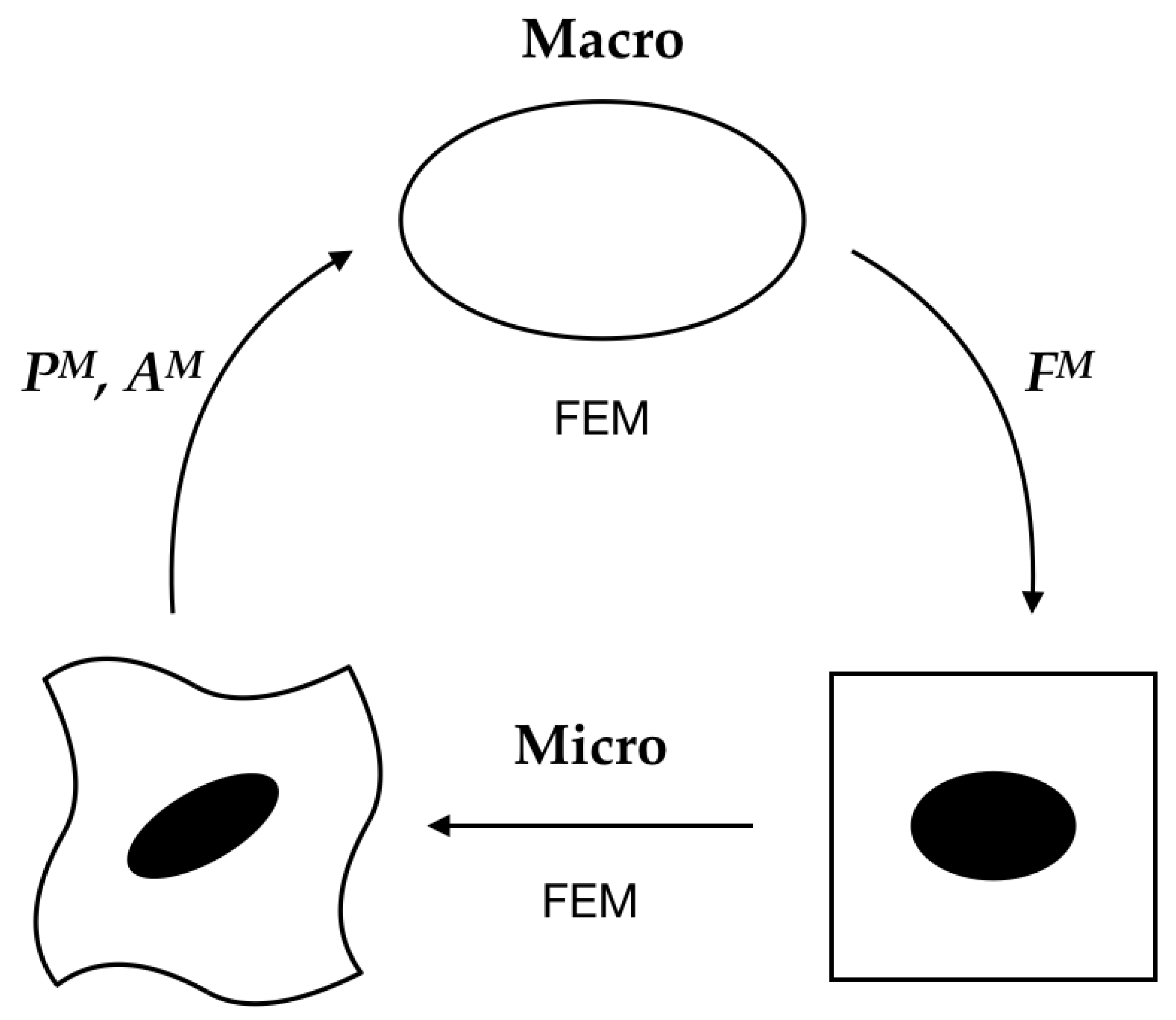
2.1. Multiscale Modeling Framework

We modeled the AV tissue within a classical continuum mechanics framework (see e.g., [29] or [30]), wherein we seek to solve the governing equations of motion for a body, i.e., the manifold with boundaries, subject to boundary conditions, specifying tractions and displacements. We define a one-parameter (time t) family of finite deformation maps ${\mathit{\phi }}_t:{\mathbb{R}}^3\mapsto {\mathbb{R}}^3$ of a hyperelastic body from a reference configuration (${\mathcal{B}}_0$) to a current (deformed) configuration (${\mathcal{B}}_t$) (see Fung [31] or Holzapfel [29]); viz., ${\mathcal{B}}_t={\mathit{\phi }}_t\left({\mathcal{B}}_0\right)$.

We define the deformation gradient $\mathit{F}=\nabla \mathit{\phi }$. Note that $\mathit{F}$ is a 2-point tensor mapping vectors from the reference manifold to the deformed manifold. We define the left and right Cauchy–Green deformation tensors by $\mathit{C}={\mathit{F}}^T\mathit{F}$ and $\mathit{b}=\mathit{F}{\mathit{F}}^T$, respectively. We further define the associated strain tensors: the Green–Lagrange strain tensor $\mathit{E}=\frac{1}{2}(\mathit{C}-\mathit{I})$ for the reference configuration and the Almansi strain tensor $\mathit{e}=\frac{1}{2}(\mathit{I}-{\mathit{b}}^{-1})$ for the current configuration. $\mathit{I}$ is the identity tensor for vectors in ${\mathbb{R}}^3$.

The equilibrium deformation map at time t is the one that minimizes the potential energy ($\mathsf{\Pi }$) of the elastic system subject to conservative traction loading ${\overline{\mathit{t}}}_t$:

$${\mathit{\phi }}_t^{eq}=arg\underset{{\mathit{\phi }}_t}{inf}\mathsf{\Pi }({\mathit{\phi }}_t;{\overline{\mathit{t}}}_t).$$

(1)

Under the assumption of hyperelasticity, the 1st Piola–Kirchhoff stress of the system, $\mathit{P}$, is obtained from the Helmholtz free energy, $\widehat{\psi }$, of the material:

$$\mathit{P}={\displaystyle \frac{\partial \widehat{\psi }}{\partial \mathit{F}}}.$$

(2)

Although the solution to (1) is in general not unique, the polyconvexity (in the sense of Ball [32] along with suitable growth conditions) of the energy function guarantees the existence of a solution. We solve the problem with a standard finite element (FE) numerical procedure (Section 2.1). Our challenge is to specify $\widehat{\psi }$ such that the FE model is consistent with the observed experimental response.

We can further define two additional stress tensors: the 2nd Piola–Kirchhoff stress tensor $\mathit{S}$ and the Cauchy stress tensor $\mathit{T}$. The relationship between the stress tensors is:

$$\mathit{T}=J^{-1}\mathit{F}\mathit{P}=J^{-1}\mathit{F}\mathit{S}{\mathit{F}}^T,$$

(3)

where $J=det\left(\mathit{F}\right)$ is the Jacobian (of the deformation gradient).

To use an FE approach to solve (1), let $\partial {\mathcal{B}}_u$ and $\partial {\mathcal{B}}_t$ denote the partitions of the boundary ($\partial {\mathcal{B}}_0$) of the body, ${\mathcal{B}}_0$, where deformation and tractions are imposed, respectively, with $\partial {\mathcal{B}}_u\cap \partial {\mathcal{B}}_t=\varnothing$, $\overline{\partial {\mathcal{B}}_u\cup \partial {\mathcal{B}}_t}=\partial {\mathcal{B}}_0$. Equation (1) is solved by satisfying the weak form statement:

Find:

$$\mathit{\phi }\in \mathcal{S}:=\left\{\mathit{\phi }\right|\mathit{\phi }=\overline{\mathit{\phi }}\mathrm{on}\partial {\mathcal{B}}_u\},$$

such that:

$${\int }_{{\mathcal{B}}_0}\mathit{P}·\nabla \left(\delta \mathit{\phi }\right)dV=\cancel{{\int }_{{\mathcal{B}}_0}\mathit{B}·\delta \mathit{\phi }dV}+{\int }_{\partial {\mathcal{B}}_t}\overline{\mathit{t}}·\delta \mathit{\phi }dA,$$

(4)

$$\forall \delta \mathit{\phi }\in \mathcal{V}:=\left\{\delta \mathit{\phi }\right|\delta \mathit{\phi }=\mathbf{0}\mathrm{on}{\mathcal{B}}_u\},$$

where we assume there is no body force $\mathit{B}$. The FE solution begins with a tessellation of the domain (cf. Figure 5) into a finite set of discrete nodes and elements. Letting the superscript g denote discretized parameters, and $N^A\left(\mathit{x}\right)$ denote interpolating shape functions at each node, we construct a Galerkin discretization as

$${\mathcal{B}}_0^h=\underset{e=1}{\overset{n_{el}}{\mathbf{A}}}{\mathcal{B}}_0^e,{\mathit{u}}^g=\sum _{A=1}^{n_n}{N}^A{\mathit{u}}_A,\delta {\mathit{u}}^g=\sum _{A=1}^{n_n}{N}^A\delta {\mathit{u}}_A,$$

(5)

where e indexes the $n_{el}$ elements in the domain, $\mathit{u}$ denotes displacements, $\delta \mathit{u}$ denotes variational displacements, ${\mathit{u}}_A$ denotes nodal displacements indexed by A over $n_n$ nodes in the tessellation, and $\underset{e=1}{\overset{n_{el}}{\mathbf{A}}}$ is the assembly operator [33]. Substituting (5) into (4) leads to the nonlinear (static) equilibrium equations:

$$\mathit{R}\left({\mathit{u}}_t\right)={\mathit{f}}_t-\underset{e=1}{\overset{n_{el}}{\mathbf{A}}}{\int }_{{\mathcal{B}}_0^e}\nabla {\mathit{N}}_e^T{\mathit{P}}_{e}d{V}_e=0,$$

(6)

where $\mathit{R}$ is the residual for a state of displacements ${\mathit{u}}_t$ at time t, which must be in equilibrium with the applied nodal forces ${\mathit{f}}_t$ at time t, and $\nabla \mathit{N}$ is the matrix formed from derivatives of the shape functions $N^A\left(\mathit{X}\right)$ with respect to $\mathit{X}$. The reader is referred to Zienkiewicz and Taylor [33] for a comprehensive treatment of the FE procedure.

We use an iterative Newton–Rhapson approach to solve (6). Given an initial state ${\mathit{u}}_t^0$, the updated equations are:

$${\mathit{u}}_t^{k+1}\leftarrow {\mathit{u}}_t^k-{\mathit{K}}_T^{-1}\left({\mathit{u}}_t^k\right){\mathit{f}}_t,$$

(7)

where:

$${\mathit{K}}_T=\frac{\partial \mathit{R}}{\partial \mathit{u}}=\underset{e=1}{\overset{n_{el}}{\mathbf{A}}}({\mathit{k}}_{e,mat}+{\mathit{k}}_{e,geom}),$$

(8)

is the linearized tangent stiffness. The element material stiffness is:

$${\mathit{k}}_{e,mat}={\int }_{{\mathcal{B}}_e}\overline{\nabla }{\mathit{N}}_e^T\mathit{c}\overline{\nabla }{\mathit{N}}_{e}dV,$$

(9)

where $\overline{\nabla }$ is the gradient operator with respect to the spatial manifold, and $\mathit{c}$ is the spatial material tangent, defined as

$$c_{ijkl}=\frac{1}{J}{F}_{iA}{F}_{jB}{F}_{kC}{F}_{lD}{\mathbb{C}}_{ABCD},$$

(10)

the push-forward of the material tangent $\mathbb{C}=2\partial \mathit{S}/\partial \mathit{C}$. The element geometric stiffness is:

$${\mathit{k}}_{e,geom}^{AB}=\left({\int }_{{\mathcal{B}}_e}{N}_{,i}^A{T}_{ij}{N}_{,j}^{B}dV\right)\mathit{I}.$$

(11)

The summation convention is implied throughout, with lower-case subscripts indicating the spatial coordinates, subscript commas indicating partial differentiation, upper-case subscripts indicating the reference coordinates, and upper-case superscripts indicating nodal numbers.

Note that the integrals for the stiffnesses are taken over the deformed element. The iterations are carried out until a stopping criterion, such as the satisfaction of (6), is achieved within some tolerance. For the Newton–Rhapson strategy to converge, the initial guess must be in the neighborhood of the solution. This requirement poses an issue for the highly nonlinear AV tissue, particularly in the low stiffness regime.

To address this problem, we incrementally and adaptively apply the load. We start with a small load factor ${\alpha }_t$ (${\mathit{f}}_t={\alpha }_t{\mathit{f}}_0$) and adjust the factor heuristically based on the number of iterations ($n_i$) it takes for (7) to converge (${\alpha }_t\propto n_i^{-1}$). In this manner, we are able to circumvent the use of unreasonably small load factors (i.e., excessive computational time) during the entire load path. If a load factor is too large and the Newton–Rhapson algorithm diverges, we appropriately scale the load factor down.

To proceed with computational homogenization, we begin with (4), the weak form statement of the FE problem. The integrals in (4) are computed via numerical quadrature. At each quadrature point, the macroscopic $\mathit{P}$ is generally obtained from a constitutive model (for hyperelastic materials, viz. (2)).

In computational homogenization, or FE${}^2$, the macroscopic stress, now denoted ${\mathit{P}}^M$, is obtained from an embedded FE problem representative of the microstructure of the material, referred to as the representative volume element (RVE). The macroscopic deformation gradient, now denoted as ${\mathit{F}}^M$, is passed from the macroscale model to the RVE (with the domain given by $\mathsf{\Omega }$) as a constraint condition. Then, the energy of the RVE is minimized (i.e., an FE solution is obtained for the RVE) subject to the condition that the volume average of the pointwise RVE deformation gradient, ${\mathit{F}}^m$, is equal to the imposed macroscopic deformation gradient ${\mathit{F}}^M$. This procedure is depicted in Figure 4. The resulting stress and tangent stiffness are computed from the Hill–Mandel principle:

$${\mathit{P}}^M·\delta {\mathit{F}}^M=\frac{1}{V\left(\mathsf{\Omega }\right)}{\int }_{\mathsf{\Omega }}{\mathit{P}}^m·\delta {\mathit{F}}^{m}dV,$$

(12)

where, as introduced, the superscript M denotes macroscale quantities and m denotes microscale quantities.

We now outline the homogenization procedure (see Kouznetsova [10] for a comprehensive treatment). We begin by imposing ${\mathit{F}}^M$ on $\partial \mathsf{\Omega }$, the boundary of the representative volume element (RVE). We partition the displacements accordingly:

$$\mathit{u}=\overline{{\mathit{u}}_d\cup {\mathit{u}}_f},{\mathit{u}}_d\cap {\mathit{u}}_f=0.$$

(13)

We refer to ${\mathit{u}}_f$ as the free displacements in the RVE domain and:

$${\mathit{u}}_d=({\mathit{F}}^M-\mathit{I})\mathit{X},\forall \mathit{X}\in \partial \mathsf{\Omega }.$$

(14)

The free displacements are computed by satisfying (1) for the RVE, under the assumption of an appropriate material description (e.g., hyperelasticity), using a standard FE procedure as in Section 2.1. One interesting extension to the material description is a two-stage FE${}^2$ procedure with a “nanoscale” RVE. The application of (12) leads to an expression for the homogenized stress:

$${\mathit{P}}^M=\frac{1}{V\left(\mathsf{\Omega }\right)}{\int }_{\mathsf{\Omega }}{\mathit{P}}^{m}dV.$$

(15)

We then turn to an expression for the homogenized tangent stiffness. We begin by forming the Schur complement of the partitioned tangent stiffness as given by (13)

$${\mathit{K}}_c={\mathit{K}}_{dd}^m-{\mathit{K}}_{df}^m{\left({\mathit{K}}_{ff}^m\right)}^{-1}{\mathit{K}}_{fd}^m.$$

(16)

We define the order-4 tangent stiffness ${\mathit{A}}^M$ that satisfies the variational inner product:

$$\delta {\mathit{P}}^M={\mathit{A}}^M·\delta {\mathit{F}}^M.$$

(17)

It is not difficult to show that the application of (12) reveals:

$${\mathit{A}}^M=\frac{1}{V\left(\mathsf{\Omega }\right)}\sum _{A=1}^{n_d}\sum _{B=1}^{n_d}{\left({\mathit{X}}^A\otimes {\mathit{K}}_c^{AB}\otimes {\mathit{X}}^B\right)}^L,$$

(18)

where $n_d$ is the number of boundary nodes, and thus ${\mathit{K}}_c^{AB}$ refers to the 3 degrees of freedom at nodes $A,B$ leading to ${\mathit{A}}^M\in {\mathbb{R}}^{3\times 3\times 3\times 3}$. The superscript L denotes the left conjugation of a 4-tensor ${\left(D_{ijkl}\right)}^L=D_{jikl}$.

RVE Boundary Conditions

The Dirichlet boundary condition specified in (14) is not unique. In fact, any boundary conditions that are compatible with (12) are feasible. Other examples include traction, periodic, and Taylor boundary conditions (where ${\mathit{F}}^M$ is imposed everywhere in $\mathsf{\Omega }$, not just the boundary). As a rule of thumb, Taylor and Dirichlet boundary conditions tend to overestimate the stiffness of the RVE, traction boundary conditions tend to underestimate the stiffness, and periodic boundary conditions seem to be closer to the ground truth. The latter, however, demands a structured mesh which may not be possible (as in our case).

Taylor boundary conditons are used in the remainder of this work. This implies in (13) that we have ${\mathit{u}}_f=\varnothing$ and thus in (16) ${\mathit{K}}_c={\mathit{K}}_d^m={\mathit{K}}_T^m\left({\mathit{F}}^M\right)$, the ordinary tangent stiffness of the global micro problem at the deformation state ${\mathit{F}}^M$. In our case, this provides speed without negatively impacting the results.

2.2. Implementation of FE${}^2$ Approach to Aortic Valve Leaflet Tissue

We used FEAP [34] to conduct the FE${}^2$ analysis. The macroscale model is the AV leaflet and the RVE is a VIC embedded in the extracellular matrix (ECM). FEAP provides functionality for users to define macroscale FE meshes where by the material models for the macroscale problem are given through the definition of RVEs based on microscale FE meshes using continuum mechanics models.

2.2.1. Macroscale Model

Our geometric representation of the AV leaflet is shown in Figure 5 via the mesh. Dimensions were obtained from Hajali et al. [35], Weinberg and Mofrad [6], Huang [4], and Stella and Sacks [36]. Eight node mixed-formulation elements were used in a hexahedral mesh generated with FEAP’s built-in tools and a custom algorithm. We exploited the symmetry and model of only half of the leaflet with appropriate boundary conditions at the symmetry plane. The remaining edges around the leaflet were fixed as in the experiments.

As is typical in AV leaflet literature, we define the circumferential, radial, and transmural (CRT) curvilinear basis. Referencing Figure 5, the circumferential direction is tangential to the curved surface and orthogonal to the symmetry plane, the radial direction is tangential to the curved surface and orthogonal to the circumferential direction, and the transmural direction is orthogonal to the curved surface through the thickness of the leaflet.

An important characteristic of the AV leaflet is its natural curvature (hence the name cusp). Exact data on the curvature of the cusp used in the experiments of Huang are not available, so we approximated the surface curvature with the following out-of-plane (OOP) surface deformation:

$$\omega (x,y)=\frac{r{\rho }^2}{{\pi }^2}\left(cos\left(\frac{\pi }{\rho }\left(x-x_0\right)\right)+1\right)\left(cos\left(\frac{\pi }{\rho }\left(y-y_0\right)\right)+1\right),$$

(19)

where $(r,\rho )$ are parameters that control the shape and are dictated by the experimental geometry. $(x_0,y_0)$ is the planar center of curvature in a Cartesian system. We define $x_0=0$ for symmetry, leaving $y_0$ as a free parameter.

The trilayer structure of the AV leaflet tissue is explicitly modeled with three discrete layers (ventricularis, spongiosa, and fibrosa). Interconnecting fibers through the thickness are modeled with perfectly bonded layers [37,38]. The in-plane fibers are embedded in the RVE via (20), but the OOP orientations are computed from (19) in the macroscale mesh and passed down to each RVE. Note that due to the lack of available data, we did not pre-stress the layers [39].

2.2.2. Microscale Model (RVE)

The geometric representation of the RVE is shown in Figure 6 via the mesh. Mixed-formulation four-node tetrahedral elements were used in an unstructured mesh generated with the open source package Iso2mesh [40]. A coarse mesh (Figure 6 right) was chosen for computational efficiency.

The VIC is approximated as an ellipsoid, with aspect ratios (in CRT coordinates): $C/T=1.8$, $C/R=1.3$, and a major axis length of 9.6 $\mathsf{\mu }$m. The VIC volume ratio (VR) is approximated from Huang et al. [5] but allowed to vary. We assume that the cell behaves as a Neohookean material, i.e., (20) with $C_{1m}=C_{2m}=C_{1f}=C_{2f}=0$, $\mu =400$ Pa and [4] $K=2.2$ MPa and is perfectly bonded with the ECM. The ECM material is given by Bakhaty et al. [39]:

$$\begin{array}{cc}\hfill \psi =C_{1m}\{exp[& C_{2m}(I_1-3)]-1\}+\sum _{i=1}^{n_f}\frac{C_{1f}}{2C_{2f}}\left\{exp\left[C_{2f}{(J_4^i-1)}_{+}^3\right]-1\right\}\hfill \\ \hfill +& c_1(I_1-3)+c_2(J^2-1)+c_{3}ln\left(J\right).\hfill \end{array}$$

(20)

with the parameters defined in

Table 2. Summary of calibrated model parameters (see (20)). $\mu =1.62$ kPa and $K=2.2$ MPa.

Model	${\mathit{C}}_{1\mathit{m}}$ (Pa)	${\mathit{C}}_{2\mathit{m}}$ (-)	${\mathit{C}}_{1\mathit{f}}$ (Pa)	${\mathit{C}}_{2\mathit{f}}$ (-)	${\mathit{\sigma }}_{\mathit{f}}$ (${}^{\circ }$)
Fibrosa	$4.72\times {10}^{-2}$	6.7	16.31	43.19	0.64
Ventricularis	0.25	0.39	1.51	3.63	9.71
Spongiosa	0	0	0	0	0

. We used Taylor boundary conditions; i.e., the deformation gradient is imposed everywhere in the domain. Let ${\mathit{F}}_t^k$ be the deformation gradient at time t and iteration k passed to an RVE ($\mathsf{\Omega }$). Then, the displacement field is:

$${\mathit{u}}_t^k\left(\mathit{X}\right)=({\mathit{F}}_t^k-\mathit{I})\mathit{X},\forall \mathit{X}\in \mathsf{\Omega }.$$

(21)

In the spirit of the experiments, we fixed the macroscale model around the edges (with the exception of the symmetry boundary conditions) and applied a uniform pressure loading (Table 1) on the aortic side (with the curvature). Note that the large deformation necessitates the use of convecting “follower” pressure loads [33].

We computed the VICAR by tracking the deformation of nodes at the ends of the major and minor axes (circumferential and transmural directions, respectively) of the VIC during the loading. To compute the “apparent” aspect ratio, we tracked nodes at the ends of the major and minor axes of the elliptical projection of the ellipsoidal VIC on a cutting plane (Figure 7), similar to the procedure followed in the experiments. The cutting plane is a subset of the circumferential–transmural plane and convects with the deformed body to maintain the same reference configuration. The initial cutting plane is defined with a random (normal) perturbation from the center of the ellipsoid.

Let ${\mathcal{P}}_0$ define the reference cutting plane, then:

$${\mathcal{P}}_t={\mathit{\phi }}_t\left({\mathcal{P}}_0\right).$$

(22)

We computed the VICAR in a post-processing step of the analysis. The deformation gradients at each quadrature point in space and time were applied to a higher fidelity RVE mesh (see Figure 6). Furthermore, we randomly perturbed the location and orientation of the VIC inside the RVE for each quadrature point. We assumed that the major axis of the ellipsoid is randomly oriented in a normal cone about the circumferential direction. Let:

$$\mathcal{E}=[{\mathit{a}}_c,{\mathit{a}}_r,{\mathit{a}}_t],$$

(23)

represent the axes of the ellipsoid with ${\mathcal{E}}^T\mathcal{E}=\mathcal{E}{\mathcal{E}}^T=\mathit{I}$. Then, we define the rotated axes as

$${\mathcal{E}}^{\prime }={\mathit{R}}_{cr}\left({\theta }_2\right){\mathit{R}}_{ct}\left({\theta }_1\right)\mathcal{E}{\mathit{R}}_{ct}{\left({\theta }_1\right)}^T{\mathit{R}}_{cr}{\left({\theta }_2\right)}^T,$$

(24)

where:

$$\mathit{R}{\left(\theta \right)}_{ab}:=cos\left(\theta \right)({\mathit{e}}_a\otimes {\mathit{e}}_a+{\mathit{e}}_b\otimes {\mathit{e}}_b)+sin\left(\theta \right)({\mathit{e}}_b\otimes {\mathit{e}}_a-{\mathit{e}}_a\otimes {\mathit{e}}_b)+{\mathit{e}}_d\otimes {\mathit{e}}_d,$$

(25)

is a counterclockwise planar rotation matrix for the unit vector ${\mathit{e}}_d={\mathit{e}}_a\times {\mathit{e}}_b$. Furthermore:

$${\theta }_i\sim \mathcal{N}(0,{\sigma }_{\theta })$$

(26)

are angles drawn from a zero-mean normal distribution. The parameters ${\sigma }_{\theta }$ and the volume ratio of the cell VR are discussed in the sequel.

It is worth noting that with Taylor boundary conditions, we only need to track the extrema of the VIC ellipsoid during the deformation. We include the RVE mesh to illustrate a more general procedure for VICAR computations.

2.3. Application to Calcific Aortic Valve Leaflet Tissue

We make use of the same model specified in our macroscale model (cf. Section 2.2.1) with the exception of pre-defined calcified elements. These elements follow the patterns depicted in Figure 3 and the macroscale meshes are shown in Figure 8. Only the topmost layer of elements in the fibrosa are calcified. The calcification-free RVEs are exactly as in Section 2.2.2, with parameters as given in Table 2. The material for the calcified RVEs is identical to the fibrosa but with $\mu =1$ GPa, based on fully developed bone tissue [41]. Furthermore, the bulk parameter K for the calcified elements was scaled to 22 GPa to improve conditioning and guarantee the convergence of the nonlinear equation solving.

3. Results

3.1. RVE Material Parameter Fitting

We fit the hyperelastic material in the RVE ECM, given by (20), to experimental equibiaxial tissue stretch data [4]. The fitting procedure is described in [39]. Figure 9 demonstrates the fit and Table 2 summarizes the parameters. Note that the layers are not pre-stressed as in [39].

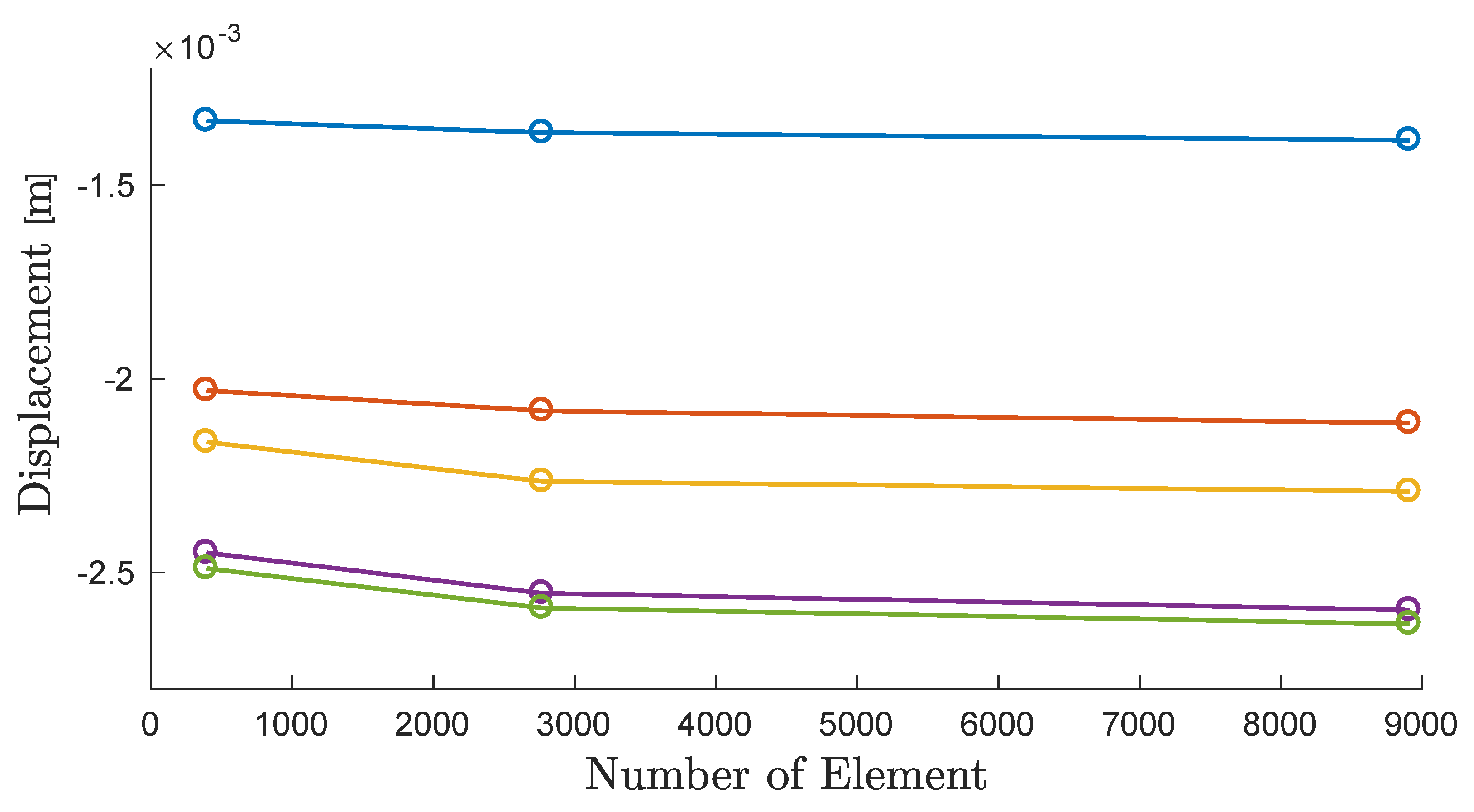
3.2. Mesh Convergence

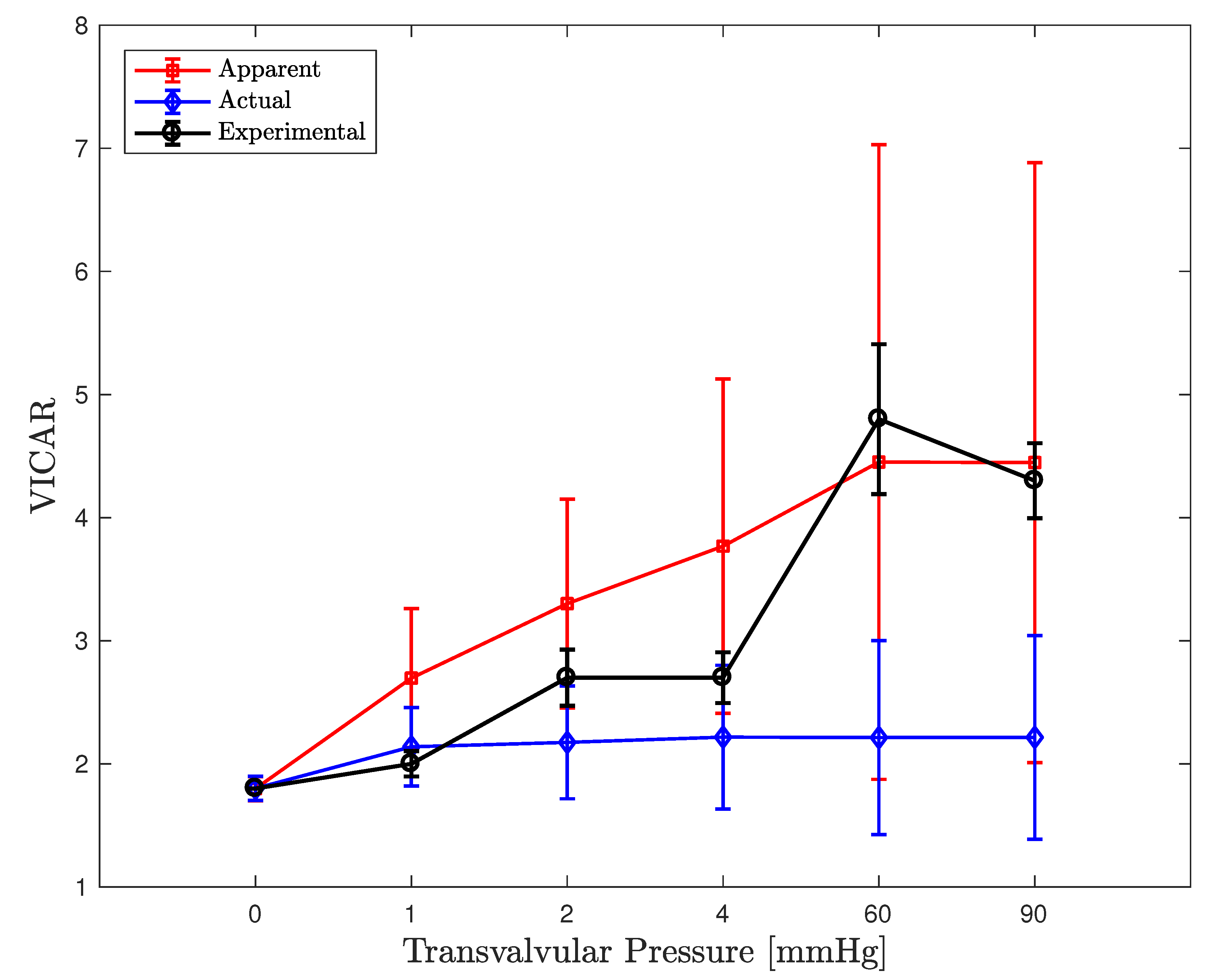
Macroscale: a mesh objectivity study is summarized in Figure 10. The sufficiently converged mesh size, represented by the middle point, was chosen for computational considerations.

Microscale: the convergence of the embedded RVE (Figure 6 right) in the FE${}^2$ procedure is not of interest as it is intentionally downsampled. The postprocessing high-fidelity mesh (Figure 6 left) mesh is relatively straightforward because we impose deformations everywhere in the domain (Taylor boundary conditions). Our quantity of interest is the VICAR, so the mesh must be sufficiently dense such that there is high probability that nodes are close enough to the apexes of the ellipsoid in the (randomized) unstructured tetrahedral mesh generation. We controlled the mesh density with a parameter that enforces a maximum element area on the surface of the ellipsoid, $A_{max}$, in the Delaunay triangulation [42].

3.3. FE${}^2$ Result: Healthy Valve

Simulations were tested on an in-house 32-node cluster, Iron, and run on 60 nodes of the 8109 cluster SAVIO (http://research-it.berkeley.edu/services/high-performance-computing accessed on 1 September 2021). Each simulation ran for approximately 20 h on the latter.

The deformed shapes of the AV leaflet simulated under the five steps of the loading protocol defined in Table 1 can be seen in Figure 11. We computed an average Jacobian in all the elements throughout the loading of $J=det\mathit{F}\approx 1$, within 1.5%, indicating the desired quasi-incompressible behavior.

Valvular interstitial cell aspect ratio (VICAR): the VICAR plots are computed from the RVEs at every Gauss point in the elements along the symmetry plane: a total of $144\times 8=1152$ RVEs. The average was reported, and where shown, error bars represent standard deviation. Note that the authors of the experimental data did not specify whether their error bars represented one standard deviation or one standard error.

Throughout this discussion, a two-tailed t-test was used to test significant differences in means. We used the term significant to indicate that the p-value is $p<0.05$ for the t-test, i.e., the difference in means is statistically significant.

Simulated VICAR ratios for ${\sigma }_{\theta }=5^{\circ }$ and the volume ratio VR = 0.01 were calculated for different transvalvular pressures (see Figure 12). In the figure, the red curve indicates “apparent” VICAR and the blue curve is the actual VIC aspect ratio (see Figure 7 and the corresponding discussion). The black curve is experimental data from [5].

We then examined the effect of varying the parameters ${\sigma }_{\theta }$ and the volume ratio (VR) on the “apparent” VICAR (see Figure 13). We only observed a significant difference in the “apparent” VICAR at ${\sigma }_{\theta }={20}^{\circ }$ vs. ${\sigma }_{\theta }=\{5^{\circ },{10}^{\circ }\}$, with a remarkable decrease in the former. No significant variation was found when varying VR over two orders of magnitude.

We then briefly looked at the initial cusp curvature defined by (19). Figure 14 demonstrates the variation of the VICAR with respect to $y_0$, as a fraction of the size parameter r (e.g., an offset of $10\%\Rightarrow y_0=0.1r$). Significant but small differences are observed throughout. We note that for large values of $y_0$, convergence issues in the FE problem were encountered.

Finally, Figure 15 demonstrates the VICAR in each layer. Significant differences were observed everywhere except between the spongiosa and ventricularis at low pressures. The fibrosa demonstrates a larger VICAR, consistent with experimental findings.

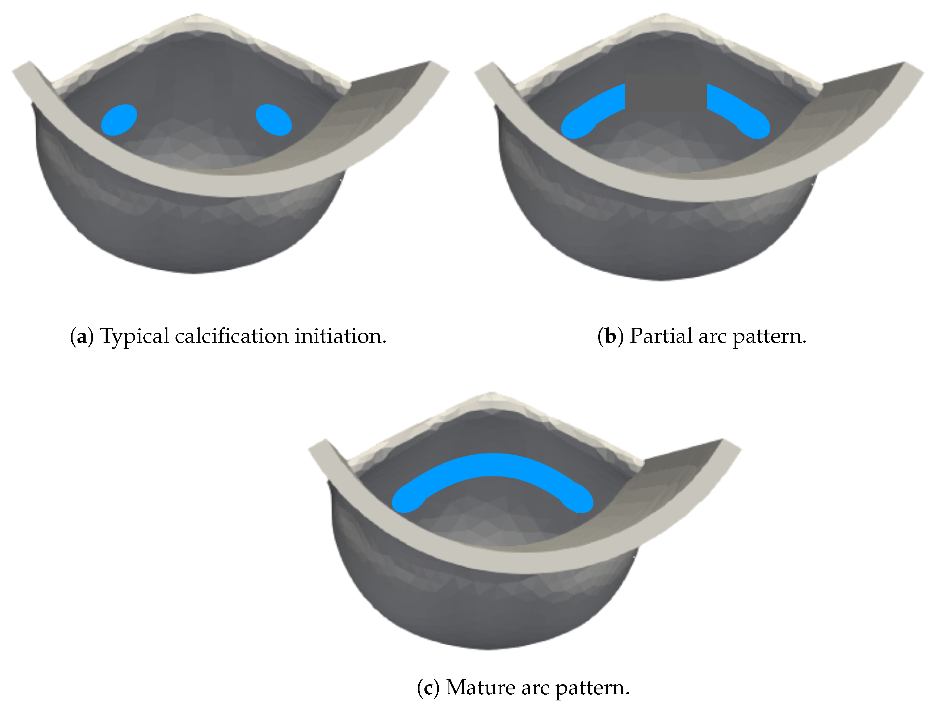
3.4. Calcified Valve: Early-Stage Nodules

Leaflet deformations under five loading conditions as defined under the loading protocol outlined in Table 1 with one calcification nodule pattern are shown in Figure 16. Comparison of these deformation patterns to those presented in Figure 11 show the effect of one early-stage nodule. We maintain quasi-incompressible behavior as in the calcification-free model. The strain component plotted is the 11 Almansi strain in the laboratory Cartesian system and a mapping to the CRT coordinates, via (19), is required to recover the circumferential strain. Note the kinking of deformation in the belly region at high pressures.

Valvular interstitial cell aspect ratio (VICAR): in Figure 17, we see the VIC aspect ratio (VICAR) with the presence of calcified nodules (Figure 8a). Note that the calculation excludes VICs in the calcified regions. The “apparent” VICAR (Figure 17a) in the belly region of the leaflet is slightly smaller than the healthy case (significant only at 60 and 90 mmHg). The actual VICAR is, however, higher (more significant) than the healthy case (Figure 17b).

3.5. Calcified Valve: Partial Arc Pattern

The deformed shape of the calcified AV leaflet was examined at the five steps of the loading protocol outlined in Table 1 (see Figure 18). Comparing the results with those in Figure 11, we can see the result of the partial arc calcification pattern on the leaflet tissue deformation. We maintain quasi-incompressible behavior as in the calcification-free model.

Valvular interstitial cell aspect ratio (VICAR): the effect of partial arc calcification (Figure 8b) can be quantified by examining the VICAR aspect ratios presented in Figure 19. Note that the calculation excludes VICs in the calcified regions. The “apparent” VICAR (Figure 19a) along the belly is slightly smaller than the healthy case (significant only at 60/90 mmHg). The actual VICAR is, however, higher (more significant) than the healthy case (Figure 19b).

3.6. Calcified Valve: Mature Arc Pattern

Finally, the effect of the end-stage calcification on the AV leaflet tissue was examined by comparing the deformed shape at the five steps of the loading protocol outlined in Table 1 (see Figure 11 and Figure 20). Again, we maintained quasi-incompressible behavior as in the calcification-free model.

Valvular interstitial cell aspect ratio (VICAR): in Figure 21, we see the VICAR with the presence of a mature calcified arc pattern (Figure 8c). The “apparent” VICAR (Figure 21a) along the belly is noticeably smaller than the healthy case (significant). The actual VICAR is, unlike the nodules, slightly lower (less significant) than the healthy case (Figure 21b).

4. Discussion

4.1. Healthy Valve

Macroscale model: we designed a set of simulations that mimic the experiments of Huang [4] to validate a multiscale modeling approach for AV tissue, namely the pressurization of a “fixed” valve leaflet loaded from the aortic side. This corresponds to the region in the cardiac cycle between systole and diastole (Figure 2) where the transvalvular pressure is the largest.

These boundary conditions represent in vitro experiments rather than the proper in vivo conditions. They allow us to simulate physiological states in the laboratory. The nature of the fixed boundary conditions, including the “free” coaptation edge, results in a “balloon-inflation”-like response, as seen in Figure 11. The response is consistent with the material response in Figure 9. The low pressure (load) results in the large deformation of the compliant regime. The tissue quickly stiffens and we see only small changes in the deformation for larger increasing loads. Note that we have not pre-stressed the tissue as in [39].

The initial curvature also plays a role in the response of the tissue, and we also encountered convergence issues for variations of the parameters in (19). However, without “patient-specifc” geometry, the best we can hope for is an aggregate consistent result, which we observe in Figure 12.

Representative volume element (RVE): at the heart of our model is the RVE. We first discuss several of the important assumptions we made. Miehe et al. [43] argue that due to the averaging process in homogenization, the details of the RVE do not greatly impact the macroscale problem, something we also observe. To facilitate computational efficiency, we downsampled the RVE mesh and use an auxiliary high-fidelity mesh to extract details in a post-processing step (Figure 6).

Again, for efficiency purposes, we assume Taylor boundary conditions, which results in an overestimation of stiffness response [44]. We also use Taylor boundary conditions in the VICAR post-processing for consistency. Figure 22 illustrates the difference in VICAR with Taylor and Dirichlet boundary conditions. As expected, the Dirichlet VICAR is on average lower. This is a result of only imposing motions on the boundaries and also allowing for a relaxation of the VIC. Note that although the difference is large for the “apparent” VICAR, we did not see a large difference in the actual VICAR.

Finally, we assume the VIC bonds perfectly with the ECM, which is not physiologically accurate (see [45]). Modeling the discrete attachments via focal adhesions of the VIC requires special attention and is left as a limitation of the current study. Note, however, that by explicitly modeling the VICs in the RVE, such an extension is possible within our framework.

VICAR: the aspect ratio being measured in the experiments is that of the nucleus, not the cell. We do not make a distinction between the nucleus and the cell in this analysis, i.e., we neglect the cytoskeleton. This is in line with previous analyses [5,6]. We recommend a more detailed model incorporating this distinction for a future study.

The most notable result above is the large discrepancy between the actual and “apparent” VICAR, as seen in Figure 12. We observe that the (arithmetic) mean “apparent” response is more consistent with the experimental results. We note that there is also large variation in the “apparent” ratio.

The procedure used to determine the “apparent” value, as depicted in Figure 7, is representative of the experiments but not exactly identical. Notwithstanding, the results show that the observed cellular deformation may be significantly different than the true deformation. This is of great importance when developing mechanotransduction models calibrated from experiments.

Figure 12, Figure 13 and Figure 14 show that the “apparent” response is not highly sensitive to the RVE (or macroscale) configuration, and that the largest source of discrepancy between the apparent and actual response comes from the “perspective” used to measure (i.e., the projection of the ellipsoid on the cutting plane). Thus, the orientation of the cutting plane has the greatest impact.

In Figure 13, we observe the “apparent” VICAR closer to the actual VICAR for ${\sigma }_{\theta }={20}^{\circ }$. However, the true distribution of the cell orientation is closer to ${\sigma }_{\theta }\le {10}^{\circ }$, due to the consistency of the “apparent” VICAR with the experiments. The larger ${\sigma }_{\theta }$ represents more variance in the cutting planes’ orientations (i.e., the “perspective”), resulting in the smallest discrepancy between the “apparent” and actual VICAR. In other words, not adequately controlling for the cutting plane orientation (or alternatively, not spanning enough possible cutting plane orientations) can lead to a large discrepancy between the VICAR measured in the lab and the true VICAR.

Finally, Figure 15 shows that the greatest deformation in the tissue occurs in the fibrosa, consistent with previous findings [5,6]. Indeed, the prevalence of calcification in the top layer of the fibrosa, a process driven by circumferential strain in the VIC, is consistent with this [3,18].

4.2. Calcified Valve

Early-stage nodules: although not clear from Figure 16, the average Almansi circumferential strain in the belly region of the leaflet with calcified nodules is on average ∼$20\%$ larger than the healthy leaflet (

Table 3. Average ratio of the circumferential and radial Almansi strains in the belly region seen in a leaflet with a calcific nodule relative to values seen in a healthy leaflet.

Load (mmHg)	1	2	4	60	90
Circumferential Strain Ratio	0.96	1.19	1.32	1.26	1.21
Radial Strain Ratio	$-0.39$	0.14	0.31	0.42	0.41

). Conversely, the radial Almansi strain is on average ∼$17\%$ of the healthy model.

Taking a closer look at the microscale response of the actual VICARs in Figure 17b, we note that the average VIC indeed experiences a larger (significant) aspect ratio than the healthy case. Interestingly, we observe little difference in the “apparent” VICAR in Figure 17a. In fact, we only see a slight (significant) decrease in the VICAR at 60 mmHg.

Note the increased circumferential strain (VICAR) due to the presence of calcified nodules. Previous studies have indicated that the increased circumferential strain results in calcification growth [3,18]. Thus, one would expect that the nodules would grow into more mature patterns with the increased circumferential strain.

Partial arc pattern: the partial arc serves as both a different “mature” pattern example, and as a midway stage between the nodule and the full arc cases. We see a disturbed deformed state via the kink in the belly region, where there is a large discontinuity in stiffness from the calcified region (Figure 18). Indeed, calcified valves exhibit abnormal (and inefficient) dynamics, such as in stenosis or regurgitation. Furthermore, A larger VICAR indicates further progression of the calcification.

Mature arc pattern: it is clear from Figure 20 that the calcified leaflet experiences significantly lower strain. In fact, we see an average ∼$43\%$ reduction in the circumferential Almansi strain, and an inversion of the radial Almansi strain for low (<60 mmHg) pressures. One can argue that the decreased circumferential pattern limits the development of further calcification, resulting in a natural “saturation” of the calcification.

Taking a closer look at the microscale response of the VICs in Figure 21, we note that the average VIC indeed experiences a decreased aspect ratio (i.e., relative to the VIC ellipsoid principal axes), for both the “apparent” (significant) and actual (significant for 1, 2, or 4 mmHg).

4.3. Computational Considerations

As mentioned previously, one full day of computation on 60 nodes of a computational cluster is required for a quasi-static analysis with simplified RVE boundary conditions. This is representative of only one small part of the cardiac cycle. Indeed, more relevant cyclic dynamic problems with more suitable RVE boundary conditions can prove to be challenging. Nevertheless, the method is computationally tractable, and the abundant availability of large computing resources, as of the time of this study, render this issue at most an inconvenience.

4.4. Summary and Outlook for Future Extensions

In this work, we demonstrated the feasibility of using computational homogenization, or FE${}^2$, for modeling the coupled, multiscale behavior of aortic valve (AV) tissue. The natural extension is to model the full aortic valve geometry with the time-resolved dynamics of the AV solid and fluid mechanics. We argue that multiscale modeling is necessary for understanding AV behavior and the method we presented provides a feasible way of achieving a fully coupled multiscale analysis for aortic valves. Furthermore, the RVEs can be used to develop cellular-driven models.

We further utilized the multiscale AV leaflet model to study three calcification topologies as idealized representations of different stages of calcific aortic stenosis progression: early-stage nodules, a partial arc, and a mature arc pattern. In the former, we saw that the presence of the calcification nodules led to a larger circumferential Almansi strain and VIC aspect ratio that presumably drives further calcification growth in a positive-feedback loop manner. Furthermore, we noticed that the “apparent” aspect ratio, as measured by slicing a section of the tissue and observing the 2D aspect ratio of the cell cross-section, did not necessarily exhibit the true aspect ratio.

In the more advanced calcification cases, we observed the disturbed biomechanics of the leaflet which presumably results in stenotic behavior. We observed a lower aspect ratio consistent with a natural “saturation” of the calcification in our full arc calcification computations. Our study, however, was limited to static in vitro loading, to validate it against experiments in the literature. A follow-up study should be performed with dynamic and cyclic loading using an in vivo configuration of the AV leaflet. Furthermore, the extension study should feature stochastic representations of the calcification topology, perhaps via strain-driven growth models [3,18].

References

1. Sacks, M.S.; Liao, J. (Eds.) Advances in Heart Valve Biomechanics: Valvular Physiology, Mechanobiology, and Bioengineering; Springer International Publishing: Cham, Switzerland, 2018. [Google Scholar]
2. Taylor, P.M.; Batten, P.; Brand, N.J.; Thomas, P.S.; Yacoub, M.H. The Cardiac Valve Interstitial Cell. Int. J. Biochem. Cell Biol. 2003, 35, 113–118. [Google Scholar] [CrossRef]
3. Arzani, A.; Mofrad, M.R.K. A Strain-based Finite Element Model for Calcification Progression In Aortic Valves. J. Biomech. 2017, 65, 216–220. [Google Scholar] [CrossRef] [PubMed] [Green Version]
4. Huang, H.Y.S. Micromechanical Simulations of Heart Valve Tissues. Ph.D. Thesis, University of Pittsburgh, Pittsburgh, PA, USA, 2004. [Google Scholar]
5. Huang, H.Y.S.; Liao, J.; Sacks, M.S. In-situ Deformation of the Aortic Valve Interstitial Cell Nucleus Under Diastolic Loading. J. Biomech. Eng. 2007, 129, 880–889. [Google Scholar] [CrossRef] [PubMed] [Green Version]
6. Weinberg, E.J.; Mofrad, M.R.K. Transient, Three-dimensional, Multiscale Simulations of the Human Aortic Valve. Cardiovasc. Eng. 2007, 7, 140–155. [Google Scholar] [CrossRef] [PubMed]
7. Huang, S.; Huang, H.Y.S. Virtual Experiments of Heart Valve Tissues. In Proceedings of the 2012 Annual International Conference of the IEEE Engineering in Medicine and Biology Society, San Diego, CA, USA, 28 August–1 September 2012; pp. 6645–6648. [Google Scholar]
8. Weinberg, E.J.; Mofrad, M.R.K. A Multiscale Computational Comparison of the Bicuspid and Tricuspid Aortic Valves In Relation To Calcific Aortic Stenosis. J. Biomech. 2008, 41, 3482–3487. [Google Scholar] [CrossRef] [PubMed]
9. Weinberg, E.J.; Schoen, F.J.; Mofrad, M.R.K. A Computational Model of Aging and Calcification In the Aortic Heart Valve. PLoS ONE 2009, 4, e5960. [Google Scholar] [CrossRef] [PubMed]
10. Kouznetsova, V.G. Computational Homogenization for the Multi-Scale Analysis of Multi-Phase Materials. Ph.D. Thesis, Eindhoven University of Technology, Eindhoven, The Netherlands, 2002. [Google Scholar]
11. Aikawa, E.; Hutcheson, J.D. Cardiovascular Calcification and Bone Mineralization; Springer Nature: Cham, Switzerland, 2020. [Google Scholar]
12. Thubrikar, M.J. The Aortic Valve; CRC Press: Boca Raton, FL, USA, 1989. [Google Scholar]
13. Ahrens, J.; Geveci, B.; Law, C. Paraview: An End-User Tool for Large-Data Visualization. In Visualization Handbook; Hansen, C.D., Johnson, C.R., Eds.; Butterworth-Heinemann: Burlington, MA, USA, 2005; pp. 717–731. [Google Scholar]
14. Stewart, B.F.; Siscovick, D.; Lind, B.K.; Gardin, J.M.; Gottdiener, J.S.; Smith, V.E.; Kitzman, D.W.; Otto, C.M. Clinical Factors Associated With Calcific Aortic Valve Disease fn1. J. Am. Coll. Cardiol. 1997, 29, 630–634. [Google Scholar] [CrossRef] [Green Version]
15. Mohler, E.R.; Gannon, F.; Reynolds, C.; Zimmerman, R.; Keane, M.G.; Kaplan, F.S. Bone Formation and Inflammation In Cardiac Valves. Circulation 2001, 103, 1522–1528. [Google Scholar] [CrossRef]
16. Rajamannan, N.M.; Subramaniam, M.; Rickard, D.; Stock, S.R.; Donovan, J.; Springett, M.; Orszulak, T.; Fullerton, D.A.; Tajik, A.J.; Bonow, R.O. Human Aortic Valve Calcification Is Associated with an Osteoblast Phenotype. Circulation 2003, 107, 2181–2184. [Google Scholar] [CrossRef]
17. Thubrikar, M.J.; Aouad, J.; Nolan, S.P. Patterns of Calcific Deposits In Operatively Excised Stenotic Or Purely Regurgitant Aortic Valves and Their Relation To Mechanical Stress. Am. J. Cardiol. 1986, 58, 304–308. [Google Scholar] [CrossRef]
18. Halevi, R.; Hamdan, A.; Marom, G.; Mega, M.; Raanani, E.; Haj-Ali, R. Progressive Aortic Valve Calcification: Three-dimensional Visualization and Biomechanical Analysis. J. Biomech. 2015, 48, 489–497. [Google Scholar] [CrossRef]
19. Otto, C.M.; Kuusisto, J.; Reichenbach, D.D.; Gown, A.M.; O’Brien, K.D. Characterization of the early lesion of `degenerative’ valvular aortic stenosis. Histological and immunohistochemical studies. Circulation 1994, 90, 844–853. [Google Scholar] [CrossRef] [Green Version]
20. Weinberg, E.J.; Shahmirzadi, D.; Mofrad, M.R.K. On the Multiscale Modeling of Heart Valve Biomechanics In Health and Disease. Biomech. Model. Mechanobiol. 2010, 9, 373–387. [Google Scholar] [CrossRef] [PubMed]
21. Yip, C.Y.Y.; Simmons, C.A. The Aortic Valve Microenvironment and Its Role In Calcific Aortic Valve Disease. Cardiovasc. Pathol. 2011, 20, 177–182. [Google Scholar] [CrossRef] [PubMed]
22. Ge, L.; Sotiropoulos, F. Direction and Magnitude of Blood Flow Shear Stresses on the Leaflets of Aortic Valves: Is There a Link With Valve Calcification? J. Biomech. Eng. 2010, 132, 014505. [Google Scholar] [CrossRef] [PubMed]
23. Balachandran, K.; Sucosky, P.; Jo, H.; Yoganathan, A.P. Elevated Cyclic Stretch Alters Matrix Remodeling In Aortic Valve Cusps: Implications for Degenerative Aortic Valve Disease. Am. J. Physiol.-Heart Circ. Physiol. 2009, 296, H756–H764. [Google Scholar] [CrossRef] [PubMed]
24. Bouchareb, R.; Boulanger, M.C.; Fournier, D.; Pibarot, P.; Messaddeq, Y.; Mathieu, P. Mechanical Strain Induces the Production of Spheroid Mineralized Microparticles In the Aortic Valve Through a Rhoa/rock-dependent Mechanism. J. Mol. Cell. Cardiol. 2014, 67, 49–59. [Google Scholar] [CrossRef]
25. Merryman, W.D. Mechano-Potential Etiologies of Aortic Valve Disease. J. Biomech. 2010, 43, 87–92. [Google Scholar] [CrossRef] [Green Version]
26. Freeman, R.V.; Otto, C.M. Spectrum of Calcific Aortic Valve Disease: Pathogenesis, Disease Progression, and Treatment Strategies. Circulation 2005, 111, 3316–3326. [Google Scholar] [CrossRef] [PubMed] [Green Version]
27. Yap, C.H.; Saikrishnan, N.; Tamilselvan, G.; Yoganathan, A.P. Experimental Measurement of Dynamic Fluid Shear Stress on the Aortic Surface of the Aortic Valve Leaflet. Biomech. Model. Mechanobiol. 2012, 11, 171–182. [Google Scholar] [CrossRef] [Green Version]
28. Fisher, C.I.; Chen, J.; Merryman, W.D. Calcific Nodule Morphogenesis By Heart Valve Interstitial Cells Is Strain Dependent. Biomech. Model. Mechanobiol. 2013, 12, 5–17. [Google Scholar] [CrossRef] [PubMed]
29. Holzapfel, G.A. Nonlinear Solid Mechanics: A Continuum Approach for Engineering; Wiley: Chichester, UK, 2000. [Google Scholar]
30. Anand, L.; Govindjee, S. Continuum Mechanics of Solids; Oxford University Press: Oxford, UK, 2020. [Google Scholar]
31. Fung, Y.C. Biomechanical Aspects of Growth and Tissue Engineering. In Biomechanics: Motion, Flow, Stress, and Growth; Springer: New York, NY, USA, 1990; pp. 499–546. [Google Scholar]
32. Ball, J.M. Convexity Conditions and Existence Theorems In Nonlinear Elasticity. Arch. Ration. Mech. Anal. 1976, 63, 337–403. [Google Scholar] [CrossRef]
33. Zienkiewicz, O.C.; Taylor, R.L. The Finite Element Method: Solid Mechanics; Butterworth-Heinemann: Oxford, UK, 2000; Volume 2. [Google Scholar]
34. Taylor, R.L.; Govindjee, S. FEAP—Finite Element Analysis Program; University of California: Berkeley, CA, USA, 2020. [Google Scholar]
35. Haj-Ali, R.; Marom, G.; Zekry, S.B.; Rosenfeld, M.; Raanani, E. A General Three-dimensional Parametric Geometry of the Native Aortic Valve and Root for Biomechanical Modeling. J. Biomech. 2012, 45, 2392–2397. [Google Scholar] [CrossRef]
36. Stella, J.A.; Sacks, M.S. On the Biaxial Mechanical Properties of the Layers of the Aortic Valve Leaflet. J. Biomech. Eng. 2007, 129, 757–766. [Google Scholar] [CrossRef] [PubMed]
37. Buchanan, R.M.; Sacks, M.S. Interlayer Micromechanics of the Aortic Heart Valve Leaflet. Biomech. Model. Mechanobiol. 2014, 13, 813–826. [Google Scholar] [CrossRef] [PubMed] [Green Version]
38. Sacks, M.S.; Yoganathan, A.P. Heart valve function: A Biomechanical Perspective. Philos. Trans. R. Soc. B Biol. Sci. 2007, 362, 1369–1391. [Google Scholar] [CrossRef] [PubMed] [Green Version]
39. Bakhaty, A.A.; Govindjee, S.; Mofrad, M.R.K. Consistent trilayer biomechanical modeling of aortic valve leaflet tissue. J. Biomech. 2017, 61, 1–10. [Google Scholar] [CrossRef] [PubMed] [Green Version]
40. Fang, Q.; Boas, D. Tetrahedral mesh generation from volumetric binary and gray-scale images. In Proceedings of the 2009 IEEE International Symposium on Biomedical Imaging: From Nano to Macro, Boston, MA, USA, 28 June–1 July 2009; pp. 1142–1145. [Google Scholar]
41. Rho, J.Y.; Hobatho, M.C.; Ashman, R.B. Relations of Mechanical Properties To Density and CT Numbers In Human Bone. Med. Eng. Phys. 1995, 17, 347–355. [Google Scholar] [CrossRef]
42. Weatherill, N.P.; Hassan, O. Efficient Three-dimensional Delaunay Triangulation With Automatic Point Creation and Imposed Boundary Constraints. Int. J. Numer. Methods Eng. 1994, 37, 2005–2039. [Google Scholar] [CrossRef]
43. Miehe, C.; Schröder, J.; Schotte, J. Computational Homogenization Analysis In Finite Plasticity Simulation of Texture Development In Polycrystalline Materials. Comput. Methods Appl. Mech. Eng. 1999, 171, 387–418. [Google Scholar] [CrossRef]
44. Li, S.; Wang, G. Introduction to Micromechanics and Nanomechanics; World Scientific Publishing Company: Singapore, 2008. [Google Scholar]
45. Mofrad, M.R.K.; Kamm, R.D. Cellular Mechanotransduction: Diverse Perspectives from Molecules to Tissues; Cambridge University Press: Cambridge, UK, 2014. [Google Scholar]
Figure 1. One-sixth of a symmetric idealized aortic valve geometry, as obtained from Weinberg and Mofrad [6]. The leaflet is highlighted. The one-sixth geometry with symmetry planes is used in our models for computational efficiency. Rendering generated with ParaView [13].
Applsci 11 08332 g001
Figure 2. Aortic valve cardiac cycle pressures, as adapted from [12]. The figure shows the ventricular and aortic pressures during systole and diastole phases in three consecutive cardiac cycles.
Applsci 11 08332 g002
Figure 3. Prevalent calcification patterns on the aortic valve. Note that calcification is typically found on the aortic side of the leaflet, as shown in blue [17,18].
Applsci 11 08332 g003
Figure 4. Computational homogenization, i.e., FE 2 . The macro problem passes the deformation gradient F M to the RVE (micro problem), where (1) is solved. The homogenized stress and tangent (as given by (15) and (18)) are then computed and passed up to the macro problem. The process is typically iterated as in (7). This graphic was adapted from Kouznetsova [10].
Applsci 11 08332 g004
Figure 5. Macroscale AV leaflet (symmetric) mesh generated with a custom algorithm and FEAP built-in tools. The r and c directions represent a curvilinear set of coordinates in the surface of the leaflet and t is the coordinate orthogonal to the surface of the leaflet. Paraview was used for visualization [13].
Applsci 11 08332 g005
Figure 6. Right: Low-fidelity RVE mesh used for FE 2 computation; Left: High-fidelity RVE mesh used for post-processing calculation. Both meshes enforce the same volume ratio. Meshes generated and visualized with Iso2mesh [40].
Applsci 11 08332 g006
Figure 7. Visualization [40] of the VICAR measurement. Blue circles indicate the actual VICAR while red circles indicate the “apparent” VICAR as measured via the projection of the ellipsoidal cell on the cutting plane convecting with the deformation.
Applsci 11 08332 g007
Figure 8. Macroscale leaflet meshes with calcified regions highlighted in a teal.
Applsci 11 08332 g008
Figure 9. Equibiaxial membrane stress vs. stretch for RVE material (colored: red is circumferential and blue is radial) and experimental data (black); equibiaxial specimens are extracted from leaflets with radial and circumferential directions as indicated in Figure 5 and detailed in [4]. See [39] for details regarding the fitting of the experiments.
Applsci 11 08332 g009
Figure 10. Convergence study for the macroscale mesh. Each curve represents displacements (in the belly region of the leaflet) at the load steps in Table 1. The mesh size represented by the middle point was chosen for computational considerations.
Applsci 11 08332 g010
Figure 11. Leaflet deformation under the load protocol defined in Table 1. Contours are the 11 Almansi strain component (non-dimensional) in the global laboratory frame.
Applsci 11 08332 g011
Figure 12. VICAR result as an average of 1156 RVEs measured along the radial direction in the center of the leaflet. One standard deviation’s error bars are shown. Red curve indicates “apparent” VIC aspect ratio as measured a la Section 2.2.2 and a blue curve is the actual VIC aspect ratio. The black curve is the experimental data from Huang [5] with undefined error bars.
Applsci 11 08332 g012
Figure 13. The effect of the VIC orientation and size on the “apparent” aspect ratio. We note only a significant difference for 60 and 90 mmHg with the standard deviation of the angle from the VIC: (a) volume ratio (VR) fixed, varying standard deviation of angle (σθ); and (b) standard deviation of angle (σθ) fixed, varying volume ratio (VR).
Applsci 11 08332 g013
Figure 14. The effect of the initial cusp curvature on the VICAR. “Offset” y 0 viz. (19) is reported as a fraction of the size parameter r (e.g., an offset of 10 % y 0 = 0.1 r ). Significant but small differences are observed throughout.
Applsci 11 08332 g014
Figure 15. VICAR as measured in each of the three layers. Significant differences are observed everywhere except at low pressures between the spongiosa and ventricularis.
Applsci 11 08332 g015
Figure 16. Leaflet deformation under load defined in Table 1 with the nodule pattern. The strain plotted is the 11 component of the Almansi strain (non-dimensional) in the laboratory Cartesian system and not the circumferential strain.
Applsci 11 08332 g016
Figure 17. VICAR for early stage calcified nodules. The error bars represent one standard deviation.
Applsci 11 08332 g017
Figure 18. Leaflet deformation under loading defined in Table 1 with the partial arc pattern. Note the calcified regions on the surface. The strain plotted is the 11 component of the Almansi strain (non-dimensional) in the laboratory Cartesian system and not the circumferential strain.
Applsci 11 08332 g018
Figure 19. VICAR for partial arc pattern. The error bars represent one standard deviation.
Applsci 11 08332 g019
Figure 20. Leaflet deformation under load defined in Table 1 with the arc pattern. Note the calcified regions on the surface. The strain plotted is the 11 component of the Almansi strain (non-dimensional) in the laboratory Cartesian system and not the circumferential strain.
Applsci 11 08332 g020
Figure 21. VICAR for mature arc pattern. The error bars represent one standard deviation.
Applsci 11 08332 g021
Figure 22. Effect of RVE boundary conditions on VICAR response. Taylor boundary conditions impose motion everywhere in the domain and Dirichlet boundary conditions only impose motion on the boundary.
Applsci 11 08332 g022