Parallel Makespan Calculation for Flow Shop Scheduling Problem with Minimal and Maximal Idle Time

Abstract

In this paper, a flow shop scheduling problem with minimal and maximal machine idle time with the goal of minimizing makespan is considered. The mathematical model of the problem is presented. A generalization of the prefix sum, called the job shift scan, for computing required shifts for overlapping jobs is proposed. A work-efficient algorithm for computing the job shift scan in parallel for the PRAM model with n processors is proposed and its time complexity of $O(logn)$ is proven. Then, an algorithm for computing the makespan in time $O(mlogn)$ in parallel using the prefix sum and job shift scan is proposed. Computer experiments on GPU were conducted using the CUDA platform. The results indicate multi-thread GPU vs. single-thread GPU speedups of up to 350 and 1000 for job shift scan and makespan calculation algorithms, respectively. Multi-thread GPU vs. single-thread CPU speedups up to 4.5 and 14.7, respectively, were observed as well. The experiments on the Taillard-based problem instances using a simulated annealing solving method and employing the parallel makespan calculation show that the method is able to perform many more iterations in the given time limit and obtain better results than the non-parallel version.

1. Introduction

For several decades, scheduling and job scheduling have received constant attention from both researchers and practitioners from across the world. Such a level of interest is justified by the broad applications of scheduling which go from production planning and manufacturing [1,2], construction [3], cloud computing [4,5], transportation [6], education [7], healthcare [8] to CPUs [9], Internet of Things [10] and sensor networks [11]. Moreover, many scheduling problems are NP-hard, increasing the importance of developing faster and more efficient solving methods for scheduling problems with real-life instance sizes.

In the modern day, the approach to scheduling problems has somewhat changed. In order to better model real-life situations, more specific problem variants with additional constraints are considered. Such constraints may include, for example, transport times [12], setups [13], limited buffers [14] or idle times [15]. As a result, state-of-the-art solving methods often have to employ problem-specific properties to be efficient. Furthermore, due to ever-growing markets and the emergence of Big Data, larger and larger problems are being considered [16,17], which is especially true for cloud scheduling [18,19].

Finally, in recent years, there has been significant growth in the field of parallel and distributed computing. This is due to technologies such as Nvidia’s compute unified device architecture (CUDA) and message passing interface (MPI) as well as developments in parallel devices such as general-purpose computing on graphics processing units (GPGPU) and manycore processors. As a result, parallel computing has become one of the main ways of increasing the effectiveness and reducing the running time of solving methods for scheduling problems [20,21]. This is especially important for reducing the complexity of computing the goal function, which is often the dominant factor in the running time of the solving method [22].

In this paper, a permutation flow shop scheduling problem with makespan criterion and minimal and maximal machine idle time (FSSP-MMI) is considered. A similar, non-permutation variant was previously considered in [23]. FSSP-MMI is a variant of the well-known permutation flow shop scheduling problem (FSSP) [24]. The problem can be used to model some practical processes, e.g., the concreting process (which was described in [23]). Moreover, this problem is also a generalization of several other variants, including: (a) no-idle; (b) minimal idle time; (c) maximal idle time; and (d) classic FSSP. The aim of the paper was to propose a novel parallel computing technique for the faster computation of the goal function for FSSP-MMI and to develop a solving method that is: (1) capable of solving large-size FSSP-MMI problems in reasonable time; and (2) working fast enough for small- and medium-sized FSSP-MMI problems to be applicable as a local-search subroutine in larger algorithms. A parallel algorithm for FSSP-MMI was previously proposed [25], but it required massive numbers of processors, even for small problems. We aimed to rectify this drawback. It should also be noted that while it is intended for FSSP-MMI, the parallel technique will also be applicable for the variants (a)–(d) mentioned above, and with some modifications, for some other variants (e.g., setup times).

As such, the main contributions of this paper can be summarized as follows:

• A job shift scan operation, based on prefix sums, for correcting overlapping jobs and applicable to a large class of scheduling problems, is proposed and proven;
• A work-efficient parallel algorithm for determining the job shift scan in logarithmic time with regard to the number of jobs is proposed;
• A parallel method for the quick calculation of the goal function (makespan) for FSSP-MMI in time $O(mlogn)$ instead of $O\left(mn\right)$ is proposed;
• A simulated annealing metaheuristic solving method, with a parallel makespan calculation for FSSP-MMI, is implemented using the CUDA platform;
• Computer experiments indicate that the proposed solving method is able to obtain better makespans in the same time as its sequential counterpart for large problems.

The rest of the paper is structured as follows. Section 2 contains the literature overview. Section 3 describes the considered scheduling problem. Section 4 contains a short explanation of prefix sums and its parallel computation algorithm. Section 5 describes an extension of the prefix sums for the correction of overlapping jobs and its parallel computation algorithm. In Section 6, a parallel method for a quick calculation of the makespan for the considered problem is proposed. Section 7 describes the proposed metaheuristic solving method. Section 8 contains the computer experiments using the developed solving method. Finally, Section 9 contains the conclusions and future work. Moreover,

Table 1. Summary of notation.

Symbol	Meaning
$\mathcal{J}$, $\mathcal{M}$	Set of jobs, set of machines
n, m	Number of jobs, number of machines
$p_i^a$	Processing time of job i on machine a
$r_a$	Minimal allowed idle time on machine a
$d_a$	Maximal allowed idle time on machine a
$\pi$	Processing order of jobs (solution)
$\pi \left(i\right)$	Job processed as i-th in solution $\pi$
${\pi }^{\prime }$	A neighbor solution of solution $\pi$
${\pi }^{\ast }$	Optimal solution or best-known solution
${\rho }_i^a$	Shorthand for $p_{\pi \left(i\right)}^a$ (solution-adjusted processing time)
$S_i^a$	Starting time of job $\pi \left(i\right)$ on machine a
$C_i^a$	Completion time of job $\pi \left(i\right)$ on machine a
$C_{\max }\left(\pi \right)$	Makespan for solution $\pi$
⊕	Binary operator of the job shift scan
t, E	Current temperature and epoch (solving method parameters)
$T_P$, $T_G$, $T_C$	Running time of solving method variants P, G and C

contains the overview of the notation used throughout the paper.

2. Literature Overview

This section provides a literature overview, focused on two topics: (1) the various additional constraints encountered in FSSP and similar scheduling problems; and (2) the use of parallel computing techniques in solving scheduling problems.

2.1. Problem Constraints

Additional problem constraints are common for scheduling problems. The focus will be on problem constraints that include additional dependencies between the starting or completion times of jobs. First, some authors consider a constraint that forbids starting of a job on any machine before a designated time. Such a constraint is referred to as “ready times”, “release times” or “arrival times” [26,27]. Ready times are common constraints for scheduling on parallel machines [28] and online scheduling [19]. Conversely, the time by which the entire job is expected to be finished, prevalent in construction and civil engineering projects, is commonly called the “due date” or “deadline” [29,30,31].

The next class of constraints are dependencies between the completion of a job on one machine and the starting time of the same job on the next machine, commonly called “wait times”. Two sub-variants are “no-wait”, where the starting time on the next machine is the same as the completion time on the previous machine [32,33,34,35] and “limited wait”, where there is a maximal allowed time before completion and starting on the next machine [27,36]. Some papers also consider both minimal and maximal wait times, sometimes referred to as “time lag” [37,38]. Another type of constraint is the time required to move the job to the next machine, called the “transportation time” [12,39]. It is often used with certain types of manufacturing systems, e.g., ones employing automated guided vehicles (AGVs).

Another group of constraints are dependencies between the completion time of a job on some machine and the starting time of the next job on the same machine. Some very common examples are “setups” or “changeovers”. Setups usually represent the time needed to change the setting of the machine and let it cool down or load the next item. In the simplest form, the setup time depends only on the job that follows it. Such a setup can simply be modeled by extending the processing time of the job. However, it is more common to consider sequence-dependent setup times (SDSTs), where the setup time is dependent on the duration of both the next and previous job [12,13,40].

In general, the time between the processing of subsequent jobs on the same machine is called “idle time”. Similarly to wait times, several sub-variants of this constraint exist. The “no-idle” variant [41,42,43] allows for the maximization of machine utility. This can be useful when the machine cannot be turned off readily or without additional costs. It should also be noted that, while it is rare, it is possible to apply both no-wait and no-idle constraints at the same time [44]. Another type is “minimal idle”—though in practice this is modeled similarly to setups. Similarly, a “limited idle” or “maximal idle” time can be imposed as well [15]. Finally, both the minimal and maximal idle time constraints can be enforced at the same time. This can be used to model some time-sensitive processes in construction, for example, the concreting process [23].

2.2. Parallel Computing

A significant number of approaches in the literature have been dedicated to employing parallel computing techniques to help solving scheduling problems. These approaches vary due to different parallel devices (multicore CPUs versus GPGPUs), parallelization levels (fine- versus coarse-grained), solving methods (population-based versus single-trajectory) and dependency on the problem (mathematically proven problem-specific properties versus run-of-the-mill parallelization). Below is an overview of the recent papers dedicated to this topic, meant to present the diversity of approaches and to highlight the results.

The calculation of the goal function is often the most costly part of solving methods, constituting over 90% of their running time in many cases, as shown in [45]. Thus, considerable effort went into reducing this time. For example, in the mentioned paper, a CUDA-based algorithm was proposed for FSSP with both makespan and total flowtime criteria. The speedup for the resulting tabu search (TS) method was nearly 90 in some cases. A similar approach of fine-grained parallelization for FSSP, suitable for use with GPGPU devices, was shown in [22].

In another paper [46], a method for reducing the computational complexity of calculating the goal function for FSSP with makespan and total flowtime criterion from $O\left(nm\right)$ to $O(n+m)$ was proven. Interestingly, MMX/SSE instructions from the CPUs instruction set were used, making this approach very fine-grained. This allowed to obtain considerably speedup, achievable in any modern PC without the need of multicore processors or specialized GPGPU devices. A similar low-level approach was used in [47] to solve bi-criteria FSSP with simulated annealing (SA). Usually, single-trajectory methods such as SA are harder to parallelize. However, on average, SA rejects several random neighbors before accepting one. Thus, it is more efficient to generate several random neighbors in parallel using MMX/SSE instructions. This reduced the running time of the method, allowing it to obtain better multi-criteria solutions (Pareto fronts). In another paper [25], it was shown that it was possible to compute the goal function for non-permutation FSSP with time couplings in time $O\left({log}^2\left(nm\right)\right)$ instead of $O\left(nm\right)$. Unfortunately, the method requires a very large number of processors, even for small problem sizes. Finally, in paper [48], parallel computing was used to solve the cyclic job shop scheduling problem (JSSP) with the goal of minimizing the cycle time. With the use of the Intel Xeon Phi manycore coprocessor, the authors achieved a speedup of up to 35 times that of the sequential algorithm.

Aside from goal function calculation, other approaches to parallel computing in scheduling problems exist. For example, in paper [49], a very coarse-grained technique was used to enhance the well-known TSAB algorithm for JSSP. While deterministic, TSAB requires several parameters to be calibrated and those values vary for different problem instances. By running many parallel copies of TSAB with different parameters, significantly better results were obtained compared to a single TSAB run without any changes in the underlying algorithm. In another paper [50], genetic algorithm (GA) and ant colony optimization (ACO) were combined and run in parallel to solve multi-criteria JSSP. The combined GACO algorithm obtained better Pareto fronts than either algorithm could separately. However, the need to synchronize both sub-algorithms and update the Pareto set limited the observed speedup. A different result was obtained in work [21], where parallel computing allowed to obtain superlinear speedup for FSSP with the total flowtime criterion. An interesting example is paper [51], where the main memetic algorithm for the FSP is augmented by a local-search procedure. This procedure is required to finish quickly and is thus executed in parallel on a GPGPU device.

GPGPU devices are often used due to the high number of parallel cores they provide, especially when multiple such devices are used together as a part of a computer cluster. However, GPGPUs have a different memory and thread organization compared to CPUs, requiring care in order for the parallel algorithms to be effective. For example, in paper [52], a GPGPU technique for reducing the number of memory accesses was proposed. The technique was then applied to a TS method to solve the FSSP. The results showed speedups of up to 140. As another approach, the authors of paper [53] proposed a modified GA method with islands and a lower–higher structure. This duality was designed to match and take advantage of the lower (block of threads) and higher (grid of blocks) organization scheme of GPGPUs. The obtained results proved competitive quality with reduced running time when compared with a reference method. Similar results were obtained in paper [54], where a parallel GA method for an energy-efficient dynamic flexible FSSP was proposed, reducing the running time up to 25 times. An interesting example was shown in paper [20], where many GPGPU devices, for a total of 2 million CUDA cores, and the branch-and-bound method were used to solve 11 previously unsolved Taillard instances to optimality and update bounds on a further eight instances. For the largest instances, 64 years’ worth of CPU time was computed in just 13 h.

Finally, while authors usually focus on one type of parallel device—GPGPUs or multicore/manycore processors—there are exceptions. This was the case in paper [55], where the authors considered a GA method that employed a hybrid GPGPU + CPU + SSE configuration and used it to solve a large-size flexible FSSP. Aside from the speedups and improved quality, the results indicated the importance of SSE vectorization. For a further reading on the use of parallel computing methods in scheduling, please refer to [56].

3. Problem Formulation

A manufacturing system with n jobs from the set ${\mathcal{J}}^{=}\{1,2,\cdots ,n\}$ and m machines from the set $\mathcal{M}=\{1,2,\cdots ,m\}$ is considered. Each job i has to be processed on all machines with $p_i^a>0$ denoting the processing time of job i on machine a. Moreover, for each machine a, the values $r_a\ge 0$ and $d_a\ge r_a$ denote the minimal and maximal idle time, respectively. Thus, after completing the processing of one job and before starting the processing of the next one, machine a has to wait for time t, such that $t\ge r_a$ and $t\le d_a$.

Each job has to be processed on machines in the order of increasing machine number: $1\to 2\to \cdots \to m$. This order is fixed and represents the technological process. On the other hand, the order of the processing of jobs is the same for each machine and is a decision variable of the problem. This order is described by n-element tuple $\pi$ where the element $\pi \left(i\right)$ denotes the job that is processed as i-th. Henceforth, $\pi$ will be called the solution. Furthermore, a few additional constraints exist. Namely, at any given time, a job can be processed by at most one machine. Similarly, at any given time, a machine can process at most one job. Finally, the processing of jobs cannot be interrupted.

From the solution $\pi$, one can construct a schedule as the sequence S:

$$S=(S^1,S^2,\cdots ,S^m),$$

(1)

where $S^a$ is in turn another sequence describing the starting time of jobs on machine a:

$$S^a=(S_1^a,S_2^a,\cdots ,S_n^a).$$

(2)

Thus, $S_i^a$ is the starting time of job $\pi \left(i\right)$ on machine a. Similarly, one can define sequence C of the job completion times, such that $C_i^a$ is the completion time of job $\pi \left(i\right)$ on machine a. For the simplicity of the notation value, ${\rho }_i^a$ will be used as shorthand for $p_{\pi \left(i\right)}^a$. As such, the schedule S is feasible if and only if all the following constraints are met:

$$\begin{array}{cc}\hfill \forall a\in \mathcal{M}\forall i\in \mathcal{J}& C_i^a=S_i^a+{\rho }_i^a,\hfill \end{array}$$

(3)

$$\begin{array}{cc}\hfill \forall a\in \mathcal{M}\setminus \left\{1\right\}\forall i\in \mathcal{J}& S_i^a\ge C_i^{a-1},\hfill \end{array}$$

(4)

$$\begin{array}{cc}\hfill \forall a\in \mathcal{M}\forall i\in \mathcal{J}\setminus \left\{1\right\}& r_a\le S_i^a-C_{i-1}^a\le d_a.\hfill \end{array}$$

(5)

Constraint (3) ensures that the processing of jobs is not interrupted. Due to constraint (4), a job is completed on machine $a-1$ before it starts processing on machine a (enforcing compliance with the technological process). Finally, constraint (5) ensures that jobs on machine a are processed in the order given by solution $\pi$ and that the minimum and maximum idle times $r_a$ and $d_a$ on machine a are respected. It should be noted that due to (3), both S and C can unambiguously describe the schedule.

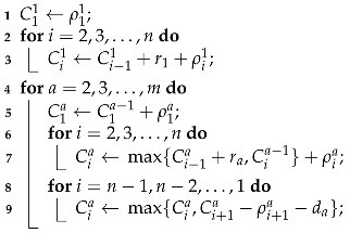
A possible method of constructing schedule C from solution $\pi$ is described by Algorithm 1. The method is nearly identical to the one shown for the non-permutation variant of the problem in [23]. In line 1, the completion time for processing job $\pi \left(1\right)$ on machine 1 is set, since that job has no constraints. In lines 2–3, the completion times for the remaining jobs on machine 1 in order from $\pi \left(2\right)$ to $\pi \left(n\right)$ are set. Since there is no previous machine and $d_a\ge r_a$, only the constraint (3) and the left side of constraint (5) have to be met. In lines 4–9, the completion times on the remaining machines are calculated, always finishing the calculations on machine $a-1$ before moving to machine a. Lines 5–7 are similar to lines 1–3, except the completion time of the same job from the previous machine (terms $C_1^{a-1}$ and $C_i^{a-1}$) is also taken into account. After this, all constraints on machine a are met except for the right side of constraint (5). This is corrected by lines 8–9, where the completion time $C_i^a$ is increased appropriately if the difference between $C_i^a$ and $S_{i+1}^a$ is more than $d_a$. It should be noted that, this time, the jobs are processed from $\pi (n-1)$ down to $\pi \left(1\right)$, so the jobs completing later are corrected first. Due to this, there is a guarantee that each job will have to be shifted at most once. The resulting schedule is always feasible. Moreover, the schedule is always left-shifted as any decrease in any of the completion times would either violate one of the constraints (3)–(5) or would not correspond to the solution $\pi$. It should also be noted that Algorithm 1 is also sequential and that its running time is $O\left(nm\right)$ using a single processor.

Algorithm 1 Constructing left-shifted schedule C from the solution $\pi$

Finally, let $C_{\max }\left(\pi \right)$ be the completion time of the job that completes as last in the schedule described by solution $\pi$, meaning that:

$$C_{\max }\left(\pi \right)=\underset{j\in \mathcal{J}}{max}{C}_j^m=C_n^m.$$

(6)

The value $C_{\max }\left(\pi \right)$ is commonly referred to as makespan. The goal of optimization is to find a solution ${\pi }^{*}$ that minimizes the makespan, meaning that:

$$C_{\max }\left({\pi }^{\ast }\right)=\underset{\pi \in \prod }{min}{C}_{\max }\left(\pi \right),$$

(7)

where $\prod$ is the set of all possible solutions. Solution ${\pi }^{\ast }$ is called the optimal solution.

To summarize, the mathematical model of the problem can be stated as follows:

$$\begin{array}{}\mathrm{(8)}\hfill minimize& C_{\max }\left(\pi \right),\hfill & \mathrm{(9)}\hfill subjectto& C_i^a-S_i^a-{\rho }_i^a=0\hfill & \hfill \forall a\in \mathcal{M}\forall i\in \mathcal{J},\mathrm{(10)}\hfill & C_i^{a-1}-S_i^a\le 0\hfill & \hfill \forall a\in \mathcal{M}\setminus \left\{1\right\}\forall i\in \mathcal{J},\mathrm{(11)}\hfill & S_i^a-C_{i-1}^a\ge r_a\hfill & \hfill \forall a\in \mathcal{M}\forall i\in \mathcal{J}\setminus \left\{1\right\},\mathrm{(12)}\hfill & S_i^a-C_{i-1}^a\le d_a\hfill & \hfill \forall a\in \mathcal{M}\forall i\in \mathcal{J}\setminus \left\{1\right\},\mathrm{(13)}\hfill and& \pi \in \prod ,\hfill & \end{array}$$

where values S, C and $\rho$ are calculated from $\pi$, as shown in Algorithm 1.

4. Parallel Prefix Sum

This section briefly describes the concept of a prefix sum and the algorithm for its parallel computation. Prefix sums will be used both directly as part of the final algorithm as well as indirectly as a basis for the construction of a custom scan-like operation. It should be noted that all information in this section is well known in the literature.

Let $x=(x_1,x_2,\cdots ,x_n)$ be a sequence of n numbers. Then, the inclusive prefix sum of x is defined as sequence of n numbers $y=(y_1,y_2,\cdots ,y_n)$ such that:

$$y_i=\sum _{j=1}^i{x}_i.$$

(14)

In other words, $y_i$ holds the sum of all elements of x up to the i-th element and including it. Similarly, the exclusive prefix sum is defined as the sequence $y^{\prime }=(y_1^{\prime },y_2^{\prime },\cdots ,y_n^{\prime })$ such that:

$$\begin{array}{cc}\hfill y_1^{\prime }& =0,\hfill \end{array}$$

(15)

$$\begin{array}{cc}\hfill y_i^{\prime }& =\sum _{j=1}^{i-1}{x}_{i}i>1.\hfill \end{array}$$

(16)

Thus, $y_i^{\prime }$ holds the sum of all elements up to the i-th but without including it. It should also be noted that transforming between y and $y^{\prime }$ is easy as

$$y_i=y_i^{\prime }+x_i,$$

(17)

or alternatively:

$$\begin{array}{cc}\hfill y_i& =y_{i+1}^{\prime },i<n\hfill \end{array}$$

(18)

$$\begin{array}{cc}\hfill y_n& =y_n^{\prime }+x_n.\hfill \end{array}$$

(19)

The concept of prefix sums has many applications, as pointed out by Blelloch [57]. Various authors have applied them to robotics [58], text pattern matching [59] and k-means clustering [60]—among other applications.

Let us discuss the computation complexity of determining prefix sums y and $y^{\prime }$ for a sequence x of n elements. On a single processor, computing either sum requires performing n additions for a total run time of $O\left(n\right)$ using the simple recursive formula:

$$\begin{array}{cc}\hfill y_1& =x_1,\hfill \end{array}$$

(20)

$$\begin{array}{cc}\hfill y_i& =y_{i-1}+x_{i}i>1\hfill \end{array}$$

(21)

For parallel algorithms, Hillis and Steele [61] proposed an algorithm that runs on PRAM with n processors in time $O(logn)$. Unfortunately, this algorithm is not work-efficient as the total number of addition operations performed is $O(nlogn)$.

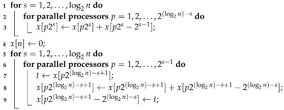
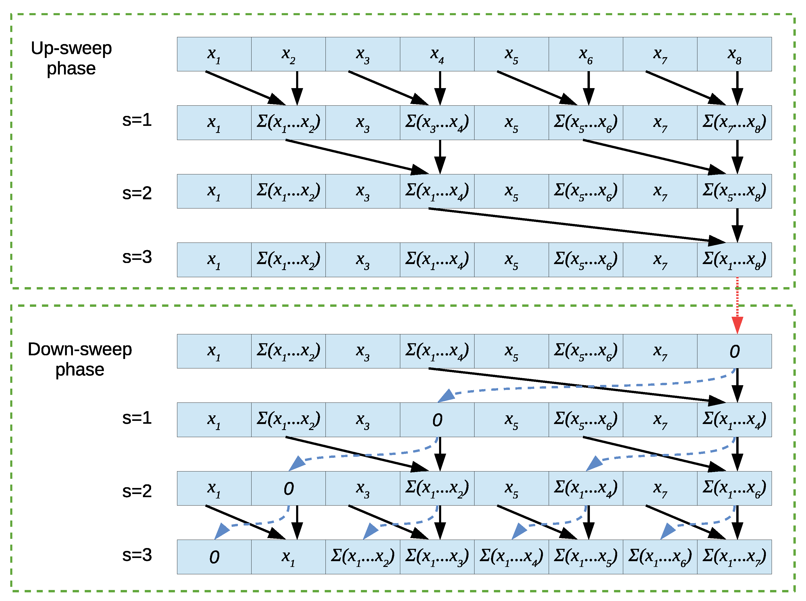
A work-efficient algorithm exists, as was shown by Blelloch [57], and its pseudocode is presented in Algorithm 2. The algorithm works in-place and consists of two major phases: up-sweep and down-sweep. The phases are based on the leaves-to-root and root-to-leaves traversal of binary trees, respectively. The example of how the algorithm works at each step is shown in Figure 1 for $n=8$. Black arrow pairs indicate addition, blue dashed arrows indicate copying and the dotted red arrow indicates the zeroing of the last element.

Algorithm 2 Work-efficient exclusive parallel prefix sum computation

Lines 1–3 correspond to the up-sweep phase. This phase has $logn$ steps. In each step, a number of processors compute partial sums. At the end of this phase, the element $x\left[n\right]$ holds the sum of all elements. Then, in line 4, we zero that element and start the down-sweep phases which happen in lines 5–9. This phase is more complex. At each step, first the value of the “right” element is stored in the temporary variable t (which is a separate private variable for each processor). This corresponds to the start of the blue arrow. Then, a regular addition of the “left” and “right” element is performed and the result is stored in the “right” element. Finally, the blue copying operation is completed by putting the stored value t in the “left” element. The entire algorithm performs $2(n-1)$ additions, $n-1$ copy operations and one zeroing of an element. It thus runs in time $O(logn)$ on PRAM with n processors and performs $O\left(n\right)$ additions. One issue is that the base form of the algorithm assumes that n is a power of 2. However, this can be remedied by running the algorithm for size $k=2^{\lceil logn\rceil }$ and then either skipping operations that modify elements above element n or discarding the part of the output beyond element n. Let us also note that although Algorithm 2 computes the exclusive prefix sum only, Equations (17)–(19) can be used to quickly transform this result into an inclusive prefix sum.

5. Parallel Job Shift Scan

The concept of prefix sums is based on the addition operator +. However, it was shown before (e.g., by Bleboch [57]) that the idea can be generalized for a larger class of associative binary operations, for example, the multiplication or maximum. Such a prefix sum generalization is usually called a “scan”. One such scan operation that pertains to scheduling problems will be proposed in this section.

As an example, a schedule for some machine a in the FSSP with $n=8$ jobs will be considered. Assume the starting and completion times for jobs on that machine have been set as follows:

$$\begin{array}{cc}\hfill S^a& =(0,1,5,13,14,16,25,28),\hfill \end{array}$$

(22)

$$\begin{array}{cc}\hfill C^a& =(4,6,7,16,19,22,29,31).\hfill \end{array}$$

(23)

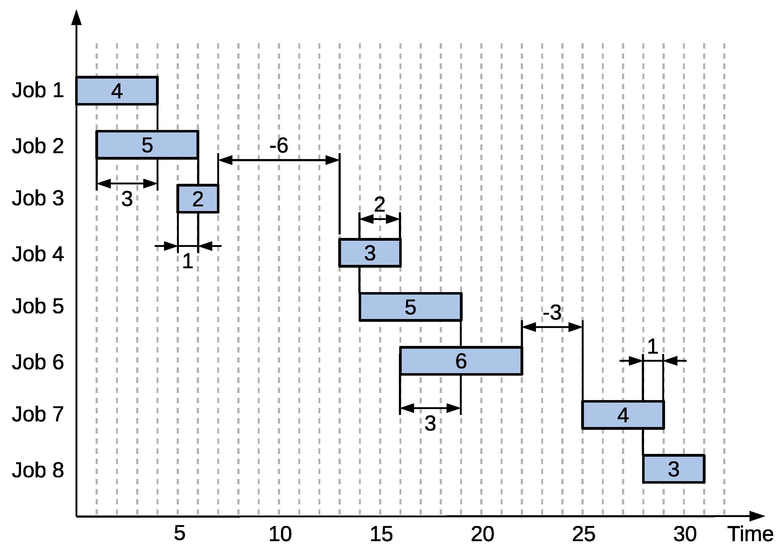
Furthermore, assume that the starting times cannot be decreased because they are constrained by completion times on the previous machine, e.g., $S_5^a=14$ cannot be decreased, because $C_5^{a-1}=14$. Furthermore, assume that the starting and completion times satisfy constraint (3). However, even under those assumptions, the considered schedule is not feasible. This can clearly be seen in Figure 2. Several jobs are overlapping each other (note that this is still a single machine: vertical differences are for easier visualization only). Indeed, for each pair of adjacent jobs, one can compute $C_i^a-S_{i+1}^a$, as indicated in the figure by the dimension lines. If the resulting distance is positive, then the jobs i and $i+1$ overlap and the job $i+1$ should be shifted to start later.

However, such a shift is not always enough. Consider the second and third jobs from Figure 2 with processing times 5 and 2, respectively. Their required shifts are 3 and 1, respectively. Shifting the third job by 1 would be enough if the second job was not shifted as well. As such, the third job needs to be shifted by 4, which is the sum of shifts values 3 and 1. The required “true” shift at job i is thus related to the sum of shifts up to that job. There is, however, an exception. Consider the fourth job. Its “local” shift is −6, while the sum of previous shifts before it is 4. A regular sum of the two would yield −2 and shift the fourth job earlier. However, the assumption was that jobs cannot decrease their starting times. Thus, the fourth job will not be shifted at all and the sum of −2 is changed to 0 instead. As a result, the sequence y of the “true” required shifts for all jobs on machine a is an inclusive scan function given by a recursive formula:

$$\begin{array}{cc}\hfill y_1& =x_1,\hfill \end{array}$$

(24)

$$\begin{array}{cc}\hfill y_i& =max\{y_{i-1}+x_i,0\}i>1,\hfill \end{array}$$

(25)

where $x_i$ is the “local” shift of job i. It should be noted that value $x_1$ (and consequently $y_1$) is zero when the entire input is considered. This is because the first job processed on the machine has no preceding job and thus will never have to be shifted in this situation. This type of scan function will be called an “inclusive job shift scan”. The exclusive variant can be defined similarly as in the case of a regular prefix sum. For the example schedule from Equations (22) and (23), the resulting “true” job shifts are thus:

$$y=(0,3,4,0,2,5,2,3).$$

(26)

After applying these shifts, the corrected feasible schedule on the machine a is obtained:

$$\begin{array}{cc}\hfill S^a& =(0,4,9,13,16,21,27,31),\hfill \end{array}$$

(27)

$$\begin{array}{cc}\hfill C^a& =(4,9,11,16,21,27,31,34).\hfill \end{array}$$

(28)

In this schedule, no jobs overlap with each other and no job was shifted earlier.

Before moving on to the next section, let us discuss the computational complexity of calculating the job shift scan. For the sequential algorithm, one directly applies Formulas (24) and (25), resulting in a running time of $O\left(n\right)$ for n jobs. As for a parallel algorithm, the first idea was to use Algorithm 2 and adjust it to the job shift scan by replacing the standard summation of $c=a+b$ with $c=max\{a+b,0\}$ as per Formulas (24) and (25). However, such an approach does not work as will be shown with another example. Let us consider the input sequence $x=(0,2,-4,3)$. According to the formulas above, the value of the last element of the job shift scan would be:

$$y_4=max\{max\{max\{0+2,0\}-4,0\}+3,0\}=3.$$

(29)

Now, it is shown that the up-sweep phase of Algorithm 2 ends with the last element of the sequence holding the total sum. For the job shift scan, this element should hold the value 3 computed above. Let us verify this by performing the phase. First, partial sums of elements $x_1$ and $x_2$ as well as $x_3$ and $x_4$ are computed. The results are $max\{0+2,0\}=2$ and $max\{-4+3,0\}=0$. Then, those partial sums are used to compute the final result $max\{2+0,0\}=2$. However, this does not match the results from (29).

The above shows that applying the base formula directly does not work for the parallel algorithm. The reason for this is that the input has been divided into two subsequences (or blocks): $(0,2)$ and $(-4,3)$. The value $-4$ is placed on the left-most side of the block, informing us how large of a shift the block is able to initially “absorb” before the actual shift takes place. However, when computing the block $(-4,3)$ on its own, the resulting value is 0 and the information of how much of a shift the block can initially absorb is lost. Even if one were to delay applying the maximum, the result of $-4+3$ is still $-1$, while in reality, the block can “absorb” the shift of 4. Since the sum of the previous block $(0,2)$ is 2, the resulting total sum remains incorrect.

The above issue can be solved as follows. We start by adding a second temporary sequence z with the same number of elements as x and y. Thus, each block of elements (jobs) i will be described by a pair of values $y_i$ and $z_i$. Value $y_i$ indicates the job shift at the end of block i (at its right-most job). This value will either be positive (shift of size $y_i$ required) or zero (no shift). On the other hand, $z_i$ will indicate the maximal shift from a preceding (“left”) block that block i is able to absorb without forcing an additional shift on the following (“right”) blocks. As such, the $z_i$ value will either be positive (absorption of a shift up to $z_i$ is possible) or zero (no absorption possible). Values $y_i$ and $z_i$ are computed simultaneously. After both sequences were determined, sequence z is discarded (it is only required through the calculation to keep track of the current absorption), while sequence y holds the required job shift scan. Thus, the previous operation in the form of:

$$max\{y_a+y_b,0\},$$

(30)

is replaced with a new operation:

$$(y_a,z_a)\oplus (y_b,z_b).$$

(31)

The remaining questions are: (1) how to define the binary operator ⊕; and (2) how to define the initial values of sequences y and z based on x. Question (2) is answered by the following Lemma.

Lemma 1.

Let $x_i$ be an element of input sequence x, i.e., $x_i$ is a block of jobs of size 1. Then, the values $y_i$ and $z_i$ describing that block are given by

$$\begin{array}{cc}\hfill y_i=& max\{x_i,0\},\hfill \end{array}$$

(32)

$$\begin{array}{cc}\hfill z_i=& max\{-x_i,0\}.\hfill \end{array}$$

(33)

Proof. 

Three cases must be considered: when $x_i$ is positive; equal to zero; and negative. When $x_i>0$, then the job overlaps with the previous one and the length of the overlapped part is $x_i$. In this case, $x_i$ is the required “local” shift, so $y_i=x_i$. Since the job itself will be shifted to the right, then no additional shift from earlier elements can be absorbed and thus the left-most absorption $z_i=0$. These results match the assumed Equations (32) and (33). When $x_i=0$, then the starting time of the job is exactly the same as the completion time of the previous job. In such a case, no shift is necessary, but any shift from the left will propagate, leaving no possibility of absorption. Thus, $y_i=z_i=0$, matching the expected values from (32) and (33). Finally, when $x_i<0$, then there is a gap from the previous job of length $x_i$. As a result, the job is not shifted, so $y_i=0$. Furthermore, due to the gap, we can absorb the shift from the left up to the size of the gap, so $z_i=x_i$. Once again, this matches the expected Equations (32) and (33). □

The above Lemma described how to initialize sequences y and z. Now, the other question is that of how to combine two adjacent blocks, i.e., how to define the operation ⊕ from (31). This was performed by the following Lemma.

Lemma 2.

Let $a=(x_i,x_{i+1},\dots ,x_{j-i},x_j)$ and $b=(x_{j+1},x_{j+2},\dots ,x_{k-1},x_k)$ where $k\ge j+1$ and $j\ge i$ be two blocks of jobs. Let these blocks be described by pairs $(y_a,z_a)$ and $(y_b,z_b)$, respectively. Then, block $c=(x_i,x_{i+1},\dots ,x_{j-i},x_j,x_{j+1},x_{j+2},\dots ,x_{k-1},x_k)$ is described by pair $(y_c,z_c)$ which is given by

$$\begin{array}{cc}\hfill y_c=& max\{y_a-z_b,0\}+y_b,\hfill \end{array}$$

(34)

$$\begin{array}{cc}\hfill z_c=& max\{z_b-y_a,0\}+z_a.\hfill \end{array}$$

(35)

Proof. 

Let us first notice that blocks a and b are continuous, i.e., block a contains all jobs from the one being processed on the considered machine as i-th to the one being processed as j-th and block b contains all jobs from the $j+1$-th to k-th. Secondly, the blocks are adjacent with block a appearing earlier, i.e., the next job being processed on the machine after processing all jobs of block a is the first job of block b.

First consider the value $z_c$. This value should be the largest shift coming from the left that the combined block c can absorb. It is known that the left-most side of c is also the left-most side of a, so c will be able to absorb at least as big of a shift as a would, hence $z_c\ge z_a$. If the shift exceeds $z_a$, then a will absorb the $z_a$ of it and the rest will propagate into block b. Block b would normally be able to absorb the shift of $z_b$, but one also needs to take into account the shift $y_a$ of block a that will be propagated into b. Three cases are possible. If $y_a=0$, then b can absorb $z_b$ and the total possible absorption of c is simply $z_a+z_b$. If $y_a>0$ but $y_a<z_b$, then b will absorb $y_a$ from a and will still be able to absorb up to $z_b-y_a$, which was not absorbed from $z_a$. The total possible absorption will then be $z_b-y_a+z_a$. Finally, if $y_a\ge z_b$, then b will use all of $z_b$ to absorb the shift from a, meaning that it will not be able to absorb any additional shift from the block preceding a, so the total absorption of c will just be $z_a$. All three cases match the expected result (35).

Now, consider the value $y_c$ in a similar manner. This value should be the total shift that will be propagated into the next block to the “right” of c. The right-most part of c is b so this shift will be at least as big as $y_b$. Now, one also needs to add the possible shift from block a. Normally, this would be $y_a$, but block b can itself absorb up to $z_b$. Once again, three subcases are possible. If $z_b=0$, then b cannot absorb anything and the entire shift $y_a$ propagates to the end of b. As a result, $y_c=y_a+y_b$. If $z_b>0$ but $z_b<y_a$, then b will absorb the shift of $z_b$ and the remainder of $y_a-z_b$ will be propagated and thus $y_c=y_a-z_b+y_b$. Finally, if $z_b\ge y_a$, then b will absorb all of $y_a$ and nothing will propagate into b, leaving $y_c=y_b$. All of these cases match the expected result (34). □

With Lemma 2, the binary relation:

$$(y_c,y_a)=(y_a,z_a)\oplus (y_b,z_b)$$

(36)

was defined through:

$$\begin{array}{cc}\hfill y_c=& max\{y_a-z_b,0\}+y_b,\hfill \end{array}$$

(37)

$$\begin{array}{cc}\hfill z_c=& max\{z_b-y_a,0\}+z_a.\hfill \end{array}$$

(38)

Before proceeding, two more properties of the binary operation ⊕, which will be required for the next step, will be proven as short corollaries below.

Corollary 1.

The binary operation $(y_a,z_a)\oplus (y_b,z_b)$ is not commutative.

Proof. 

To prove this property, it is sufficient to show a single example for which:

$$(y_a,z_a)\oplus (y_b,z_b)\ne (y_b,z_b)\oplus (y_a,z_a)$$

(39)

Let us consider:

$$(1,0)\oplus (0,1).$$

(40)

After applying the formulas from Lemma 2 one obtains $(y_c,z_c)=(0,0)$. Now, if the operands are swapped then the result is:

$$(0,1)\oplus (1,0)=(1,1)\ne \left(0.0\right).$$

(41)

□

Corollary 2.

The neutral element of the binary relation $(y_a,z_a)\oplus (y_b,z_b)$ is $(0,0)$.

Proof. 

This is trivially proven by assuming $y_a=0$ and $z_a=0$ in formulas from Lemma 2 and showing that, as a result, $y_c=y_b$ and $z_c=z_b$. Since ⊕ is not commutative, it is also done in reverse by assuming $y_b=0$ and $z_b=0$ and showing that $y_c=y_a$ and $z_c=z_a$. In both cases, the results match the expectation. □

With Lemmas 1 and 2 as well as Corollaries 1 and 2, it is now possible to propose the parallel algorithm for the job shift scan.

Theorem 1.

The job shift scan given by the recursive Formulas (24) and (25) for the input sequence $x=(x_1,x_2,\dots ,x_n)$ of n elements can be determined in time $O(logn)$ on a PRAM machine with n processors.

Proof. 

The algorithm is based on Algorithm 2, but with several changes applied. Before the start of the up-sweep phase, an additional array z with n elements is created. Since the algorithm works in-place, the array x will serve as array y. Arrays x and z are initialized as per Equations (32) and (33) from Lemma 1. It should be noted that (33) is performed first, as (32) overwrites $x_i$. Since each pair $(x_i,z_i)$ can be computed separately, this x and z initialization phase can be done in time $O\left(1\right)$ using n processors.

Then, the up-sweep phase of Algorithm 2 is conducted, which is performed the same way as for a regular prefix sum, with one exception: the + operator in line 3 is replaced with the ⊕ operator from Lemma 2. Because of this, line 3 will turn into two separate assignments. Furthermore, the value $x\left[p{2}^s\right]$ is updated first and then $z\left[p{2}^s\right]$. This is because the new value of $x\left[p{2}^s\right]$ requires the old value of $z\left[p{2}^s\right]$. This way, one avoids using temporary variables. While calculating (37) and (38) takes more time than a simple addition and assignment, it can still be achieved in time $O\left(1\right)$. Thus, the up-sweep phase can be performed in time $O(logn)$ using n processors, just as in the case of the regular prefix sum.

Before proceeding to the down-sweep phase, the last element has to be zeroed (red arrow in Figure 1. This is done by writing 0 to both $x\left[n\right]$ and $z\left[n\right]$ (as per Corollary 2). Then, the down-sweep phase starts. The copying of elements (blue arrows) is simply performed by doing both $y_i\leftarrow y_j$ and $z_i\leftarrow z_j$ for appropriate i and j values. Finally, the + operations (black arrows) once again need to be replaced with the new ⊕ operations. However, there is one difference compared with the up-sweep phase. Let us go back to Figure 1 and see how $\mathsf{\Sigma }(x_1\dots x_6)$ is computed during the down-sweep phase ($s=2$). This is done by summing $\mathsf{\Sigma }(x_5\dots x_6)$ with $\mathsf{\Sigma }(x_1\dots x_4)$. However, $\mathsf{\Sigma }(x_1\dots x_4)$, which represents earlier jobs, is on the right, while $\mathsf{\Sigma }(x_5\dots x_6)$, representing later jobs, is on the left. This property is true for the entirety of the down-sweep phase. For the regular prefix sum, it had no consequence as the + operator is commutative. However, as per Corollary 1, the ⊕ operator is not commutative. In order to fix this, one needs to swap the order of operands in line 8 of the Algorithm 2. With the presented changes, the down-sweep phase of the algorithm can be completed in time $O(logn)$ using n processors.

After the down-sweep phase is finished, array x contains the required job shift scan, while array z can be discarded. The running time of the algorithm on PRAM with n processors is $O(1+logn+logn)=O(logn)$. □

It is also easy to see that the above parallel job shift scan algorithm is work-efficient as it performs the $O\left(n\right)$ addition and maximum operations, just as the sequential version that is directly derived from Equations (24) and (25).

6. Parallel Makespan Calculation

In this section, the results of Theorem 1 as well as the parallel prefix sums will be applied to reduce the time required to compute the makespan $C_{\max }$ for the FSSP-MMI problem, as shown by the following Theorem.

Theorem 2.

Let π be a solution for the permutation flow shop problem with minimal and maximal idle time. Then, the makespan $C_{\max }\left(\pi \right)$ for π can be determined in time $O(mlogn)$ on PRAM with n processors.

Proof. 

In order to stay consistent with the nomenclature of the paper, $1,2,\dots ,n$ will be used for indexing, instead of $0,1,\dots ,n-1$. The actual implementation can use either. It is also assumed that $p_i^a$ and $C_i^a$ are matrices such that row a contains processing (or completion) times for machine a. As a reminder, $C_i^a$ takes into account the processing order $\pi$, while $p_i^a$ does not. Thus, one must remember to access ${\rho }_i^a=p_{\pi \left(i\right)}^a$ instead of $p_i^a$.

The algorithm is split into m phases, with phase a determining all values $C_i^a$ on machine a before moving onto machine $a+1$.

Phase 1 is started by performing an exclusive prefix sum of sequence $({\rho }_1^1,{\rho }_2^1,\dots ,{\rho }_n^1)$ and using sequence $C^1=(C_1^1,C_2^1,\dots ,C_n^1)$ as output. This can be done in time $O(logn)$ with Algorithm 2. After this, $C_i^1$ contains the sum of the processing times of all jobs processed on a before job i. Then, each value $C_i^1$ is modified as follows:

$$C_i^1\leftarrow C_i^1+r_1(i-1)+{\rho }_i^1.$$

(42)

The above can be calculated for each i independently, so it can be done in time $O\left(1\right)$ with n processors. The reason it is done this way is that, on the first machine, one does not have to worry about the previous machine or maximal idle time $d_1$. The jobs are “glued” together: the first job starts at time 0 and the next job starts exactly $r_1$ after the previous job is completed. The starting time of a job is thus the sum of the processing times of all jobs before it (performed by the prefix sum) plus the minimal idle time $r_1$ occurring exactly $i-1$ times (performed by (42)). However, since a completion time is needed, and not a starting time, ${\rho }_i^1$ is added as well. After this, $C^1$ holds correct completion times for machine 1, which was done in time $O(logn)$ using n processors.

Let us move onto phases 2 through m. They are more complex compared to phase 1, however, they are identical to each other, so only one of them will be described. Assume it is phase a. The phase is started as essentially identical to phase 1: the exclusive prefix sum of $({\rho }_1^a,{\rho }_2^a,\dots ,{\rho }_n^a)$ is computed, using $C^a=(C_1^a,C_2^a,\dots ,C_n^a)$ as output and corrected with:

$$C_i^a\leftarrow C_i^a+r_a(i-1)+{\rho }_i^a.$$

(43)

Essentially being the same as phase 1, the part of phase a up to this point can be performed in time $O(logn)$ using n processors.

The computed values $C_i^a$ hold completion times; however, they satisfy only the left side of constraint (5). Those starting times need to be corrected to satisfy the constraint (4). The corrections are started by performing:

$$C_i^a\leftarrow max\{C_i^a-{\rho }_i^a,C_i^{a-1}\}+{\rho }_i^a.$$

(44)

This correction is similar to the original line 7 of Algorithm 1. Furthermore, since each value $C_i^a$ can be corrected independently, this correction can be performed in time $O\left(1\right)$.

However, there is one issue with the correction (44): it is only local. If $C_i^a$ is increased by 5, while $C_{i+1}^a$ is not increased at all and the gap between the completion time of i and starting time of $i+1$ was less than 5, then the jobs will overlap. However, this is exactly the same issue which was discussed in Section 5 and Figure 2 that led to the definition of the job shift scan. Thus, this scan can be used to compute the “true” required shift and finish the correction as shown below.

First, the needed “local” jobs shifts are computed in array x of n elements as follows:

$$\begin{array}{cc}\hfill x_1& =0,\hfill \end{array}$$

(45)

$$\begin{array}{cc}\hfill x_i& =C_{i-1}^a-(C_i^a-{\rho }_i^a)-r_{a}i>1.\hfill \end{array}$$

(46)

The first job on the machine has no preceding jobs, hence $x_1=0$. For subsequent jobs, one computes the difference between the completion time of job $i-1$ (value $C_{i-1}^a$) and the starting time of job i (value $C_i^a-{\rho }_i^a$). If there is no need for a job shift, then the difference should be equal to the minimal idle time, hence the last term $r_a$. Since each element $x_i$ is computed independently, the entire array can be calculated in time $O\left(1\right)$ on n processors.

Then, the job shift scan is calculated in parallel in time $O(logn)$ with input in array $x_i$ as shown by Theorem 1. The additional arrays y and z of n elements are used, as required by this algorithm. As a result, array y now holds the “true” shifts required for each job. The only problem is that the algorithm yields the exclusive job shift scan, while an inclusive one is required. Thus, the result of the job shift scan is applied to correct the completion times $C_i^a$, while also applying Formulas (18) and (19) to obtain the inclusive scan:

$$\begin{array}{cc}\hfill C_i^a& \leftarrow C_i^a+y_{i+1},i<n\hfill \end{array}$$

(47)

$$\begin{array}{cc}\hfill C_n^a& \leftarrow C_n^a+y_L,\hfill \end{array}$$

(48)

Terms $y_{i+1}$ and $y_L$ change the exclusive job shift scan into an inclusive one, where $y_L$ is obtained through:

$$(y_L,z_L)=(y_n,z_n)\oplus (max\{x_n,0\},max\{-x_n,0\}).$$

(49)

The corrections (47)–(49) can also be done in time $O\left(1\right)$.

The phase a up to this point can be performed in time $O(logn)$. The resulting completion times $C_i^a$ satisfy all of the constraints (3)–(5) with one exception: the right side of the constraint (5), which pertains to the maximal idle time $d_a$. In other words, the phases so far give the same result as lines 1–7 from the sequential Algorithm 1. In other words, a parallel equivalent of the remaining lines 8–9 of that algorithm needs to be performed as well.

Fortunately, this last issue can be corrected in similar fashion; however, instead of preventing jobs overlapping, excessively large gaps between jobs are prevented. Specifically, one can compute the difference between the starting time of job $i+1$ and the completion time of job i. If the difference is more than $d_a$, then there is a “local” required shift for job i. Otherwise, there is no shift required, but there might be a possibility of absorption. The difference is that, previously, one block was pushed, which could result in the block to its right being pushed as well. This time, a block is being “pulled” to the next block (because there was more of a gap between them than is allowed), which might in turn force the block to its left to be “pulled” as well. Despite this “practical” difference, it is mathematically the same process. Thus, the array $x_i$ is once again prepared in time $O\left(1\right)$ as follows:

$$\begin{array}{}\mathrm{(50)}\hfill x_n& =0,\hfill \mathrm{(51)}\hfill x_{n-i+1}& =C_{i+1}^a-{\rho }_{i+1}^a-C_i^a-d_{a}i>1.\hfill \end{array}$$

As one can see, this time the array is prepared a little differently. This is because previously the first job always had a 0 shift and then shifts propagated from left to right. This time, the last job n has no required shift and “pulls” propagate from right to left. Thus, the direction has to be changed. The simplest way to do this is to prepare the input x from the other end, which allows using the same parallel job shift scan as previously, which will be completed in time $O(logn)$. After obtaining the job shift scan (using arrays y and z), the correction is applied, remembering to reverse the direction back and change the scan from exclusive to inclusive:

$$\begin{array}{}\mathrm{(52)}\hfill C_i^a& \leftarrow C_i^a+y_{n-i+1},i>1\hfill \mathrm{(53)}\hfill C_1^a& \leftarrow C_1^a+y_L,\hfill \end{array}$$

where $y_L$ is obtained as before. This correction is done in time $O\left(1\right)$. After this, all completion times in sequence $C^a$ are correct and phase a ends. All operations in phase a had a running time of either $O\left(1\right)$ or $O(logn)$ thus the entire phase can be completed in time $O(logn)$ using n processors.

After phase m was completed, the value of the makespan is equal to $C_n^m$. Since any phase (including phase 1) can be done in time $O(logn)$ and there are m phases, in conclusion, the algorithm runs in time $O(mlogn)$ on PRAM with n processors. □

It should be noted that, while the results of Theorem 1 were employed to calculate the goal function for FSSP-MMI, the job shift scan has wider applications. It could be used for a multitude of scheduling problems with precedence constraints (need for pushing or pulling jobs according to some rules with propagation in place). Similar results could be obtained for scheduling problems with limited wait constraints or setup times, for example. In particular, this result can be employed for classic and widely-used FSSPs with any method that requires recalculating the makespan from scratch. Such a situation arises, for example, with genetic operators in many Genetic Algorithm-based approaches to scheduling.

7. Solving Method

This section describes the implementation of the solving method for the FSSP-MMI. The chosen method is the simulated annealing (SA) metaheuristic, which has been successfully applied to a variety of FSSPs and similar scheduling problems both over the years [62,63] and recently [64,65,66].

7.1. Base SA Implementation

SA is an iterative local search metaheuristic that employs the concept of a neighborhood. At each iteration, a neighbor ${\pi }^{\prime }$ of the current solution $\pi$ is generated and evaluated. If ${\pi }^{\prime }$ is better than $\pi$ (for our problem, this means that $C_{\max }\left({\pi }^{\prime }\right)<C_{\max }\left(\pi \right)$) then ${\pi }^{\prime }$ is accepted and replaces $\pi$. Otherwise, ${\pi }^{\prime }$ can still be accepted with a probability based on the goal function of the neighbor and a parameter called temperature. An initial temperature is chosen and every set number of iterations E (called epoch) the temperature generally decreases according to the chosen cooling schedule. At the beginning, at a higher temperature, worse solutions are more readily accepted, allowing for diversification. When the temperature becomes lower, the algorithm starts to focus on exploring the current portion of the solution space (intensification). In general, in order to implement SA for our FSSP problem, we need to decide the following:

• Solution representation;
• Definition of neighborhood;
• Initial temperature and cooling schedule;
• Initial solution;
• Acceptance function;
• Stopping condition.

The typical structure of the SA method is shown in Algorithm 3.

Algorithm 3 Outline of the simulated annealing metaheuristic

The following SA implementation was used. The processing order $\pi$ was employed as a solution representation. As for the neighborhood, the swap neighborhood was chosen, i.e., a neighbor ${\pi }^{\prime }$ was created from $\pi$ by swapping elements $\pi \left(i\right)$ and $\pi \left(j\right)$ with each other, where $i\in \mathcal{J}$ and $j\in \mathcal{J}\setminus \left\{i\right\}$ are chosen randomly. The initial temperature was set as follows. k random solutions were generated. Let ${\pi }_b$ and ${\pi }_w$ be the best and worst among those k solutions. Then, the initial temperature t is set to:

$$t\leftarrow \frac{C_{\max }\left({\pi }_w\right)-C_{\max }\left({\pi }_b\right)}{n}.$$

(54)

As for the cooling schedule, the standard geometric one was employed. The following temperature is given as $\alpha t$, where $\alpha \in (0;1)$ and t is the previous temperature. The initial solution $\pi$ is chosen as a random permutation of sequence $\{1,2,\dots ,n\}$. The acceptance probability of a neighbor solution ${\pi }^{\prime }$ is given as

$$e^{\frac{C_{\max }\left(\pi \right)-C_{\max }\left({\pi }^{\prime }\right)}{t}}.$$

(55)

In order for the algorithm to be applicable for large problem sizes and as a local-search subroutine for other solving methods, a time limit was chosen as the stopping condition. More specifically, the algorithm stops and returns the best found solution ${\pi }^{\ast }$ after:

$$\frac{nm}{51.2}$$

(56)

milliseconds. This way, for 1024 jobs and 50 machines, the running time is one second. After preliminary research, the parameters were set to $k=20$, $E=10$ and $\alpha =0.9999$.

7.2. SA Variants and CUDA Implementation

The last missing part of the solving method is the implementation of the subroutine that computes the goal function. In fact, three variants of the SA metaheuristic were developed—two sequential and one parallel:

• SAC: in this variant, the entire algorithm is executed on CPU using a single thread;
• SAG: in this variant, the goal function is computed on GPU using a single thread. The rest of the algorithm is run on CPU using a single thread;
• SAP: in this variant, the goal function is computed on GPU in parallel using n threads. The rest of the algorithm is run on CPU using a single thread.

The implementation of the goal function computation for SAC is straightforward, directly employing Algorithm 1. Since no accelerator for quickly computing the goal function of the neighbor ${\pi }^{\prime }$ is known, the makespan has to be recomputed from scratch in time $O\left(nm\right)$. The rest of the algorithm follows the outline of Algorithm 3. No GPU resources are used and thus no CPU–GPU transfers occur. All memory is allocated on the host and most of it is dynamic allocation.

The implementation of the SAG variant is similar. The same sequential Algorithm 1 is used, except the computation is performed by running a CUDA kernel with one thread. Data such as matrices $p_i^a$ and $C_i^a$ are copied into the GPU memory only once at the start of the algorithm. The data are not copied from the GPU back to the CPU, except for obtaining the value of $C_{\max }$ (by copying $C_n^m$) and for assigning an improved $\pi$ to ${\pi }^{\ast }$. The generation of ${\pi }^{\prime }$ is performed by swapping two elements in $\pi$ on GPU (in time $O\left(1\right)$) with the CPU code providing which elements to swap. If ${\pi }^{\prime }$ is not accepted, then the elements are simply swapped back to restore $\pi$. This variant uses a global GPU memory plus some local variables. As a result, the goal function calculation is done in time $O\left(nm\right)$ as for the SAC variant.

The implementation of the SAP variant is the most complex. The makespan $C_{\max }$ is generally computed by implementing Theorem 2. Specific parts of it (prefix sums, job shift scan, input preparation, corrections) are performed by running CUDA kernels with a number of blocks. A single block runs 256 threads and each thread handles two elements, yielding 512 elements handled per block.

Most of the operations required to compute the makespan, such as (42)–(44), can be performed in time $O\left(1\right)$ through simple kernel functions that run a necessary number of blocks. This is because the computation for each element are independent. However, the computation of prefix sums and job shift scans is more complex, as results from one block impact the sum/scan further on in subsequent blocks.

To solve this issue, the parallel prefix sum was implemented following the implementation shown by Harris et al. [67]. First, the prefix sum computation for a single block is implemented, following Algorithm 2.The problem instance is first allocated on CPU and then allocated and copied to the GPU global memory. It is important to note that this happens only once at the beginning of the entire SAP solving method. The CUDA kernels that run in time $O\left(1\right)$ use this global memory (plus some local variables). However, kernels used for computing the prefix sum and job shift scan use the GPU shared memory, which is faster. Data are copied from the appropriate parts of the global memory into the shared memory (which is only visible to the given thread block). The kernel then works on that shared memory (plus local variables) and the results are copied into appropriate global memory locations (possibly different from the input location) before the kernel terminates. Furthermore, to increase performance and prevent memory access conflicts from bottle-necking the kernel, memory coalescing is used, avoiding memory bank conflicts. This is performed in a manner presented in [67].

The above algorithm is then extended to a number of jobs n larger than double the size of a block. This is performed as follows. Multiple blocks are run at once (as many as necessary, given n) and the prefix sum is computed independently. This will not affect the total complexity, which will remain at $O(logn)$), as long as the GPU has enough parallel resources to run all such blocks in parallel.

The problem with independent calculation is that each block i starts summing from 0 instead of the sum of all previous elements in previous blocks. To fix this, one needs to know the (inclusive) sum of all elements prior to that block, which is obtained as follows. First, Algorithm 2 is slightly modified, such that at the end of the up-sweep phase and before the zeroing of the last element, the value of that last element (which is the total sum of the given input sequence) is stored in another array $\mathit{sums}$ at index i, which is the number of the block. After executing this modified algorithm for k blocks, $\mathit{sums}\left[i\right]$ will contain the total sum of elements in block i. A prefix sum is performed again, this time on $\mathit{sums}$ alone (which is a single block) and the result is stored in yet another array $\mathit{incr}$. This way, $\mathit{incr}\left[i\right]$ holds the total sum of all elements in the blocks before i. A simple CUDA kernel can now be used to add the value of $\mathit{incr}\left[i\right]$ to every element of block i for all blocks in time $O\left(1\right)$. It should also be noted that additional arrays $\mathit{sums}$ and $\mathit{incr}$ are in global memory, but when the prefix sum kernel is launched, those arrays are only used as the starting input and final output. All other kernel operations were performed using fast shared block memory and local variables. For additional information on efficient prefix sum computation on CUDA, please consult [67] (accessible via PDF).

One disadvantage of this approach is that $\mathit{sums}$ is the size of one block, which limits this method to 512 blocks. This approach thus cannot currently handle problems with more than $512\times 512$ = 262,144 jobs. An extension that would enable larger problem sizes is possible, but would likely affect the performance.

The job shift scan is similarly implemented to the prefix sum, except the operator ⊕ is employed instead of +. This also means that the additional arrays z, $z_{\mathit{sums}}$ and $z_{\mathit{incr}}$ are required. The same global-shared memory and bank conflicts considerations as with the prefix sum apply. Moreover, CUDA is used to update the best-known solution ${\pi }^{\ast }$. Namely, for SAC and SAG variants, one must copy it with a single thread in time $O\left(n\right)$. For the SAP variant, it can be copied in time $O\left(1\right)$ using n processors via a simple CUDA kernel. Due to this, for SAG, all solutions are kept on the GPU throughout the algorithm and the final best solution is copied back to CPU memory only once at the end of the algorithm.

8. Computer Experiment

In this section, the results of computer experiments to measure the parallel speedup of the proposed solving methods as well as some of its subroutines are described. The problem instances generation, the experiment setting and the measure of quality for comparing different variants of the SA metaheuristic will also be described.

Considering the testing environment and software used, all programs were written in C/C++ in Visual Studio 2019 version 16.10.2 and compiled using the Release configuration. All programs were run on a server with the AMD Ryzen Threadripper 3990X CPU (2.9 MHz, 64-cores), 64 GB of RAM and an RTX 2080 Ti GPU (1.35 GHz, 11 GB memory, 4352 CUDA cores) in the Microsoft Windows 10 Pro operating system.

In the first experiment, the speedups obtained for several subroutines are shown. At first, for comparison, the results of the implementation of the parallel prefix sum calculation are presented. For each input length n, an array of n integers of random values were created. The prefix sum calculation was then executed on CPU, the GPU with the single thread and GPU with n threads, obtaining the running times $T_C$, $T_G$ and $T_P$, respectively. Since the running times were small, the computation was repeated a number of times depending on n (e.g., 400,000 times for $n=16$ and 25 times for n = 262,144) and the total running time was measured. After this, the obtained total was divided by the number of repetitions. The measured running times (in milliseconds) and speedups of the parallel version against both sequential versions are shown in

Table 2. Running times and speedups for the CPU (C); GPU sequential (G); and GPU parallel (P) prefix sum calculation.

n	${\mathit{T}}_{\mathbf{P}}$ (ms)	${\mathit{T}}_{\mathbf{G}}$ (ms)	${\mathit{T}}_{\mathbf{C}}$ (ms)	${\mathit{T}}_{\mathbf{G}}/{\mathit{T}}_{\mathbf{P}}$	${\mathit{T}}_{\mathbf{C}}/{\mathit{T}}_{\mathbf{P}}$
16	3.188	2.797	0.006	0.8773	0.0018
32	3.072	3.132	0.012	1.0194	0.0038
64	3.187	4.109	0.024	1.2893	0.0074
128	3.326	6.179	0.053	1.8578	0.0159
256	3.598	10.108	0.103	2.8090	0.0285
512	3.930	18.632	0.193	4.7412	0.0491
1024	10.426	35.743	0.418	3.4284	0.0401
2048	10.287	69.497	0.791	6.7560	0.0769
4096	10.390	136.973	1.590	13.1836	0.1531
8192	10.644	274.419	3.172	25.7813	0.2980
16,384	10.438	546.239	6.403	52.3338	0.6135
32,768	11.404	1090.091	12.765	95.5884	1.1193
65,536	11.646	2177.404	25.574	186.9658	2.1959
131,072	15.742	4370.652	51.094	277.6427	3.2457
262,144	25.332	8901.572	115.372	351.3963	4.5544

.

It can be observed that the speedup compared to the sequential GPU was already visible at $n=32$ elements with the maximal speedup of over 350 at n = 262,144. Compared to the CPU, the speedups are much lower both due to the lower GPU core speeds as well as the overhead of the executing CUDA kernels. Nonetheless, speedups against CPU are observed for $n>$ 32,768 with a maximal speedup of 4.55. This is similar to the speedup reported by Harris et al. for the same n [67].

The next experiment concerns the running times and speedups of the job shift scan from Theorem 1 and the goal function calculation from Theorem 2. Similar experiments as with the prefix sums were performed but with a different number of repetitions. For the makespan calculation $m=10$ was assumed. Such a number of machines allowed to lessen the effect of the constant overhead, while also keeping the computation time reasonable. Reporting the running times of the sequential GPU and CPU versions was omitted, as they can be derived from the speedup. The results are shown in

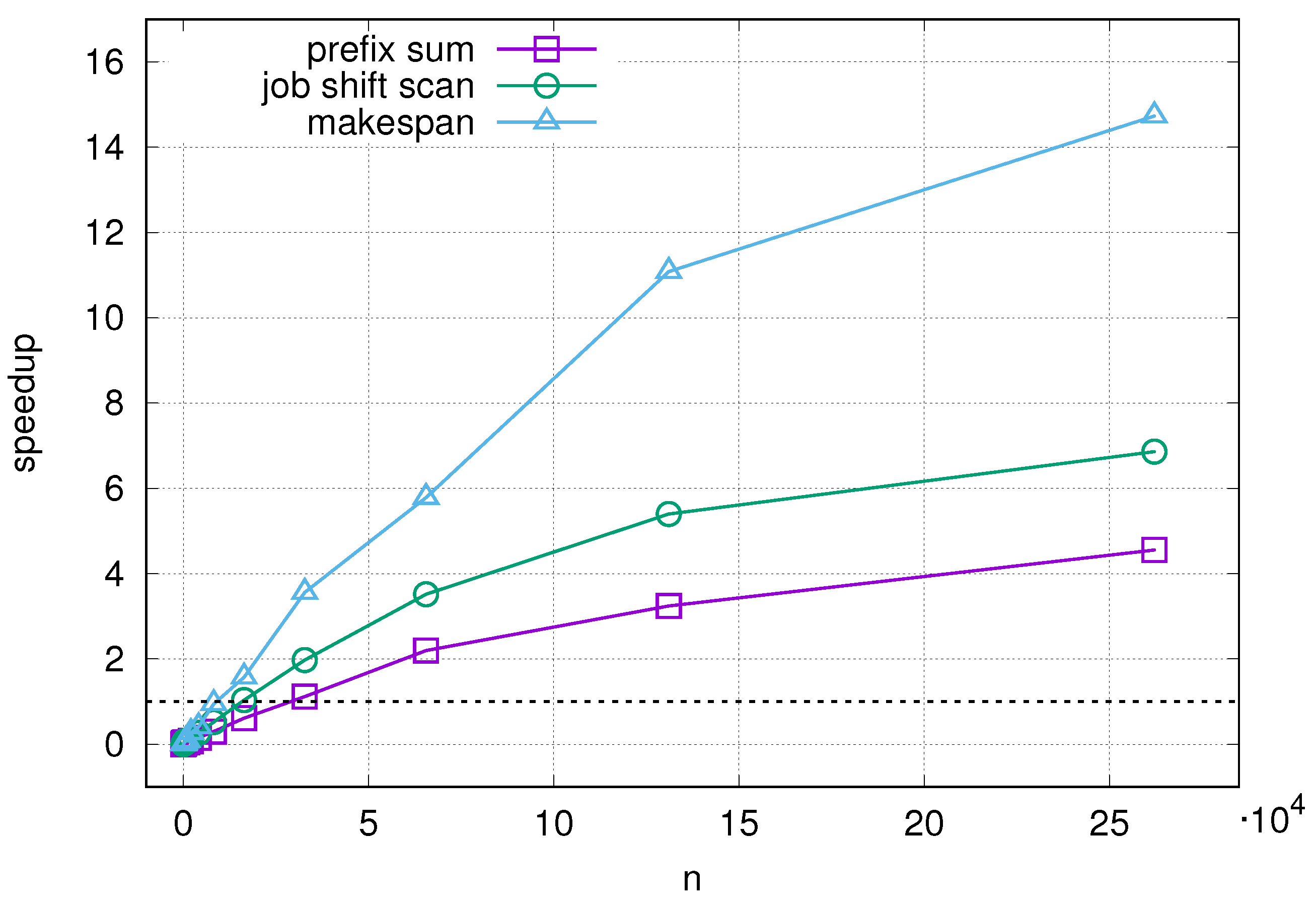
Table 3. Running times and speedups for CPU (C); GPU sequential (G); and GPU parallel (P) job shift scan and makespan calculations.

n	Job Shift Scan			Makespan ($\mathit{m}=10$)
	${\mathit{T}}_{\mathit{P}}$ (ms)	${\mathit{T}}_{\mathbf{G}}/{\mathit{T}}_{\mathbf{P}}$	${\mathit{T}}_{\mathbf{C}}/{\mathit{T}}_{\mathbf{P}}$	${\mathit{T}}_{\mathit{P}}$ (ms)	${\mathit{T}}_{\mathbf{G}}/{\mathit{T}}_{\mathbf{P}}$	${\mathit{T}}_{\mathbf{C}}/{\mathit{T}}_{\mathbf{P}}$
16	3.225	0.883	0.003	205.426	0.130	0.002
32	3.131	1.027	0.006	212.864	0.244	0.005
64	3.398	1.237	0.013	220.033	0.465	0.010
128	3.660	1.732	0.026	220.901	0.918	0.016
256	3.934	2.783	0.049	225.090	1.801	0.034
512	4.619	4.299	0.082	243.333	3.326	0.071
1024	11.690	3.284	0.065	438.464	3.750	0.087
2048	11.846	6.344	0.129	445.268	7.431	0.267
4096	11.602	12.811	0.263	446.554	16.062	0.406
8192	11.689	25.316	0.522	438.007	37.452	0.946
16,384	11.768	50.107	1.036	442.908	106.487	1.574
32,768	12.490	94.155	1.975	462.183	242.515	3.563
65,536	13.667	172.511	3.517	528.990	448.940	5.786
131,072	18.387	257.059	5.401	632.542	768.073	11.083
262,144	28.738	331.854	6.861	978.860	1029.311	14.732

.

The computation times and speedups against the sequential GPU for the job shift scan are comparable to those for the prefix sum from Table 2. Speedups against the CPU are observed for $n>$ 16,384 with the top speedup of over 6.8. The results for the makespan calculation, however, are more surprising. Even though this procedure relies on the prefix sum and jobs shift scan, the observed speedups are vastly different. The speedup against GPU is lower at first (observable from approximately $n=140$), but becomes much higher, with over 1000 for n = 262,144. Similarly, against CPU, the speedup is obtained from approximately $n=9000$ and the highest speedup observed is over 14.7. However, one possible explanation for this result is that most of the CUDA kernels launched during the makespan computation work in time $O\left(1\right)$ instead of $O(logn)$—further increasing the perceived speedup. The speedups obtained for the prefix sum, job shift scan and makespan calculations against the GPU and CPU are shown in Figure 3 and Figure 4.

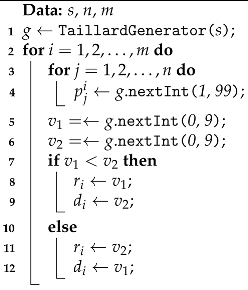
Then, research was conducted to compare the SAC, SAG and SAP variants of the SA metaheuristic. As for problem instances, 12 instances groups were prepared with $n\times m$ sizes from $32\times 5$ to 65,536 × 300. The reason for choosing such an instance size was both to consider large-scale problems (for cloud scheduling and Big Data applications), as well as to research the limitations of the speedup achievable with this method. For each instance group, 10 instances were prepared (as in the original Taillard scheme), yielding 120 instances in total. Each instance was generated using the pseudo-random number generator used by Taillard [68], which is often used, with slight modification, by researchers, in order to stay consistent with Taillard’s original instances. The generation procedure is shown in Algorithm 4. The same 120 seed values as in Taillard’s were used.

Algorithm 4 Instance generation procedure

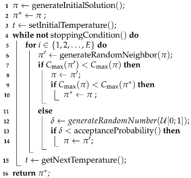
All three SA variants have a time limit as their stopping conditions, thus, the comparison will be based on the quality of solutions (makespan values) the variants are able to provide in that time limit. In order to compare instances of vastly different sizes, the percentage relative deviation (PRD) was chosen as the quality measure. Assuming that $\pi$ is a solution provided by the given algorithm for the given instance, then PRD is defined as

$$100\%\frac{C_{\max }\left({\pi }_{\mathrm{ref}}\right)-C_{\max }\left(\pi \right)}{C_{\max }\left({\pi }_{\mathrm{ref}}\right)},$$

(57)

where ${\pi }_{\mathrm{ref}}$ is a reference solution. Ideally, this would be the optimal solution, but it can be also a best-known or arbitrary solution. In this research, the parallel variant (SAP) will be compared with the sequential variants (SAG and SAC), therefore:

$${\mathrm{PRD}}_G=100\%\frac{C_{\max }\left({\pi }_{\mathrm{G}}\right)-C_{\max }\left({\pi }_{\mathrm{P}}\right)}{C_{\max }\left({\pi }_{\mathrm{G}}\right)},$$

(58)

$${\mathrm{PRD}}_C=100\%\frac{C_{\max }\left({\pi }_{\mathrm{C}}\right)-C_{\max }\left({\pi }_{\mathrm{P}}\right)}{C_{\max }\left({\pi }_{\mathrm{C}}\right)},$$

(59)

where ${\pi }_{\mathrm{P}}$, ${\pi }_{\mathrm{G}}$, ${\pi }_{\mathrm{C}}$ are the solutions found by the SAP, SAG and SAC variants, respectively. Furthermore, ${\mathrm{it}}_P$, ${\mathrm{it}}_G$ and ${\mathrm{it}}_C$ denote the number of iterations performed by the SAP, SAG and SAC variants, respectively.

Since SA is a probabilistic method, every instance was executed 10 times and the results are shown in

Table 4. Averaged PRD and numbers of iteration elapsed for 120 Taillard-based instances using SAP, SAG and SAC variants.

$\mathit{n}\times \mathit{m}$	${\mathbf{PRD}}_{\mathbf{G}}$ (%)	${\mathbf{PRD}}_{\mathbf{C}}$ (%)	${\mathbf{it}}_{\mathit{P}}/{\mathbf{it}}_{\mathit{G}}$	${\mathbf{it}}_{\mathit{P}}/{\mathbf{it}}_{\mathit{C}}$	${\mathbf{it}}_{\mathit{P}}$
32 × 5	$-0.628$	$-9.804$	0.565	0.002	11.0
64 × 10	$-2.235$	$-11.911$	0.487	0.006	32.8
128 × 10	$-0.181$	$-7.191$	0.953	0.015	82.7
256 × 30	2.806	$-9.653$	1.793	0.037	196.7
512 × 30	4.129	$-5.071$	3.435	0.071	377.9
1024 × 50	4.248	$-5.320$	4.020	0.088	442.2
2048 × 70	4.845	$-3.061$	8.201	0.184	902.1
4096 × 100	3.744	$-1.289$	18.317	0.372	1813.4
8192 × 150	3.055	$-0.253$	47.147	0.746	3630.3
16,384 × 200	2.021	0.294	130.396	1.638	7171.8
32,768 × 250	1.411	0.425	312.465	3.248	13,748.5
65,536 × 300	0.853	0.363	665.518	5.980	24,892.9

. Each value is an average out of 100 runs (10 instances, 10 repeats for instance). As expected, the SAP variant is able to perform more iterations in the given time limit starting at approximately $n=140$. At $n=$ 65,536, the SAP is able to complete 665 times more iterations than SAG. Similarly, from approximately $n=$ 11,000, the SAP variant performs more iterations than SAC, with almost as many as six times more at $n=$ 65,536. By executing more iterations, the SAP variant provided makespans shorter by up to 5% on average compared to the SAG variant, with the highest average improvement (4.8%) observed for $n=2048$. The improvement when compared with the SAC variant is much smaller (under 0.5%), but still noticeable.

9. Conclusions and Future Work

In this paper, a permutation flow shop scheduling problem with minimal and maximal machine idle times and a makespan criterion was considered. A custom prefix sum-like operation called a job shift scan for correcting the completion times of jobs for scheduling problems was proposed. A binary operator that realizes the job shift scan was proposed and its properties, including commutability, were discussed. A work-efficient parallel algorithm for computing the job shift scan for the PRAM model was proposed and its logarithmic running time with regard to the number of jobs was proven. Prefix sums and job shift scans were then used to propose a parallel algorithm for calculating the makespan in the time $O(mlogn)$. Based on the above, an implementation of the job shift scan and makespan calculation algorithm for the CUDA platform was proposed.

The results of the computer experiment indicated large GPU-to-GPU speedups of up to 330 and 1030 times for the job shift scan and the makespan calculation, respectively, as well as significant GPU-to-CPU speedups of up to 7 and 14 times. A simulated annealing metaheuristic algorithm for the considered problem was then proposed. Experiments using Taillard-based instances proved that, for sufficiently large problems, the parallel variant of the algorithm performed more iterations in the given time limit and allowed to obtain shorter makespans. With the proposed algorithm, it is possible to solve large-size problem instances in acceptable time or reduce the running time of the algorithm, allowing it to be used as a local-search procedure in other methods.

For future work, two research directions were considered. The first was to extend the approach to different scheduling problems. The second was to implement the proposed algorithm purely on manycore CPU instead of GPU, for the possibility of further increasing the speedup and avoiding CPU–GPU copying and kernel launch overhead.

References

1. Burcin Ozsoydan, F.; Sağir, M. Iterated greedy algorithms enhanced by hyper-heuristic based learning for hybrid flexible flowshop scheduling problem with sequence dependent setup times: A case study at a manufacturing plant. Comput. Oper. Res. 2021, 125, 105044. [Google Scholar] [CrossRef]
2. Du, J.; Dong, P.; Sugumaran, V. Dynamic Production Scheduling for Prefabricated Components Considering the Demand Fluctuation. Intell. Autom. Soft Comput. 2020, 26, 715–723. [Google Scholar] [CrossRef]
3. Rogalska, M.; Hejducki, Z. The application of time coupling methods in the engineering of construction projects. Tech. Trans. 2017, 114, 67–74. [Google Scholar] [CrossRef]
4. Tong, Z.; Chen, H.; Deng, X.; Li, K.; Li, K. A scheduling scheme in the cloud computing environment using deep Q-learning. Inf. Sci. 2020, 512, 1170–1191. [Google Scholar] [CrossRef]
5. Chhabra, A.; Singh, G.; Kahlon, K.S. QoS-Aware Energy-Efficient Task Scheduling on HPC Cloud Infrastructures Using Swarm-Intelligence Meta-Heuristics. Comput. Mater. Contin. 2020, 64, 813–834. [Google Scholar] [CrossRef]
6. Yao, E.; Liu, T.; Lu, T.; Yang, Y. Optimization of electric vehicle scheduling with multiple vehicle types in public transport. Sustain. Cities Soc. 2020, 52, 101862. [Google Scholar] [CrossRef]
7. Bassen, J.; Balaji, B.; Schaarschmidt, M.; Thille, C.; Painter, J.; Zimmaro, D.; Games, A.; Fast, E.; Mitchell, J.C. Reinforcement Learning for the Adaptive Scheduling of Educational Activities. In Proceedings of the 2020 CHI Conference on Human Factors in Computing Systems; Association for Computing Machinery: New York, NY, USA, 2020; pp. 1–12. [Google Scholar] [CrossRef]
8. Amindoust, A.; Asadpour, M.; Shirmohammadi, S. A Hybrid Genetic Algorithm for Nurse Scheduling Problem considering the Fatigue Factor. J. Healthc. Eng. 2021, 2021, 5563651. [Google Scholar] [CrossRef] [PubMed]
9. Harki, N.; Ahmed, A.; Haji, L. CPU scheduling techniques: A review on novel approaches strategy and performance assessment. J. Appl. Sci. Technol. Trends 2020, 1, 48–55. [Google Scholar] [CrossRef]
10. Liu, Z.; Qiu, X.; Zhang, S.; Deng, S.; Liu, G. Service Scheduling Based on Edge Computing for Power Distribution IoT. Comput. Mater. Contin. 2020, 62, 1351–1364. [Google Scholar] [CrossRef]
11. Chang, X.; Xu, X.; Yang, D. Pipeline Scheduling Based on Constructive Interference in Strip Wireless Sensor Networks. Comput. Mater. Contin. 2020, 64, 193–206. [Google Scholar] [CrossRef]
12. Yuan, S.; Li, T.; Wang, B. A discrete differential evolution algorithm for flow shop group scheduling problem with sequence-dependent setup and transportation times. J. Intell. Manuf. 2021, 32, 427–439. [Google Scholar] [CrossRef]
13. Ruiz, R.; Stützle, T. An Iterated Greedy heuristic for the sequence dependent setup times flowshop problem with makespan and weighted tardiness objectives. Eur. J. Oper. Res. 2008, 187, 1143–1159. [Google Scholar] [CrossRef]
14. Thürer, M.; Ma, L.; Stevenson, M. Workload Control order release in general and pure flow shops with limited buffer size induced blocking: An assessment by simulation. Int. J. Prod. Res. 2021, 59, 2558–2569. [Google Scholar] [CrossRef]
15. Harbaoui, H.; Khalfallah, S.; Bellenguez-Morineau, O. A case study of a hybrid flow shop with no-wait and limited idle time to minimize material waste. In Proceedings of the 2017 IEEE 15th International Symposium on Intelligent Systems and Informatics (SISY), Subotica, Serbia, 14–16 September 2017; pp. 207–212. [Google Scholar] [CrossRef]
16. Ni, F.; Hao, J.; Lu, J.; Tong, X.; Yuan, M.; Duan, J.; Ma, Y.; He, K. A Multi-Graph Attributed Reinforcement Learning Based Optimization Algorithm for Large-Scale Hybrid Flow Shop Scheduling Problem. In Proceedings of the 27th ACM SIGKDD Conference on Knowledge Discovery & Data Mining, KDD ’21; Association for Computing Machinery: New York, NY, USA, 2021; pp. 3441–3451. [Google Scholar] [CrossRef]
17. Zhao, F.; He, X.; Zhang, Y.; Lei, W.; Ma, W.; Zhang, C.; Song, H. A jigsaw puzzle inspired algorithm for solving large-scale no-wait flow shop scheduling problems. Appl. Intell. 2020, 50, 87–100. [Google Scholar] [CrossRef]
18. Ma, T.; Pang, S.; Zhang, W.; Hao, S. Virtual Machine Based on Genetic Algorithm Used in Time and Power Oriented Cloud Computing Task Scheduling. Intell. Autom. Soft Comput. 2019, 25, 605–613. [Google Scholar] [CrossRef]
19. Rudy, J.; Smutnicki, C. Online scheduling for a Testing-as-a-Service system. Bull. Pol. Acad. Sci. Tech. Sci. 2020, 68. [Google Scholar] [CrossRef]
20. Gmys, J. Solving large permutation flow-shop scheduling problems on GPU-accelerated supercomputers. arXiv 2020, arXiv:2012.09511. [Google Scholar]
21. Bozejko, W.; Wodecki, M. Solving the flow shop problem by parallel tabu search. In Proceedings of the International Conference on Parallel Computing in Electrical Engineering, Warsaw, Poland, 22–25 September 2002; pp. 189–194. [Google Scholar] [CrossRef]
22. Bożejko, W.; Uchroński, M.; Wodecki, M. Fast Parallel Cost Function Calculation for the Flow Shop Scheduling Problem. In Artificial Intelligence and Soft Computing; Rutkowski, L., Korytkowski, M., Scherer, R., Tadeusiewicz, R., Zadeh, L.A., Zurada, J.M., Eds.; Springer: Berlin/Heidelberg, Germany, 2012; pp. 378–386. [Google Scholar]
23. Idzikowski, R.; Rudy, J.; Gnatowski, A. Solving Non-Permutation Flow Shop Scheduling Problem with Time Couplings. Appl. Sci. 2021, 11, 4425. [Google Scholar] [CrossRef]
24. Zaied, A.N.H.; Ismail, M.M.; Mohamed, S.S. Permutation Flow Shop Scheduling Problem with Makespan Criterion: Literature Review. J. Theor. Appl. Inf. Technol. 2021, 99, 830–848. [Google Scholar]
25. Bożejko, W.; Rudy, J.; Idzikowski, R. Parallel Computing for the Non-permutation Flow Shop Scheduling Problem with Time Couplings Using Floyd-Warshall Algorithm. In Performance Evaluation Models for Distributed Service Networks; Bocewicz, G., Pempera, J., Toporkov, V., Eds.; Springer: Cham, Switzerland, 2021; pp. 1–19. [Google Scholar]
26. Kim, Y.D.; Joo, B.J.; Shin, J.H. Heuristics for a two-stage hybrid flowshop scheduling problem with ready times and a product-mix ratio constraint. J. Heuristics 2009, 15, 19–42. [Google Scholar] [CrossRef]
27. Choi, S.W. Optimal Scheduling Algorithms to Minimize Total Flowtime on a Two–Machine Permutation Flowshop with Limited Waiting Times and Ready Times of Jobs. Int. J. Appl. Eng. Res. 2017, 12, 5101–5109. [Google Scholar]
28. Arroyo, J.E.C.; Leung, J.Y.T. An effective iterated greedy algorithm for scheduling unrelated parallel batch machines with non-identical capacities and unequal ready times. Comput. Ind. Eng. 2017, 105, 84–100. [Google Scholar] [CrossRef]
29. Jiang, X.; Guan, N.; Long, X.; Tang, Y.; He, Q. Real-time scheduling of parallel tasks with tight deadlines. J. Syst. Archit. 2020, 108, 101742. [Google Scholar] [CrossRef]
30. Yağmur, E.; Kesen, S.E. A memetic algorithm for joint production and distribution scheduling with due dates. Comput. Ind. Eng. 2020, 142, 106342. [Google Scholar] [CrossRef]
31. Kianpour, P.; Gupta, D.; Krishnan, K.K.; Gopalakrishnan, B. Automated job shop scheduling with dynamic processing times and due dates using project management and industry 4.0. J. Ind. Prod. Eng. 2021, 1–14. [Google Scholar] [CrossRef]
32. Jafarzadeh, H.; Moradinasab, N.; Gerami, A. Solving no-wait two-stage flexible flow shop scheduling problem with unrelated parallel machines and rework time by the adjusted discrete Multi Objective Invasive Weed Optimization and fuzzy dominance approach. J. Ind. Eng. Manag. (JIEM) 2017, 10, 887–918. [Google Scholar] [CrossRef] [Green Version]
33. Koulamas, C.; Kyparisis, G.J. The no-wait flow shop with rejection. Int. J. Prod. Res. 2021, 59, 1852–1859. [Google Scholar] [CrossRef]
34. Engin, O.; Güçlü, A. A new hybrid ant colony optimization algorithm for solving the no-wait flow shop scheduling problems. Appl. Soft Comput. 2018, 72, 166–176. [Google Scholar] [CrossRef]
35. Wu, X.; Che, A. Energy-efficient no-wait permutation flow shop scheduling by adaptive multi-objective variable neighborhood search. Omega 2020, 94, 102117. [Google Scholar] [CrossRef]
36. Santosa, B.; Siswanto, N. Discrete particle swarm optimization to solve multi-objective limited-wait hybrid flow shop scheduling problem. IOP Conf. Ser. Mater. Sci. Eng. 2018, 337, 012006. [Google Scholar] [CrossRef] [Green Version]
37. Dhouib, E.; Teghem, J.; Loukil, T. Non-permutation flowshop scheduling problem with minimal and maximal time lags: Theoretical study and heuristic. Ann. Oper. Res. 2018, 267, 101–134. [Google Scholar] [CrossRef]
38. Fondrevelle, J.; Oulamara, A.; Portmann, M.C. Permutation flowshop scheduling problems with maximal and minimal time lags. Comput. Oper. Res. 2006, 33, 1540–1556. [Google Scholar] [CrossRef]
39. Yuan, S.; Li, T.; Wang, B. A co-evolutionary genetic algorithm for the two-machine flow shop group scheduling problem with job-related blocking and transportation times. Expert Syst. Appl. 2020, 152, 113360. [Google Scholar] [CrossRef]
40. Ribas, I.; Companys, R.; Tort-Martorell, X. An iterated greedy algorithm for the parallel blocking flow shop scheduling problem and sequence-dependent setup times. Expert Syst. Appl. 2021, 184, 115535. [Google Scholar] [CrossRef]
41. Harbaoui, H.; Khalfallah, S. Tabu-search optimization approach for no-wait hybrid flow-shop scheduling with dedicated machines. Procedia Comput. Sci. 2020, 176, 706–712. [Google Scholar] [CrossRef]
42. Zhao, F.; Zhang, L.; Zhang, Y.; Ma, W.; Zhang, C.; Song, H. A hybrid discrete water wave optimization algorithm for the no-idle flowshop scheduling problem with total tardiness criterion. Expert Syst. Appl. 2020, 146, 113166. [Google Scholar] [CrossRef]
43. Rossi, F.L.; Nagano, M.S. Heuristics for the mixed no-idle flowshop with sequence-dependent setup times and total flowtime criterion. Expert Syst. Appl. 2019, 125, 40–54. [Google Scholar] [CrossRef]
44. Della Croce, F.; Grosso, A.; Salassa, F. Minimizing total completion time in the two-machine no-idle no-wait flow shop problem. J. Heuristics 2019, 1–15. [Google Scholar] [CrossRef]
45. Czapiński, M.; Barnes, S. Tabu Search with two approaches to parallel flowshop evaluation on CUDA platform. J. Parallel Distrib. Comput. 2011, 71, 802–811. [Google Scholar] [CrossRef] [Green Version]
46. Bożejko, W. Solving the flow shop problem by parallel programming. J. Parallel Distrib. Comput. 2009, 69, 470–481. [Google Scholar] [CrossRef]
47. Smutnicki, C.; Pempera, J.; Rudy, J.; Żelazny, D. A new approach for multi-criteria scheduling. Comput. Ind. Eng. 2015, 90, 212–220. [Google Scholar] [CrossRef]
48. Bożejko, W.; Gnatowski, A.; Pempera, J.; Wodecki, M. Parallel tabu search for the cyclic job shop scheduling problem. Comput. Ind. Eng. 2017, 113, 512–524. [Google Scholar] [CrossRef]
49. Rudy, J.; Pempera, J.; Smutnicki, C. Improving the TSAB algorithm through parallel computing. Arch. Control. Sci. 2020, 411–435. [Google Scholar] [CrossRef]
50. Rudy, J.; Żelazny, D. GACO: A parallel evolutionary approach to multi-objective scheduling. In International Conference on Evolutionary Multi-Criterion Optimization; Springer: Berlin/Heidelberg, Germany, 2015; pp. 307–320. [Google Scholar] [CrossRef]
51. Borisovsky, P.; Kovalenko, Y. A Memetic Algorithm with Parallel Local Search for Flowshop Scheduling Problems. In Bioinspired Optimization Methods and Their Applications; Filipič, B., Minisci, E., Vasile, M., Eds.; Springer International Publishing: Cham, Switzerland, 2020; pp. 201–213. [Google Scholar]
52. Wei, K.C.; Sun, X.; Chu, H.; Wu, C.C. Reconstructing permutation table to improve the Tabu Search for the PFSP on GPU. J. Supercomput. 2017, 73, 4711–4738. [Google Scholar] [CrossRef]
53. Luo, J.; Baz, D.E.; Hu, J. Acceleration of a CUDA-Based Hybrid Genetic Algorithm and its Application to a Flexible Flow Shop Scheduling Problem. In Proceedings of the 2018 19th IEEE/ACIS International Conference on Software Engineering, Artificial Intelligence, Networking and Parallel/Distributed Computing (SNPD), Busan, Korea, 27–29 June 2018; pp. 117–122. [Google Scholar] [CrossRef] [Green Version]
54. Luo, J.; Fujimura, S.; El Baz, D.; Plazolles, B. GPU based parallel genetic algorithm for solving an energy efficient dynamic flexible flow shop scheduling problem. J. Parallel Distrib. Comput. 2019, 133, 244–257. [Google Scholar] [CrossRef] [Green Version]
55. Luo, J.; El Baz, D. A dual heterogeneous island genetic algorithm for solving large size flexible flow shop scheduling problems on hybrid multicore CPU and GPU platforms. Math. Probl. Eng. 2019, 2019, 1713636. [Google Scholar] [CrossRef]
56. Coelho, P.; Silva, C. Parallel Metaheuristics for Shop Scheduling: Enabling Industry 4.0. Procedia Comput. Sci. 2021, 180, 778–786. [Google Scholar] [CrossRef]
57. Blelloch, G.E. Prefix Sums and Their Applications; Technical Report; Citeseer: Princeton, NJ, USA, 1990. [Google Scholar]
58. Yang, Y.; Wu, Y.; Pan, J. Parallel Dynamics Computation Using Prefix Sum Operations. IEEE Robot. Autom. Lett. 2017, 2, 1296–1303. [Google Scholar] [CrossRef] [Green Version]
59. Nunes, L.S.N.; Bordim, J.L.; Ito, Y.; Nakano, K. A Prefix-Sum-Based Rabin-Karp Implementation for Multiple Pattern Matching on GPGPU. In Proceedings of the 2018 Sixth International Symposium on Computing and Networking (CANDAR), Takayama, Japan, 27–30 November 2018; pp. 139–145. [Google Scholar] [CrossRef]
60. Kohlhoff, K.J.; Pande, V.S.; Altman, R.B. K-Means for Parallel Architectures Using All-Prefix-Sum Sorting and Updating Steps. IEEE Trans. Parallel Distrib. Syst. 2013, 24, 1602–1612. [Google Scholar] [CrossRef]
61. Hillis, W.D.; Steele, G.L. Data Parallel Algorithms. Commun. ACM 1986, 29, 1170–1183. [Google Scholar] [CrossRef]
62. van Laarhoven, P.J.M.; Aarts, E.H.L.; Lenstra, J.K. Job Shop Scheduling by Simulated Annealing. Oper. Res. 1992, 40, 113–125. [Google Scholar] [CrossRef] [Green Version]
63. Osman, I.; Potts, C. Simulated annealing for permutation flow-shop scheduling. Omega 1989, 17, 551–557. [Google Scholar] [CrossRef]
64. Ying, K.C.; Lin, S.W. Solving no-wait job-shop scheduling problems using a multi-start simulated annealing with bi-directional shift timetabling algorithm. Comput. Ind. Eng. 2020, 146, 106615. [Google Scholar] [CrossRef]
65. Wei, H.; Li, S.; Jiang, H.; Hu, J.; Hu, J. Hybrid Genetic Simulated Annealing Algorithm for Improved Flow Shop Scheduling with Makespan Criterion. Appl. Sci. 2018, 8, 2621. [Google Scholar] [CrossRef] [Green Version]
66. Lin, S.W.; Cheng, C.Y.; Pourhejazy, P.; Ying, K.C. Multi-temperature simulated annealing for optimizing mixed-blocking permutation flowshop scheduling problems. Expert Syst. Appl. 2021, 165, 113837. [Google Scholar] [CrossRef]
67. Harris, M.; Sengupta, S.; Owens, J.D. Parallel prefix sum (scan) with CUDA. GPU Gems 2007, 3, 851–876. [Google Scholar]
68. Taillard, E. Benchmarks for basic scheduling problems. Eur. J. Oper. Res. 1993, 64, 278–285. [Google Scholar] [CrossRef]
Figure 1. Work-efficient exclusive parallel prefix sum computation algorithm for k = 8 .
Applsci 11 08204 g001
Figure 2. Exemplary schedule on a machine with some overlapping jobs. The required “local” job starting times shifts are shown.
Applsci 11 08204 g002
Figure 3. Measured GPU vs. GPU speedups as a function of the number of jobs for the prefix sum, job shift scan and makespan.
Applsci 11 08204 g003
Figure 4. Measured GPU vs. CPU speedups as a function of the number of jobs for the prefix sum, job shift scan and makespan. Black dashed line indicates a speedup of 1.0.
Applsci 11 08204 g004