Probabilistic Analysis as a Method for Ground Freezing Depth Estimation

Abstract

Accurate frost depth prediction is an important aspect in different engineering designs such as for pavements, buildings, bridge foundations, and utility lines. This paper presents a probabilistic method of assessment of the depth of soil freezing. Annual (winter) maxima of the position of the zero centigrade temperature measured in the soil were approximated by Gumbel probability distribution. Its parameters were estimated using maximum likelihood method. The results received on the basis of data from 36 meteorological stations in Poland and 50 years of observations, as characteristic values with 50-year return period, reflect the influence of the climatic conditions on the freezing depth. On the other hand, the soil structure and its conditions also play an important role in freezing. Nowadays they may be taken into account using correction coefficients. It is concluded that this method is more precise than a method using the air freezing index because through the use of direct measurements it takes into account additional factors affecting the actual depth of freezing. The obtained results are not the same as those given in the older Polish Standard which was based on the simplified and limited data. The results confirm the impact of climate change on ground freezing depth.

1. Introduction

Freezing of the soil in wintertime is one of the climatic actions which must be considered when designing structures founded on soils. The actual frost depth is affected by the material type, soil thermal properties, soil water content, and climatic conditions such as temperature, wind speed, precipitation, and solar radiation. Frost depth can be estimated using numerical or analytical modeling technique (Gontaszewska [1], Konrad & Shen [2], Rajaei & Baladi [3], Venäläinen et al. [4], ). In the past few years different numerical techniques have been used for modeling transient heat flow in pavement layers. These methods require a large number of input data [4,5]. In most cases the input data are either not available or just too expensive to collect. In the case of missing data, higher or similar accuracy can be obtained from simpler analytical and semi-empirical models to estimate frost depth prediction—for e.g., Stefan model, modified Berggren model or Chisholm and Phang empirical model [3,5]. In those methods, the depth of frost penetration has usually been defined using the so-called air freezing index. However, it is obvious that the frost penetration into the soil is a complex random process in which many factors affect the final results, which are often divergent from the observations [6]. Those are not only air temperature but also the depth and the thermal properties of snow cover, which is changing during winter, heat contained in the soil [7,8] and the soil properties, its structure and water content. All the climatic conditions have a random character and should be analyzed using probabilistic methods. Nowadays, the simplest approach is the probabilistic analysis of the annual (winter) maximum depth of the zero centigrade temperature. However, it should be emphasized that it is not the same as the depth of the soil freezing. The purpose of the paper is to present the probabilistic analysis of the maximum annual depth of the zero centigrade temperature of the soils, the implemented method and some examples of the obtained results.

Since 1955, the maps of the soil freezing depths have been given in Polish Standards. The values were calculated in centimeters according to the formula given in Soviet recommendations [9]:

$$h_z=23\cdot \sqrt{{\displaystyle \sum m+2}}$$

(1)

where: m—an absolute value of the winter monthly mean negative air temperature; only negative values are summarized.

The numerical factor 23 means the type of soil. The value 23 is for loams and clays. Numbers for other types of soil were not given in the Polish Standards. According to Zavarina [10], this formula was derived on the basis of the experiments made at six Soviet meteorological stations. A similar formula but with more detail was elaborated at the US Army Cold Regions Research and Engineering Laboratory [6].

The results of the calculations according to the Formula (1) were implemented into the Polish Standard in 1955 (PN-55/B-03020) and its next editions with small modification in 1974. For the western half of Poland, the depth of freezing was 0.8 m, for the eastern part it was 1.0 m and for small area around Suwałki region it was 1.4 m.

The approach, based on the air freezing index, is still recommended [1]. However, now it is possible to define the depth of the zero centigrade temperature on the basis of direct measurements of the soil temperature.

2. Material and Methodology

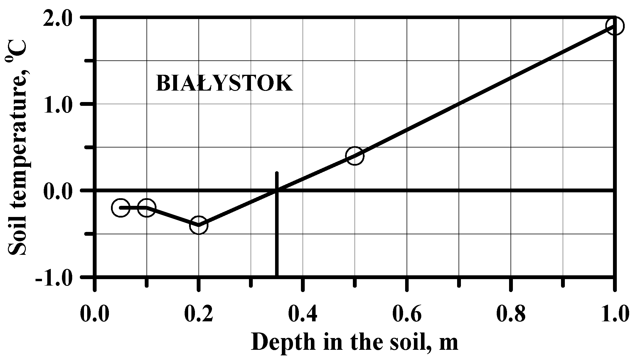
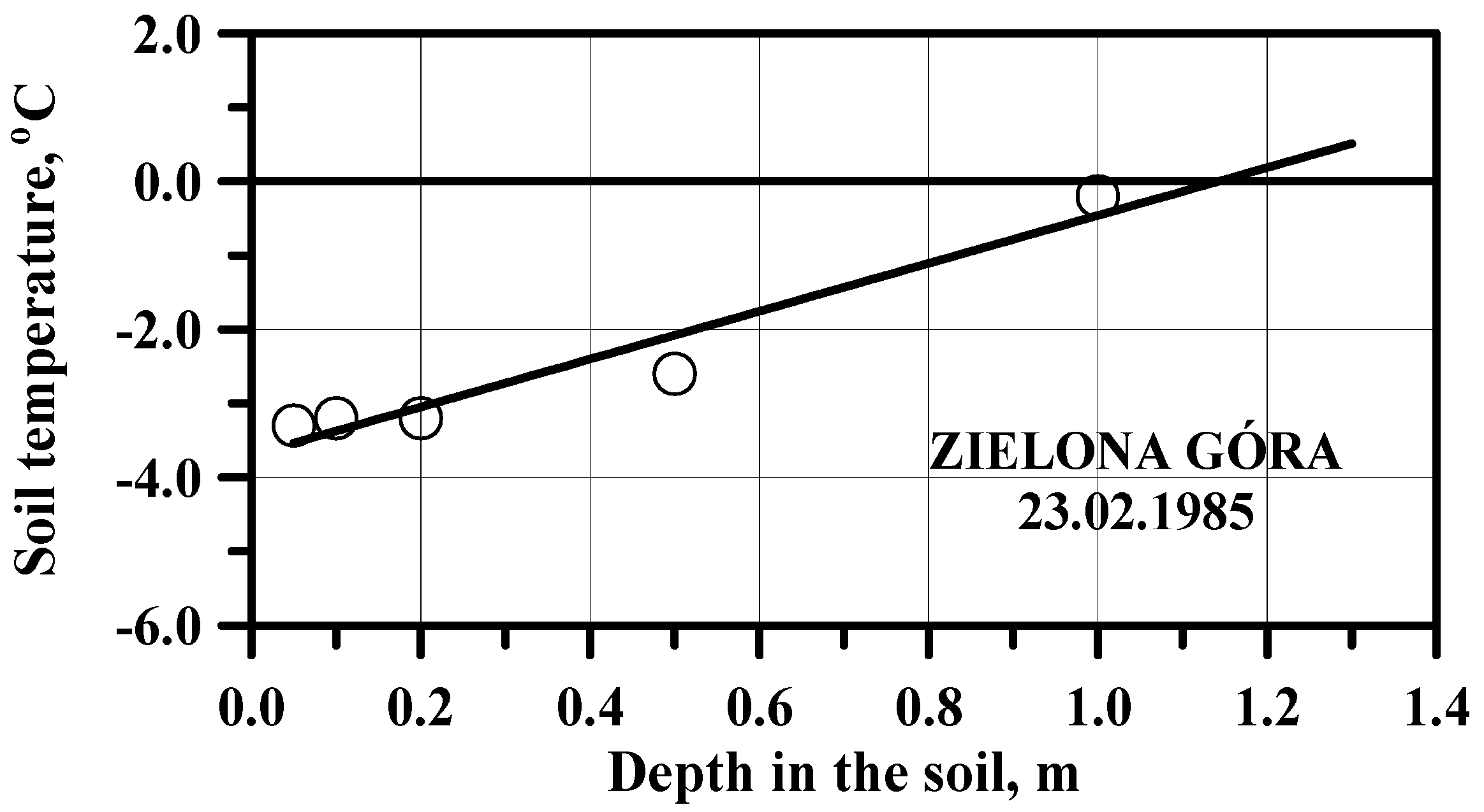
2.1. Measurements of Soil Temperature

The Earth’s surface is heated by the absorption of solar radiation. The variety of the substrate results in different heating mechanism. Snow and ice covering the ground reflects most of the radiation [11]. Water, due to its partial transparency, absorbs radiation throughout the layer to which it reaches, and the ground absorbs radiation in a thin surface layer [12]. Changes in ground temperature depend on its vegetation coverage, chemical composition, and to a large extent on water and air content. The source of heat in the ground can also be heat exchange with the atmosphere; thawing and freezing processes of water contained in the ground; precipitation heat and biological, chemical, and physical processes in the soil [13]. Soil, which is not covered with vegetation, is most strongly heated during the day in clear weather; at night in the same conditions, it intensely radiates heat. The size of the heat flux absorbed or given away by the soil depends on the temperature difference and the thermal capacity of the soil [14,15]. The thermal capacity of the soil is influenced by its mineral composition, water and air content. There is a very large impact of the snow cover on the depth of the zero isotherm position. The maximum positions of zero isotherms in the ground without snow cover are even more than twice as deep as in snow-covered soils [16,17].

Soil freezing (frost) depth can be determined using a number of direct approaches, for example, by direct measurement by thermometers installed in the ground. Another approach is to use the concept of ‘degree days’—freezing degree days (FDDs) and thawing degree days (TDDs)—as a surrogate for frost depth. The advantage of the ‘degree day’ approach is that meteorological data is easier to obtain and less intrusive than the other described approaches. A limitation of the degree-day approach is the representativeness of temperature data taken off-site [18].

In Poland, the soil temperature is measured every day at the meteorological stations of the Institute for Meteorology and Water Management—State Research Institute (IMGW-PIB). The measurements were taken in the last 40 years using mercury-in-glass thermometers, at 6:00 and 18:00 UTC at the depths of 5 cm, 10 cm, 20 cm, and 50 cm and at the depth of 1.0 m but only at 12:00 UTC [19]. Measurements at this last depth have been made only since 1982. Currently, the measurements are automated, performed every minute with an accuracy of 0.1 °C. Measurements of the minimum temperature above the surface of the exposed soil and the ground temperature are made on the testing site. This measuring field is a part of the ground with area of 2 × 4 m; the longer sides of the plot are directed in the direction E-W. Experimental plot are free of the grass. The measurement technique for the soil temperature and the method of calculation of the zero centigrade depth were described in the instruction for meteorological measurements [20,21].

Freezing the ground is a physical process consisting of the freezing of water present in the ground and its molecules into a hard permafrost. The water contained in the soil is a solution of different salts of varying concentrations, the higher their concentration, the lower the ground freezing temperature. This temperature may drop to −2 °C and below. Freezing of the ground depends on the air temperature, the duration of the negative temperatures, the thickness and type of snow cover, the terrain profile, and the structure and humidity of the ground. The low air temperature that persists for a long time lowers the temperature of deeper and deeper layers of the ground, while strong but short-term temperature drops have less impact on the freezing depth of the ground. An important role is played by the snow cover: a thicker, less dense and even layer of snow inhibits the process of freezing the ground. Different types of soils are characterized by different ease of freezing. The process of ground freezing consists of solar radiation, the advection of warm air masses, and heat penetrating from deeper layers of soil. The timing of freezing of the first layers of soil, the length of permafrost persistence and the maximum freezing depth are of great importance in construction, agriculture, and water management. At weather stations measuring ground temperature at depths of 5, 10, 20, 50, and 100 cm, isotherm “0” in the ground is calculated. Isotherm (E_T) “0” is the plane connecting the points at 0 °C in the ground [19]. Depending on the course of the weather, there may be one or more “0” isotherms in the ground. On the basis of measured everyday values of soil temperature personnel of weather stations calculate the position of the zero centigrade temperature. Following formula is used:

$$Z=A+\frac{a\cdot \mathsf{\Delta }{T}_A}{\mathsf{\Delta }T}$$

(2)

where: A—the depth of the lowest place of thermometer which measured negative temperature; a—the distance between depths of thermometers measuring negative and positive temperature; ΔT_A—temperature at the level A; ΔT—the difference between temperature values at the levels with zero centigrade temperature between them.

An example is presented in Figure 1 below: A = 0.2 m, a = 0.5 − 0.2 = 0.3 m, ΔT_A = −0.4 °C, ΔT = −0.8 °C. Zero-degree temperature is at the depth of 0.35 m.

The problem may occur when the negative soil temperature exceeds 1.0 m depth. In such a case it is recorded as below 1.0 m. The true value can be defined using extrapolation of values measured at smaller depths. An example is presented in Figure 2. However, it must be pointed out that such cases were not frequent.

When determining the position of a zero isotherm by extrapolation, it should be taken into account that as the temperature rises in the upper layers of the ground at an unchanged value at the depth of the largest measurement, the slope of the straight regression decreases. The use of such a set may lead to an error in the determination of the extrapolated value.

2.2. Methods of Probabilistic Analysis

The aim of the analysis is to find such values of the position of zero centigrade temperature which would be exceeded with the accepted probability in appropriate reference period. Nowadays, the commonly accepted annual probability of exceedance of climatic actions is 0.02 which means 50-year return period. Such an assumption may also be used for the probabilistic calculation of freezing depths. The probability that a value Z_k will be exceeded once in t years is:

$$P\left(Z>Z_k\right)=\frac{1}{t}$$

(3)

and the probability of not exceeding it is:

$$P\left(Z\le Z_k\right)=1-\frac{1}{t}=F\left(Z_k\right)$$

(4)

In order to find Z_k one has to use the annual (winter) maxima of the position of the zero centigrade temperature and the appropriate probability distribution. The Gumbel distribution [22] has been preferred here. The Gumbel extreme—value distribution was used to analyze the data on locations of the zero isotherm. The purpose of this study was to fit an extreme-value distribution to a given set of winter maxima of soil freezing depth denoted by Z_i. The cumulative distribution function (CDF) is given as:

$$F(Z)=\exp \left\{-\exp \left[-\alpha \left(Z-U\right)\right]\right\}$$

(5)

where: α and U are parameters of the distribution estimated using the maximum likelihood method.

This distribution and procedure have been widely used to forecast wind velocity and snow load, e.g., [23]. It was also used to forecast soil freezing [24]. After being doubly logarithmized, it takes the form of a linear function with respect to α, U. The value Z_k of the depth of zero centigrade temperature and 50-year return period is calculated using the following equation:

$$Z=U-\frac{1}{\alpha }\ln \left[-\ln F\left(Z\right)\right]$$

(6)

The unknown Gumbel distribution parameters (α, U) were estimated using the least squares method, the maximum likelihood method, the method of moments, and the method described by Julius Lieblein in his work [25].

2.3. Estimation of Gumbel Distribution Parameters

In order to determine the parameters, the measurement results are depicted on the Gumbel probability grid depending on the position each observation occupies in the statistics order. The measurement results are treated as the values of the function which arguments have the form, where the ordinal number is in the ascending order of the n-element measurement data set [26].

2.3.1. Least Square Estimation

This method is relatively easy to use as double logarithm of Gumbel distribution results in the equation of a straight line. The parameters of the regression function are approximations of the Gumbel distribution parameters. Good approximation is obtained when noticeable linear relationship is present. The estimation method of Gumbel distribution parameters based on the least square method gives the best results as the coefficient of correlation R ≥ 0.95. However, it is very sensitive to the cases when some points are located far outside the straight line. Such cases are often occurring, for example, in snow load on the ground. Such points are increasing the steepness of the regression line, which leads to the overestimation of the predicted values. In extreme cases, the linear regression do not fit the approximated empirical distribution at all, which then disqualifies this method.

The straight line was fitted to the points placed on the probability grid so that it runs as close as possible to all points, i.e., the sum of the squares of vertical distance of points from this straight line is as small as possible. The inverse of the slope coefficient of this line and its Z-intercept are the parameters of the Gumbel distribution—being the results of the least squares estimation (LSM).

2.3.2. Maximum Likelihood Method

Maximum likelihood estimation is recommended due to its many advantages. In this method, the assessment of the estimated parameters is based on values maximizing the credibility of the sample. Due to the lack of analytical solution for assessment of the distribution parameters, numerical methods are used. Estimators obtained with this method are consistent, asymptotically most efficient and they have normal asymptotical distribution. In practice, this method is rarely used due to calculation complexity, as the values of parameter distribution are assessed iteratively. The implementation of the maximum likelihood method (Max LM) consisted of seeking the maximum of the likelihood function given by the formula:

$$l={\displaystyle \prod _{i=1}^n\alpha \cdot \exp \left\{-\alpha \left(Z_i-U\right)-\exp \left[-\alpha \left(Z_i-U\right)\right]\right\}}$$

(7)

The values α, U for which the Function (7) reaches its global maximum are the parameters of the Gumbel distribution estimated by the maximum likelihood method.

2.3.3. Method of Moments

The moment method is simpler. In order to determine the parameters (α, U) using the method of moments, certain sample moments referring to measured values Z_i were compared to the corresponding moments of the Gumbel distribution [27,28]. The arithmetic mean $Z_m$ and variance ${\sigma }^2$ as properties of the Gumbel distribution are expressed by the following formulas:

$$Z_m=U+\frac{1}{\alpha }·\gamma ,\hspace{1em}{\sigma }^2=\frac{{\pi }^2}{6\cdot {\alpha }^2}$$

(8)

where: γ = 0.5772 is the Euler constant.

Comparing the Formulas (8) to corresponding quantities related to the n-element sample of winter maxima of freezing depth, we obtain the values α, U of the Gumbel distribution parameters estimated by the method of moments (MM).

2.3.4. Lieblein Method—BLUE

Julius Lieblein [25] proposed a method of estimating Gumbel distribution parameters based on order statistics, requiring the sample elements Z_i to be placed in ascending order. The estimators of the investigated distribution parameters take the form of a linear function with respect to positional statistics:

$${\widehat{b}}_{(n)}=\frac{1}{{\widehat{\alpha }}_{(n)}}={\displaystyle \sum _{i=1}^n{b}_i{Z}_i},\hspace{1em}\widehat{U}={\displaystyle \sum _{i=1}^n{a}_i{Z}_i}$$

(9)

where: Best Linear Unbiased Estimators (BLUE) are with minimal variance. The coefficients $b_i, a_i$ were collated in the paper [25] for sample size of $n=1,2,\dots ,16$. The aforementioned work also describes a method of estimating parameters $b, U$ for arbitrarily large sample with a size of n having given coefficients for an m-element sample if m < n. For an n-element sample, the coefficients $b_i^{\prime }, a_i^{\prime }$ can be calculated using the following formulas:

$$\begin{array}{c}{b}_i^{\prime }={\displaystyle \sum }_{j=1}^m{b}_j\cdot \left(j/i\right)p\left(n,m,i,j\right),\hfill \\ i=1,2,\dots ,n\hfill \\ a_i^{\prime }={\displaystyle \sum }_{j=1}^m{a}_j\cdot \left(j/i\right)p\left(n,m,i,j\right),\hfill \end{array}$$

(10)

where:

$$p\left(n,m,i,j\right)=\left(\begin{array}{c}i\\ j\end{array}\right)\left(\begin{array}{c}n-i\\ m-j\end{array}\right)/\left(\begin{array}{c}n\\ m\end{array}\right)$$

(11)

is the hypergeometric probability function. The formulas below allow the calculation of “good” estimators ${\widehat{b}}_{(n)}^{\prime }, {\widehat{U}}_{(n)}^{\prime }$ for an n-element sample:

$${\widehat{b}}_{(n)}^{\prime }=\frac{1}{{\widehat{\alpha }}_{(n)}^{\prime }}={\displaystyle \sum _{i=1}^n{b}_i^{\prime }\cdot Z_i},\hspace{1em}{\widehat{U}}_{(n)}^{\prime }={\displaystyle \sum _{i=1}^n{a}_i^{\prime }\cdot Z_i}$$

(12)

The samples analyzed in this work contain significantly more than 16 measurement results; therefore, a set of BLUE coefficients b_j, a_j for m = 16 was used in the calculations.

The evaluation of the results obtained with four methods proved to be more difficult than the estimation of the Gumbel distribution parameters. As we have four Gumbel distributions, we face the question which of them best approximates the empirical distribution and can be used to determine the characteristic value Z_k of the location of the zero isotherm in the ground [26]. The test statistics of chi-squared, Kolmogorov–Smirnov and Cramer von Mises were adopted as a measure of adjustment of the theoretical to the empirical distribution. Low values of these statistics indicate that the given theoretical distribution truly reflects the empirical distribution.

Amid the known compliance tests, the chi squared test is mentioned first. It requires the decomposition of the Z axis into $r+1$ intervals $I_1,\hspace{1em}{I}_2,\hspace{1em}\cdots ,\hspace{1em}{I}_{r+1}$ by the numbers $-\infty =g_0<g_1<\cdots <g_r<g_{r+1}=\infty .$ The difference in the value of the cumulative distribution function $F$ at the ends of the interval is equal to the probability $p$ that the random variable Z will take a value belonging to that interval:

$$p_j=F\left(g_j\right)-F\left(g_{j-1}\right), j=1,2,\dots ,r+1$$

(13)

The chi squared test statistic for a measurement sequence consisting of n maximum freezing depths is given by the formula:

$${\chi }^2={\displaystyle \sum _{j=1}^{r+1}\frac{{\left(n_j-n{p}_j\right)}^2}{n{p}_j}}$$

(14)

where: n_j—the number of measured values of Z within I_j, while np_j—is the expected number of measurement results which, according to the considered distribution, should be in I_j [29]. An examination of distribution compliance by means of statistics (14) leaves the choice of the number of intervals I_j into which the axis Z is divided and the points g_j constituting the limits of these intervals. In this work because of the ambiguity mentioned chi-squared test was implemented in two variants. The first one assumes the division of the Z variable axis into one-element intervals, the limits of which are arithmetic means of two values adjacent in the order statistics. The only exception here are points g₀, g_r+1 equal to minus and plus infinity, respectively. In the second variant, the division into five intervals with equal probability p_j was used. Point g₁ was set as the arithmetic mean of the fifth and sixth elements in a series of ascending order data: g₁ = (Z₅ + Z₆)/2. The value of the cumulative distribution function at point g₁ is equal to the probability of the first interval: F(g₁) = p. The same probability of all intervals is ensured by the next boundary points g_j being defined as:

$$g_j=U-\frac{1}{\alpha }\ln \left[-\ln \left(p+F\left(g_{j-1}\right)\right)\right],\dots j=1,2,\cdots ,r$$

(15)

except the last: $g_{r+1}=\infty .$

Other tests refer to hypothetical cumulative distribution function and verify its compliance with empirical cumulative distribution function. Kolmogorov–Smirnov statistics D_n1 verifies the quality of the adjustment on the basis of the largest absolute value of the hypothetical F(Z) and empirical F_n(Z) cumulative distribution function difference:

$$D_{n1}=\underset{z}{\sup }\left|F_n\left(Z\right)-F\left(Z\right)\right|$$

(16)

In Formula (16), unlike in [30], the $\sqrt{n}$ factor is omitted, because only equally numerous sets of values $F_n\left(Z\right)$ and $F\left(Z\right)$ are compared with each other and without any reference to samples of a different size $n.$ Another variation of Kolmogorov–Smirnov statistics found in the literature was also used, namely:

$$D_n^{+}=\underset{1\le i\le n}{\max }\left|\frac{i}{n}-F\left(Z_{i:n}\right)\right|,\hspace{1em}{D}_n^{-}=\underset{1\le i\le n}{\max }\left|F\left(Z_{i:n}\right)-\frac{i-1}{n}\right|$$

(17)

from where:

$$D_{n2}=\max \left\{D_n^{+},\hspace{1em}{D}_n^{-}\right\}$$

(18)

The above Formulas (16)–(18) define the maximum discrepancy between the postulated Gumbel distribution and the measured depths of the zero isotherm location. So, the idea arose to do a similar check for medium differences of hypothetical and geometrical cumulative distribution function. The subsequent tests are equivalent to statistics (16)–(18) and check not the maximum, but the average distance of the hypothetical and empirical cumulative distribution function. According to this reasoning, statistics (16) representing the average spacing of the cumulative distribution function is given by the formula:

$$D_{n1s}={\displaystyle \sum _{i=1}^n\frac{\left|F_n\left(Z_i\right)-F\left(Z_i\right)\right|}{n}}$$

(19)

Whereas the equivalent of statistics (18) in relation to the average value is expressed by the formulas:

$$D_n^{+}=\frac{1}{n}{\displaystyle \sum _{i=1}^n\left|\frac{i}{n}-F\left(Z_{i:n}\right)\right|},\hspace{1em}{D}_n^{-}=\frac{1}{n}{\displaystyle \sum _{i=1}^n\left|F\left(Z_{i:n}\right)-\frac{i-1}{n}\right|}$$

(20)

and next:

$$D_{n2s}=\frac{1}{2}\left(D_n^{+}+D_n^{-}\right)$$

(21)

Another test used in this work, comparing the cumulative distribution function with order statistics of measurement results, is Cramer von Mises’s statistics [31] in the form:

$$W_{CM}=\frac{1}{12n}+{{\displaystyle \sum _{i=1}^n\left(F\left(Z_i\right)-\frac{2i-1}{2n}\right)}}^2$$

(22)

The best estimation method was considered to be the one indicated by most of the mentioned tests. For example, if the chi squared statistic is the smallest for the Gumbel distribution parameters $\alpha ,U$ determined by the maximum likelihood method, it means that the chi squared test indicates the maximum likelihood method as the best of four applied methods.

3. Results

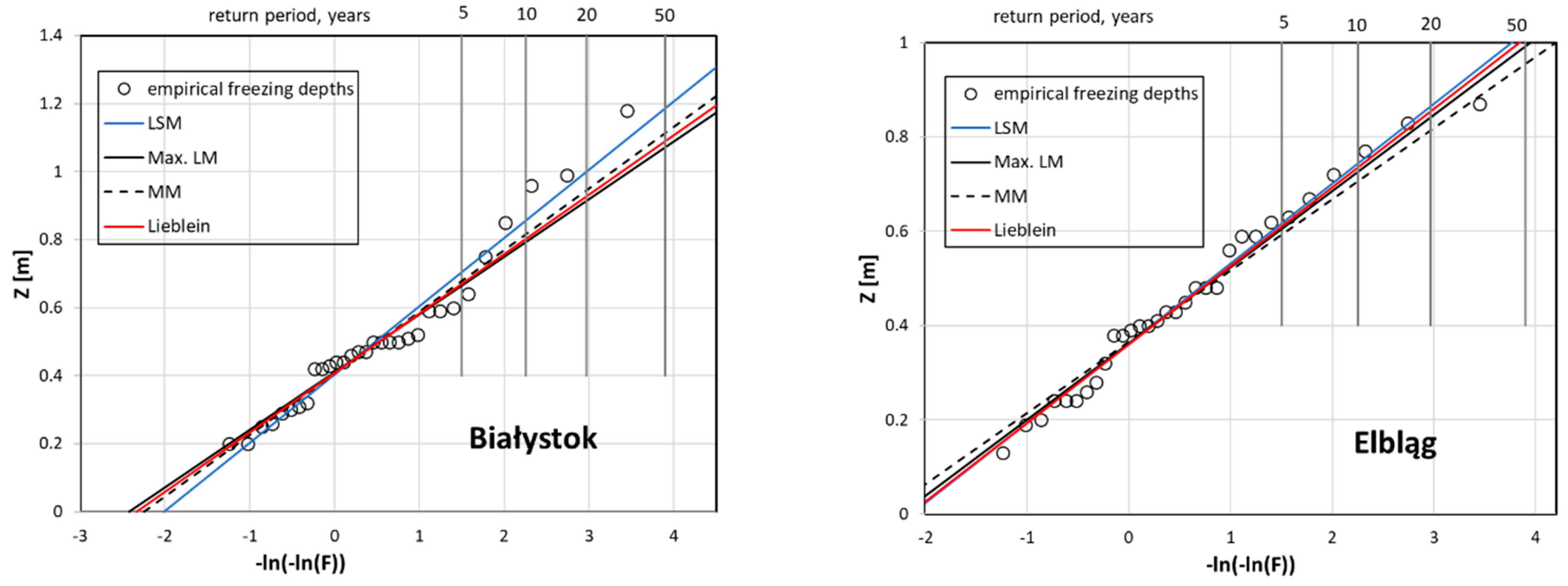
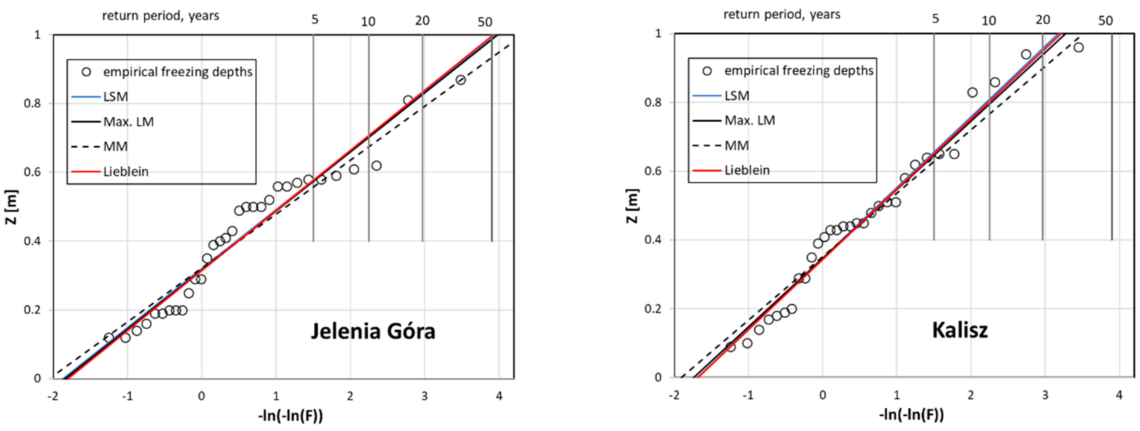
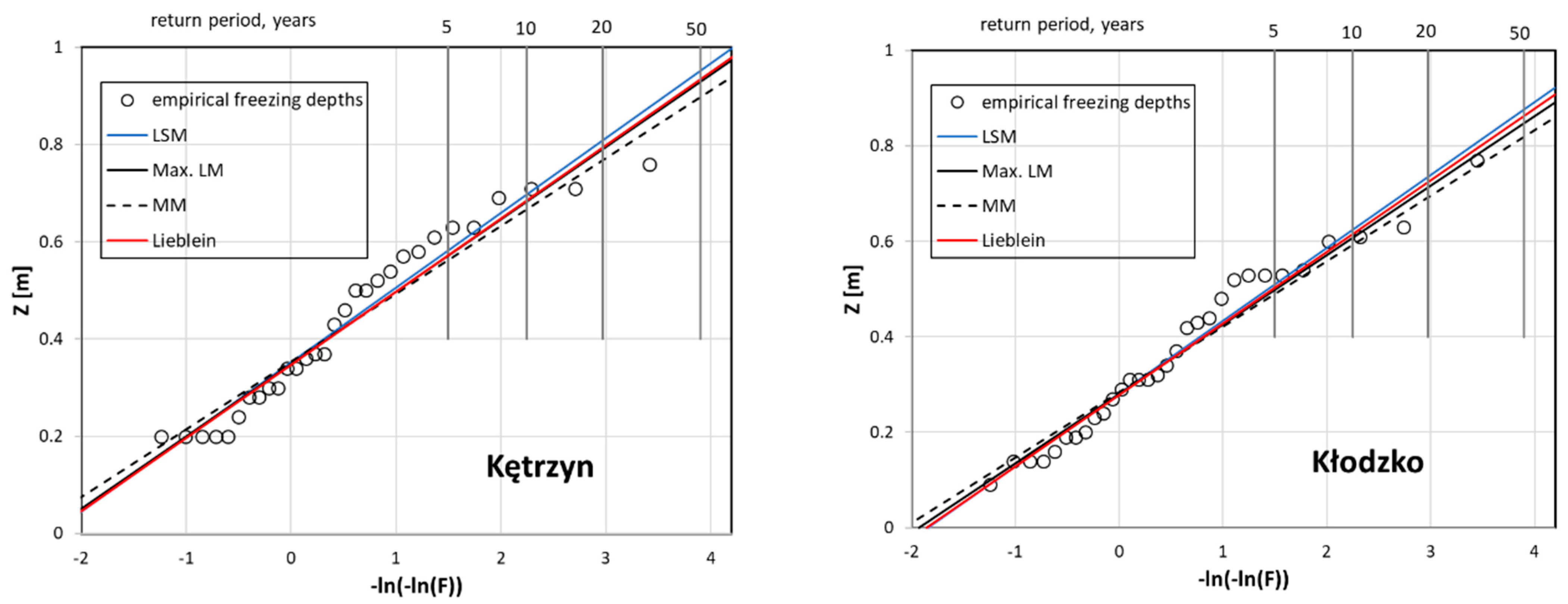
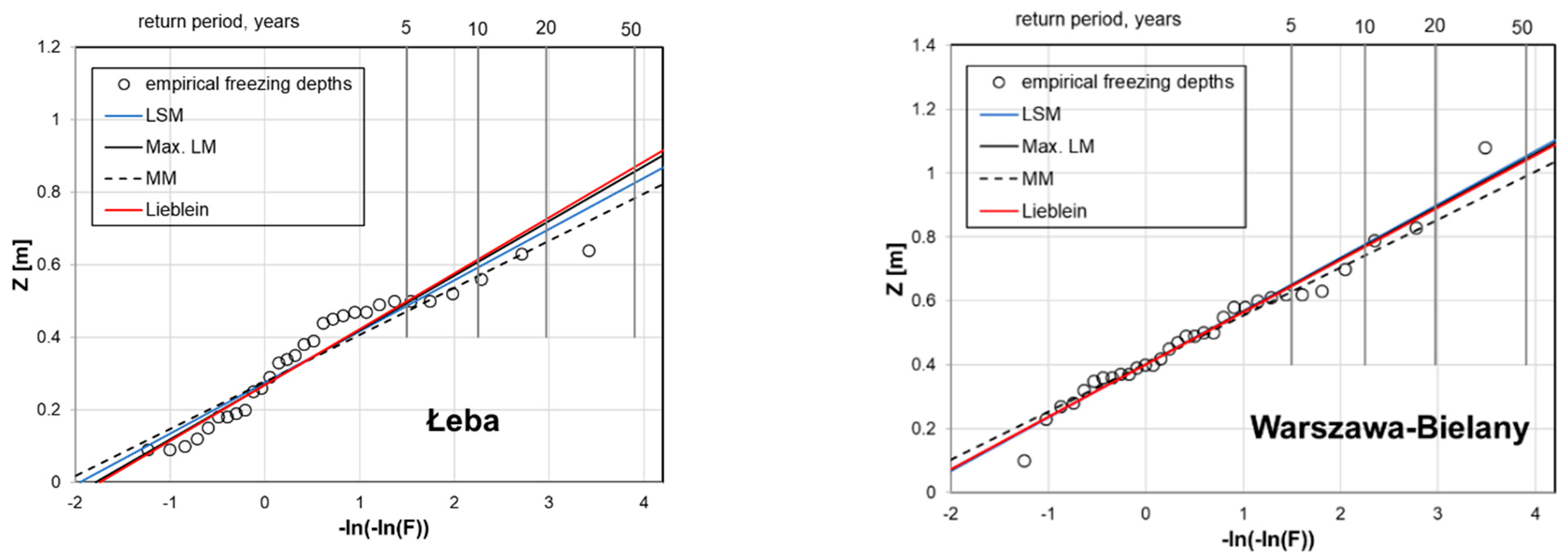
3.1. Estimation Models

From all recorded values of the position of zero centigrade temperature from measurements during every winter, one can extract the maximum depth and use in probabilistic calculations. Using the above mentioned Gumbel distribution, its parameters were estimated and the values of the predicted position of the zero isotherm in the ground were calculated (Figure 3, Figure 4, Figure 5 and Figure 6). Calculations were made for data from years 1980–2011.

This results in the location of the zero isotherm for the ground conditions of the 36 weather stations (first approach) where the measurements were made—

Table 1. Results of calculation for all localizations.

No.	Localization	Gumbel Distribution Parameters for Chosen Estimation Models:								Correlation Coefficient R2 for Lieblein
		LSM		Max. LM		MM		Lieblein
		α	u	α	u	α	u	α	U
1.	Białystok	4.980	0.404	5.895	0.410	5.515	0.407	5.717	0.408	0.980
2.	Bielsko-Biała	8.958	0.212	10.479	0.214	10.019	0.214	10.133	0.213	0.984
3.	Chojnice	4.460	0.400	5.334	0.407	5.005	0.405	5.130	0.404	0.990
4.	Elbląg	5.902	0.363	6.182	0.362	6.617	0.366	5.999	0.360	0.992
5.	Gorzów	4.664	0.302	5.647	0.307	5.150	0.305	5.555	0.306	0.977
6.	Jelenia Góra	5.831	0.320	5.826	0.316	6.385	0.322	5.733	0.315	0.971
7.	Kalisz	4.864	0.347	5.014	0.346	5.419	0.351	4.894	0.343	0.985
8.	Katowice	7.291	0.201	8.759	0.204	8.199	0.204	8.584	0.203	0.986
9.	Kętrzyn	6.506	0.352	6.726	0.349	7.178	0.354	6.643	0.347	0.973
10.	Kielce	4.645	0.399	5.351	0.404	5.157	0.402	5.191	0.402	0.979
11.	Kłodzko	6.541	0.281	6.865	0.280	7.284	0.284	6.663	0.278	0.985
12.	Koło	5.973	0.336	5.809	0.334	6.658	0.339	5.687	0.332	0.983
13.	Koszalin	6.065	0.313	6.669	0.316	6.817	0.317	6.449	0.313	0.991
14.	Kraków-Balice	6.670	0.261	6.721	0.258	7.328	0.263	6.565	0.256	0.972
15.	Łeba	7.097	0.275	6.643	0.268	7.709	0.276	6.498	0.268	0.958
16.	Legnica	4.592	0.327	4.952	0.328	5.136	0.332	4.790	0.325	0.987
17.	Lesko	7.026	0.234	8.079	0.237	7.875	0.237	7.897	0.235	0.986
18.	Leszno	5.208	0.350	5.459	0.349	5.826	0.354	5.294	0.347	0.992
19.	Lublin	5.682	0.333	6.244	0.335	6.364	0.337	6.099	0.332	0.991
20.	Łódź	4.699	0.386	4.905	0.386	5.284	0.391	4.736	0.382	0.992
21.	Mikołajki	6.024	0.311	6.656	0.312	6.718	0.315	6.510	0.311	0.986
22.	Nowy Sącz	8.851	0.202	8.788	0.199	9.776	0.203	8.526	0.198	0.977
23.	Opole	5.006	0.324	5.689	0.327	5.607	0.328	5.475	0.325	0.988
24.	Resko	5.888	0.245	6.623	0.247	6.539	0.248	6.537	0.246	0.982
25.	Rzeszów	8.658	0.351	7.514	0.344	9.415	0.351	7.498	0.344	0.959
26.	Sandomierz	5.560	0.434	6.095	0.436	6.141	0.436	6.014	0.434	0.974
27.	Słubice	5.857	0.298	6.476	0.300	6.544	0.301	6.290	0.297	0.991
28.	Suwałki	6.276	0.442	6.343	0.441	6.969	0.445	6.236	0.439	0.982
29.	Świnoujście	5.232	0.433	5.322	0.432	5.860	0.437	5.205	0.429	0.988
30.	Szczecin	4.253	0.282	4.616	0.279	4.622	0.284	4.633	0.280	0.961
31.	Tarnów	6.189	0.322	6.494	0.321	6.884	0.325	6.323	0.319	0.984
32.	Toruń	4.528	0.446	5.095	0.450	5.079	0.450	4.978	0.447	0.989
33.	Warszawa	5.986	0.401	6.066	0.402	6.647	0.404	6.109	0.401	0.985
34.	Włodawa	3.726	0.507	4.476	0.515	4.188	0.513	4.334	0.512	0.992
35.	Zakopane	5.450	0.378	5.050	0.372	6.008	0.380	4.998	0.370	0.975
36.	Zielona Góra	3.553	0.421	3.589	0.416	3.915	0.425	3.516	0.413	0.972

.

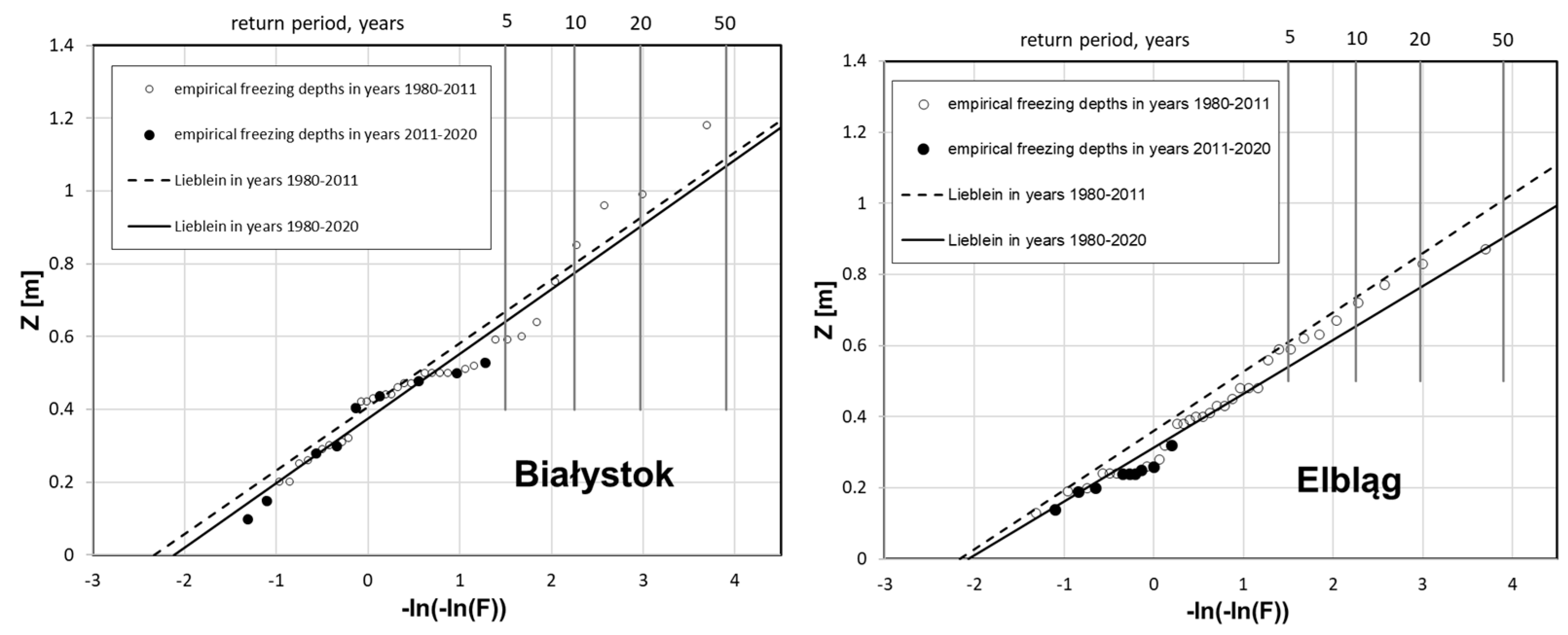
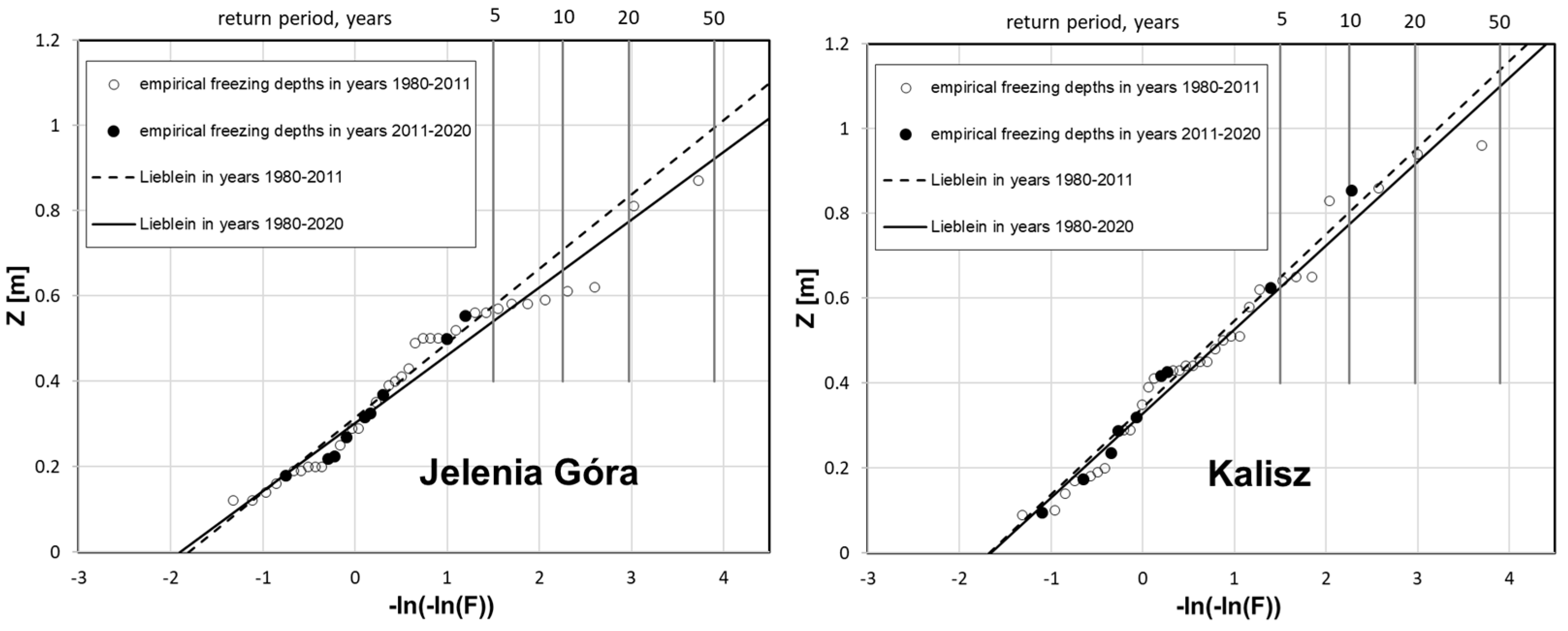
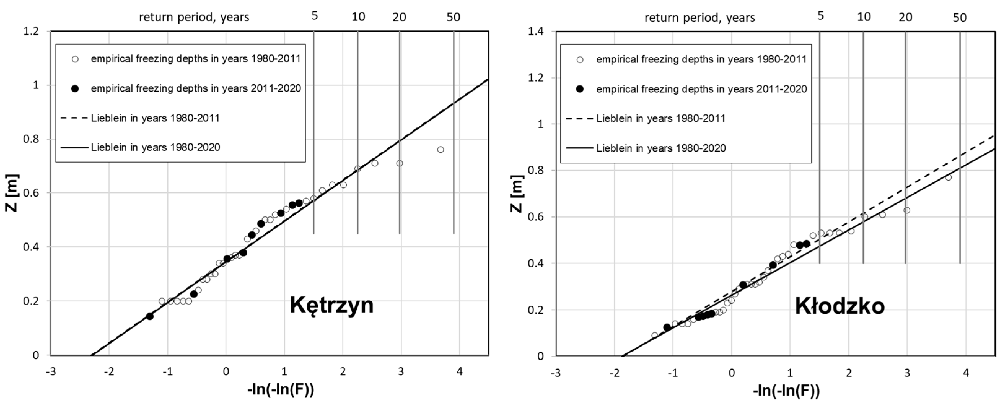
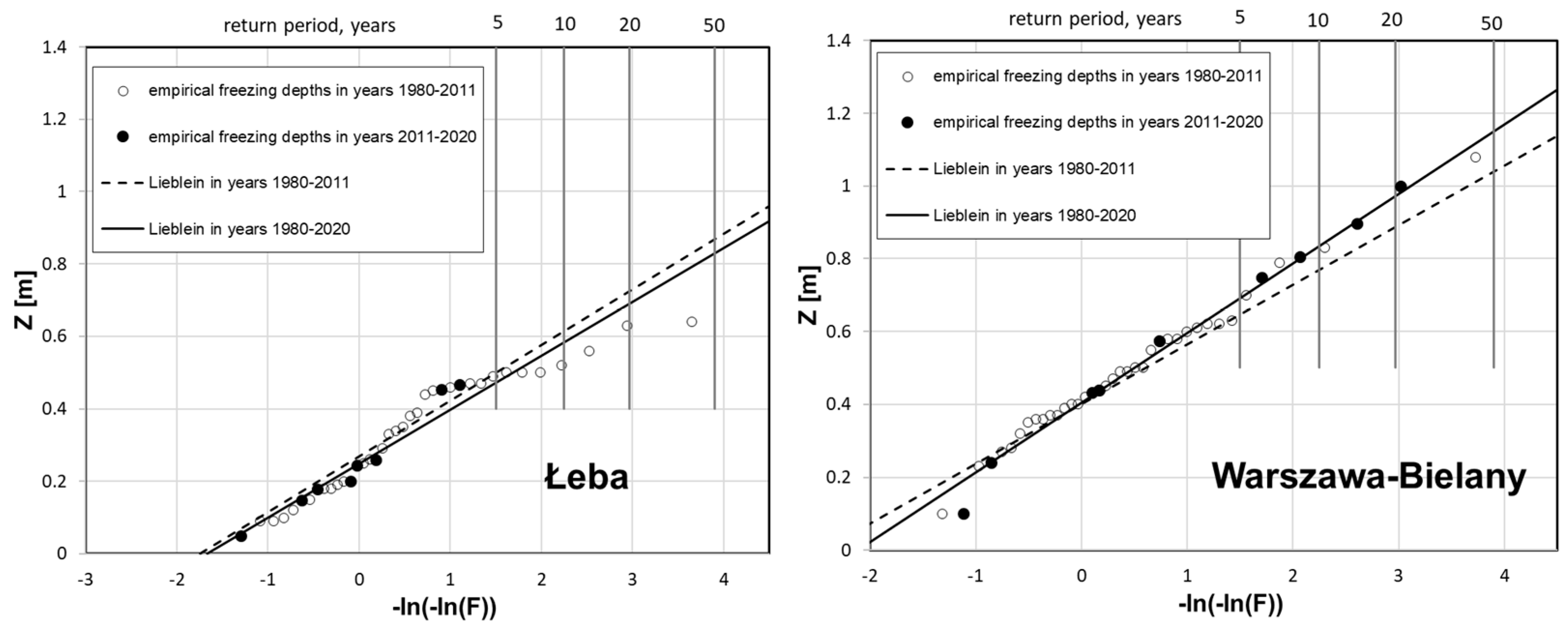
3.2. Validation of Chosen Model of Estimation (Lieblein)

It was assumed that, as in the case of climatic interactions, the characteristic values of the zero isotherm position should have a return period of 50 years—as required reference level to ensure the reliability in design.

For the next step of calculation, only one model of Gumbel’s method of analysis was used, with Lieblein’s best linear unbiased estimators (BLUE). These estimators are recommended in European Standard for climate actions, e.g., derivation of wind speeds from measurements at meteorological stations. To assess the correctness of the predictions indicated in the first approach, a recalculation was performed for the enlarged dataset. The new data related to freezing depth measurements, obtained from 2011 to 2020 (black points on graphs), were added. On this basis, the previous forecasts have been compared with the values based on current observations (Figure 7, Figure 8, Figure 9 and Figure 10). A new trendline has been set for the new data (1980–2020). With regard to the previous prediction, the change in the empirically determined freezing depth for the assumed return period (50 years) can thus be assessed.

4. Discussion and Conclusions

The use of the described method allows for a safe and reliable prediction of the depth of freezing of the ground. Real measurements over many years and an analysis of trends show that these values are not constant and subject to change. This is mainly due to the increasingly intense climate change associated with global warming. For the chosen locations, new predictions show that the empirical depth of freezing is general descending. This is one symptom of global warming.

The presented method of analyzing the depth of soil freezing takes into account actual soil temperature as a function of all external climatic actions with their coincidence and duration: air temperature, snow cover and precipitations. For this reason, it is more precise than the method using the so called air freezing index [16,26].

A comparison of calculation results related to the location of zero isotherm, conducted based on ground temperature analysis and freezing index (according to Gontaszewska [1]) leads to a conclusion that the second method has a lower accuracy. It does not account for snow cover, leading to much deeper freezing depths. Only in two cases (Leszno, Koszalin), almost the same results (difference of <2%) were obtained. The largest differences occurred in the mountains, where snowfall is the biggest (Jelenia Góra and Zakopane; values based on AFI are larger by 86%) and in North-East Poland (Białystok, 48%). Significant differences were also obtained in Warsaw (difference of 49%) and Kraków (77%).

Moreover, the probabilistic approach permits us to analyze the soil freezing in the terms of the reliability of structures. As the influence of climate can be easily analyzed using probabilistic approach, the influence of soil structure on the depth of freezing is much more complicated. It is due to the heterogeneity of soil and its structure. The depth of freezing is influenced by the type of the soil, its state of saturation, porosity, and mineral composition, and the arrangement of layers (Xu et al. [32], Żurawski & Godlewski [33], Yu, et al. [30]). This problem can be solved now only on the basis of the available literature using correction coefficients. One of the sources is available to authors now: former Soviet correction coefficients to the Formula (1) (Ickiewicz, Pogorzelski [34]): 23 for clays and silts, 28 for clay-sands, dusts and fine-grained sands, 30 for coarse-grained sands, and 34 for gravels. On the base of these values, it is possible to assume that gravel is a reference soil and the ratio of above mentioned values to 34 will be correction coefficients. In order to reduce the values based on different types of soil the inverse values of these coefficients will be used. An example is given below.

At Suwałki meteorological station the soil can be classified as silts and sands. In this case the actual depth of freezing reduced to the gravels as a standard reference soil can be received as a product of the calculated value 1.05 m for the 50-year return period and a factor of 34/28 = 1.21. If the soil in Suwałki region is assumed as a reference gravel, then the freezing depths will be 1.05 × 1.21 = 1.27 m. On the contrary, if we want to calculate the depth for clays and foams, we will receive 1.27 × (23/34) = 0.86 m.

Also, the lack of snow cover under conditions of reduced temperature can significantly increase the freezing range. Snow cover greatly inhibits freezing depths in soils, such that freezing depths can vary from year-to-year or spatially within a given time period, solely dependent on the presence or absence of a snow cover. The implications of a future climate, without or an increasingly intermittent snow cover, are greater freezing depths or varying depths, respectively. The currently observed snowless winters (in Poland and central part of Europe), with low rainfall (hydrological drought) and possible sudden waves of frost can lead to an increase in the range of freezing of the ground, which is already observed in the results of measurements and presented predictions.

At present, new analysis is currently being done in order to update the old provisions presented in Polish Standards. The influence of the soil structure will be taken into account using correction coefficients, as listed above. It should be noted here that the new prediction ranges and the depths of the zero isotherm are to be considered as design values representative for reliability analysis for the return period of 50 years.

Further research on the influence of the soil structure on its freezing is necessary. Such investigations should be carried out for different types of soil. They should also examine the difference between the depth of the position of zero centigrade temperature and actual frost penetration into the soil. Meanwhile, the correction coefficients will be used as presented above.

References

1. Gontaszewska, A. Thermophisical Properties in Soils in the Freezing Aspects; Uniwersytet Zielonogórski: Zielona Góra, Poland, 2010. (In Polish) [Google Scholar]
2. Konrad, J.-M.; Shen, M. 2-D frost action modeling using the segregation potential of soils. Cold Reg. Sci. Technol. 1996, 24, 263–278. [Google Scholar] [CrossRef]
3. Rajaei, P.; Baladi, G.Y. Frost Depth: General Prediction Model, Transportation Research Record. J. Transp. Res. Board 2015, 2510, 74–80. [Google Scholar] [CrossRef]
4. Venäläinen, A.; Tuomenvirta, H.; Heikinheimo, M.; Kellomäki, S.; Peltola, H.; Strandman, H.; Väisänen, H. Impact of climate change on soil frost under snow cover in a forested landscape. Clim. Res. 2001, 17, 63–72. [Google Scholar] [CrossRef] [Green Version]
5. Arctic and Subarctic Construction Calculation Methods for Determination of Depths of freeze and Thaw in Soils; Technical Manual: TM5-852-6/AFM; Departments of the Army and the Air Force: Washington, DC, USA, 1966.
6. Aldrich, H.P., Jr.; Paynter, H.M. Analytical Studies of Freezing and Thawing of Soils; First Interim Report; U.S. Army Corps of Engineeris, Airfields Branch, Engineering Division, Military Construction, ACFEL TR42: Boston, MA, USA, 1953. [Google Scholar]
7. Kersten, M.S. Thermal properties of soils. In Proceedings of the 30th Annual Meeting of the Highway Research Board, Highway Research Board Special Report: Frost Action in Soils: A Symposium, Washington, DC, USA, 9–12 January 1951; Volume 2, pp. 161–166. [Google Scholar]
8. Edwards, A.C.; Cresser, M.S. Freezing and its Effects on Chemical and Biological Properties of Soil. Adv. Soil Sci. 1992, 18, 59–79. [Google Scholar]
9. Wiłun, Z.; Piasecki, A.; Kowalewski, Z. Freezing of soils (Przemarzanie gruntów). In Informator Instytutu Technicznego Wojsk Lotniczych; Seria A, Nr 5/1962: Warsaw, Poland, 1962. (In Polish) [Google Scholar]
10. Zavarina, M.V. Methods of Computing Maximum Soil Freezing Depth; Translated from Voyeykov Main Geophysical Observatory (Trudy GGO). Sov. Hydrol. Sel. Papers 1969, 2, 131–139. [Google Scholar]
11. Nixon, J.F. Discrete ice lens theory for frost heave in soils. Can. Geotech. J. 1991, 28, 843–859. [Google Scholar] [CrossRef]
12. Tarnawski, V.R.; Wagner, B. On the prediction of hydraulic conductivity of frozen soils. Can. Geotech. J. 1996, 33, 176–180. [Google Scholar] [CrossRef]
13. Vermette, S.; Christopher, S. Using the rate of accumulated freezing and thawing degree days as a surrogate for determining freezing depth in a temperate forest soil. Middle States Geogr. 2008, 41, 68–73. [Google Scholar]
14. Goodrich, L.E. The Influence of Snow Cover on the Ground Thermal Regime. Can. Geotech. J. 1982, 19, 421–432. [Google Scholar] [CrossRef] [Green Version]
15. Grodecki, W. Analysis of Certain Real-World Ground Freezing Factors. Ph.D. Thesis, Politechnika Warszawska, Warszawa, Poland, 1971. (In Polish). [Google Scholar]
16. Gontaszewska, A. Comparison of calculated and observed depth of frost penetration in west Poland. In Faculty of Civil and Environmental Engineering, Institute of Structural Engineers; ASCE: New York, NY, USA, 2003. [Google Scholar]
17. Steurer, P.M. Probability distributions used in 100-year return period of air-freezing index. J. Cold Reg. Eng. 1996, 10, 25–35. [Google Scholar] [CrossRef]
18. Mageau, D.W.; Morgenstern, N.R. Observations on moisture migration in frozen soils. Can. Geotech. J. 1980, 17, 54–60. [Google Scholar] [CrossRef]
19. Żurański, J.A.; Sobolewski, A. About measurements of the soil temperature and forecasting of the depth of soil freezing. Inżynieria Bud. 2013, 3, 141–145. [Google Scholar]
20. Janiszewski, F. Instruction for Meteorological Stations; IMGW, Wydawnictwa Geologiczne: Warszawa, Poland, 1988. (In Polish) [Google Scholar]
21. World Meteorological Organization. Guide to Meteorological Instruments and Methods of Observation, WMO-No. 8; WMO: Geneva, Switzerland, 2018. [Google Scholar]
22. Gumbel, E.J. Statistics of Extremes; Columbia University Press: New York, NY, USA, 1958. [Google Scholar]
23. Żurański, J.A.; Sobolewski, A. Snow Loads in Poland (Obciążenie Sniegiem w Polsce); Instytut Techniki Budowlanej, Monografie: Warszawa, Poland, 2009. [Google Scholar]
24. Smith, M.G.; Rager, R.E. Protective Layer Design in Landfill Covers based on Frost Penetration. J. Geotech. Geoenviron. Eng. 2002, 128, 794–799. [Google Scholar] [CrossRef]
25. Lieblein, J. Efficient Methods of Extreme-Value Methodology; Technical Report, Institute for Applied Technology, National Bureau of Standards: WaWashington, DC, USA, 1976. [Google Scholar]
26. Żurawski, J.A.; Godlewski, T. Seasonal Ground Freezing in Poland; Instytut Techniki Budowlanej, Monografie: Warszawa, Poland, 2017. [Google Scholar]
27. Jakubek, M. Statistica (in Polish). Politechnika Krakowska, Poland. 2017. Available online: https://www.l5.pk.edu.pl/~mj/lib/exe/fetch.php?media=pl:dydaktyka:matematyka2:skrypt_statystyka.pdf (accessed on 5 April 2017).
28. Kozłowski, E. Mathematical Statistics. Lecture II: Point Estimation; Politechnika Lubelska: Lublin, Poland, 2020; Available online: http://www.kozlowski.pollub.pl/wyklady/SM/sm_wyklad2.pdf (accessed on 1 February 2020).
29. Plucińska, A.; Pluciński, E. Introduction to the Probability and Mathematical Statistics Account; Wydawnictwa Politechniki Warszawskiej: Warsaw, Poland, 1974. (In Polish) [Google Scholar]
30. Kordecki, W. Probability Account and Mathematical Statistics: Definitions, Theorems, Formulae; Oficyna Wydawnicza GiS: Wrocław, Poland, 2003. (In Polish) [Google Scholar]
31. Pekasiewicz, D. Selected compliance tests for extreme statistics distributions and their use in financial analysis. Pr. Nauk. Uniw. Ekon. Wrocławiu 2014, 371, 268–276. [Google Scholar] [CrossRef]
32. Xu, X.Z.; Wang, J.C.; Zhang, L.X. Physics of Frozen Soil; Science Press: Beijing, China, 2001. [Google Scholar]
33. Yu, F.; Guo, P.; Yuanming, L.; Stolle, D. Frost heave and thaw consolidation modelling. Part 1: A water flux function for frost heaving. Can. Geotech. J. 2020, 57, 1581–1594. [Google Scholar] [CrossRef]
34. Ickiewicz, I.; Pogorzelski, J.A. Influence of selected factors on the freezing depts in soils. Inżynieria Bud. 1987, 10–11, 338–342. [Google Scholar]
Figure 1. Example of temperature of the soil at the meteorological station in Białystok for one day (15 March 2005) adapted from [19].
Applsci 11 08194 g001
Figure 2. Example of extrapolation of the data on the soil temperature made in order to define maximal winter value adapted from [19].
Applsci 11 08194 g002
Figure 3. Estimation models for results from Białystok (left) and Elbląg (right) station—predicted position of zero isotherm for return period.
Applsci 11 08194 g003
Figure 4. Estimation models for results from Jelenia Góra (left) and Kalisz (right) station—predicted position of zero isotherm for return period.
Applsci 11 08194 g004
Figure 5. Estimation models for results from Kętrzyn (left) and Kłodzko (right) station—predicted position of zero isotherm for return period.
Applsci 11 08194 g005
Figure 6. Estimation models for results from Łeba (left) and Warszawa-Bielany (right) station—predicted position of zero isotherm for return period.
Applsci 11 08194 g006
Figure 7. Comparison of predicted and measurement value for chosen location: Białystok (left) and Elbląg (right) station.
Applsci 11 08194 g007
Figure 8. Comparison of predicted and measurement value for chosen location: Jelenia Góra (left) and Kalisz (right) station.
Applsci 11 08194 g008
Figure 9. Comparison of predicted and measurement value for chosen location: Kętrzyn (left) and Kłodzko (right) station.
Applsci 11 08194 g009
Figure 10. Comparison of predicted and measurement value for chosen location: Łeba (left) and Warszawa-Bielany (right) station.
Applsci 11 08194 g010