Tracking Control of Autonomous Underwater Vehicles with Acoustic Localization and Extended Kalman Filter

Abstract

The absence of global positioning system (GPS) signals and the influence of ocean currents are two of the main challenges facing the autonomy of autonomous underwater vehicles (AUVs). This paper proposes an acoustic localization-based tracking control method for AUVs. Particularly, three buoys that emit acoustic signals periodically are deployed over the surface. Times of arrivals of these acoustic signals at the AUV are then obtained and used to calculate an estimated position of the AUV. Moreover, the uncertainties involved in the localization and ocean currents are handled together in the framework of the extended Kalman filter. To deal with system physical constraints, model predictive control relying on online repetitive optimizations is applied in the tracking controller design. Furthermore, due to the different sampling times between localization and control, the dead-reckoning technique is utilized considering detailed AUV dynamics. To avoid using the highly nonlinear and complicated AUV dynamics in the online optimizations, successive linearizations are employed to achieve a trade-off between computational complexity and control performance. Simulation results show that the proposed algorithms are effective and can achieve the AUV tracking control goals.

1. Introduction

Autonomous underwater vehicles (AUVs) have been widely used for various purposes, e.g., military, commercial, and marine scientific survey applications [1]. For different purposes and scenarios, the requirement for the localization and control accuracy of AUVs ranges from meters to hundreds of meters. Compared to manned underwater vehicles, AUVs have no human pilots on board and thus avoid being exposed to dull and dangerous underwater environments. Compared to the tethered unmanned underwater vehicles, i.e., remotely operated vehicles (ROVs) [2], AUVs are tether free and thus can reach wider ocean spaces without the technical issues brought by the tether cable. The perception–plan–action cycle [3] is achieved by AUVs without persistent human instructions in order to accomplish the programmed missions. However, in the underwater environment, the attenuation rate of the global positioning system (GPS) signals is high, which makes GPS not applicable. Moreover, the ubiquitous ocean currents pose great influences on the relatively slow-moving AUVs. These factors impede the realization of the autonomy of AUVs.

In general, there are two types of localization methods underwater, i.e., distance independent methods and distance dependent methods [4]. Distance independent methods estimate the positions of underwater targets based on the topology of several beacon nodes. The most commonly used distance dependent methods include received signal strength indicator, time difference of arrival (TDOA), and time of arrival (TOA). They differ in the distance calculation processes. Multipath and shadow fading effects are usually concerned with the received signal strength indicator method. TOA methods use fewer fixed nodes than TDOA methods and are easier for implementation. The widely used base line localization methods are developed from TOA methods [5]. In TOA, the target position can be directly calculated based on the triangulation principle [6]. TOA has the advantages of low computational complexity and low cost. However, precise synchronization in-between subsurface nodes is often required which is hardly available in ocean applications considering the cost and power constraints. Besides, measurement noises play an important role in the localization accuracy. Improvement techniques such as the least square method and Kalman filter [7] have been proposed to overcome this issue. An extended Kalman filter (EKF) is designed to handle the measurement noises for a GPS intelligent buoy (GIB)-like system in underwater target tracking [8]. Experimental results show that the trajectory of the underwater target can be recovered well with the EKF based approach.

Besides the localization issue, another difference between AUVs and ground or airborne robots is that the influence of the dense ocean current flow cannot be neglected [9]. Therefore, various regional ocean models that generate realistic ocean current fields have been developed and used for AUV simulations [10]. For AUVs that operate in coastal regions, considering the collision risks with ships and land, ref. [11] utilizes the probabilistic ocean current predictions in the path planning of AUVs to improve the safety and reliability with stochastic approaches. By modeling the ocean current as a vector valued function of space and time, the current flow field is described as an Eulerian map in [10]. The Eulerian map then provides inputs to a planning and control module to optimize metrics such as energy consumption and path lengths. Instead of using the predicted ocean current values, another approach is to treat ocean current as environmental disturbances directly. Soft sensors, i.e., “observers”, are designed in [9,12] to achieve integrated current estimation and AUV motion control performance. In [13], in order to compensate for the steady-state error caused by the presence of ocean current, an adaptive/integral proportional derivative controller is designed for AUVs. The integral action has also been commented in [14] and is demonstrated to be a useful technique to achieve zero steady-state errors for systems with disturbances. Moreover, Kalman filter or EKF [15,16] is also commonly used for filtering general disturbances and estimating the motion states of marine robots. The estimated states can then be used for controller design assuming the “separation” principle holds so that the controller and observer could be designed separately.

With the information on localization and ocean current, the controller computes the input to the AUV system so as to achieve certain tasks. The most widely implemented controller is proportional-integral-derivative (PID) [13] due to its simplicity. More recent PID variants are usually equipped with gain scheduling [17] or fuzzy logic [18] designs to deal with nonlinearities. Lyapunov-based techniques such as backstepping [19] and sliding mode control [20] are also frequently used in AUV control to handle nonlinearities and guarantee convergence. However, these methods are often associated with tedious tuning procedures, and the control performance differs when the environment, load, or tasks change. Besides, control metrics and system constraints cannot be handled. In addition to systematically handling system constraints and optimizing performance, model predictive control (MPC) is inherently robust to disturbances to a certain degree [21]. MPC is applied to the AUV docking scenario in [22]. In [23], a series of MPC controllers are proposed to the AUV path following problem, and closed-loop system stability is guaranteed theoretically. A sliding mode control, a filtered Smith predictor, and an MPC controller are integrated in [24] to deal with disturbances, dead time, and constraints, respectively. However, most of the control problems assume the availability of the localization information of AUV, which is not practical.

In this paper, we consider the localization and control problem of AUVs simultaneously. In the absence of GPS signals, an acoustic localization method based on three surface buoys is first proposed. The three buoys emit acoustic signals periodically from the surface. The different times of arrivals of these signals at the AUV can then determine an estimated position of the AUV upon the receiving of the third signal in a localization cycle. Regarding the noises in the estimated positions, the unavailability of the velocity states, and the uncertainties due to the ocean current, an EKF approach is proposed to provide an estimate of the system’s full state. With the estimated system states, MPC is applied to track a reference trajectory. System physical constraints and control performance are explicitly considered. Since the localization and control have different sampling times, the dead-reckoning technique is utilized with detailed AUV dynamics. In the MPC controller design, to relieve the possible computational burden, the AUV dynamics are simplified through successive linearizations. Briefly, this paper contributes to the state of the art in the following aspects:

• a novel integrated acoustic localization and predictive tracking control approach is proposed for AUVs;
• the uncertainties in localization and ocean currents are handled together systematically using EKF;
• the approach of successive linearizations is applied to AUVs for computational efficiency. Simulation results demonstrate the effectiveness of the proposed algorithms for AUVs.

The remainder of the paper is organized as follows. Section 2 presents the AUV dynamic model and the tracking control problem statement. Then in Section 3, the acoustic localization method is proposed. The tracking control based on successively linearized prediction models, state estimation with EKF and MPC are further proposed in Section 4. Section 5 presents simulation results and discussions, followed by concluding remarks and future research considerations in Section 6.

2. AUV Modeling and Problem Statements

This section first presents the AUV dynamic models for later controller design and simulations, and then defines the localization and control problem considered in this paper.

2.1. AUV Modeling

The AUV motions can be modeled by two sets of differential equations: kinematics and kinetics. Kinematics deal with the geometrical relationships of the AUV motion. Kinetics follow Newton’s second law and analyze how the forces and moments that are generated by the thrusters cause the motion. Notably, AUVs maneuvering underwater inevitably experience ocean currents that also influence the system motions.

The AUV model used in this paper is modified from the REMUS AUV introduced in [25] where the values of all the mechanical design, hydrostatic and hydrodynamic parameters of the system have been made public. For simplicity, assumptions are made for the considered AUV dynamics that

• the origin $O_{\mathrm{b}}$ of the body-fixed coordinate system $\left\{b\right\}$ coincides with the center of gravity of the AUV;
• the AUV moves at a constant depth which can be measured accurately with a pressure sensor;
• the AUV is port-starboard symmetric;
• the AUV center of buoyancy coincides with the center of gravity.

The 6 Degrees Of Freedom (6 DOFs) motions are reduced to the horizontal 3-DOF motions neglecting the roll, pitch, and heave dynamics, as shown in Figure 1. Then, the 3-DOF AUV dynamics considering the influences of ocean currents are modeled following the vectorial format [14]. For notational simplicity, time dependence for system states and control inputs are left out in this section:

$$\begin{array}{cc}\hfill \dot{\mathbf{\eta }}& =\mathit{R}\left(\psi \right)\mathbf{\nu },\hfill \end{array}$$

(1)

$$\begin{array}{cc}\hfill \dot{\mathbf{\nu }}& ={\left({\mathit{M}}_{\mathrm{RB}}+{\mathit{M}}_{\mathrm{A}}\right)}^{-1}(\mathbf{\tau }-({\mathit{D}}_L+{\mathit{D}}_{\mathrm{NL}}+{\mathit{C}}_{\mathrm{A}}){\mathbf{\nu }}_{\mathrm{r}}-{\mathit{C}}_{\mathrm{RB}}\mathbf{\nu }+{\mathit{M}}_{\mathrm{A}}r{\mathit{S}}^{\mathrm{T}}{\mathbf{\nu }}_{\mathrm{c}}),\hfill \end{array}$$

(2)

where $\mathbf{\eta }={\left[\begin{array}{ccc}x& y& \psi \end{array}\right]}^{\mathrm{T}}$ indicates the pose states in the inertial coordinate system $\left\{n\right\}$, and $\mathbf{\nu }={\left[\begin{array}{ccc}u& v& r\end{array}\right]}^{\mathrm{T}}$ indicates the velocity states in the body-fixed coordinate system $\left\{b\right\}$. The more precise definition of the body-fixed AUV velocity is the velocity of the point $O_b$ with respect to $\left\{n\right\}$ expressed in $\left\{b\right\}$. The ocean current velocity vector ${\mathbf{\nu }}_{\mathrm{c}}$ is also defined in the body-fixed coordinate system $\left\{b\right\}$, as to be specified later. The controlled forces and moments are $\mathbf{\tau }={\left[\begin{array}{ccc}\xi & Y_{uu\delta }{u}^2\delta & N_{uu\delta }{u}^2\delta \end{array}\right]}^{\mathrm{T}}$ where $\xi$ and $\delta$, i.e., the system inputs, are the propeller thrust and rudder angle, respectively, and $Y_{uu\delta }$ and $N_{uu\delta }$ are the corresponding hydrodynamic parameters. The rotation matrix $\mathit{R}\left(\psi \right)$ relates the motions in $\left\{n\right\}$ and $\left\{b\right\}$:

$$\mathit{R}\left(\psi \right)=\left[\begin{array}{ccc}cos\left(\psi \right)& -sin\left(\psi \right)& 0\\ sin\left(\psi \right)& cos\left(\psi \right)& 0\\ 0& 0& 1\end{array}\right],$$

where $\psi$ is the heading angle, and $\mathit{R}$ satisfies $\frac{\mathrm{d}}{\mathrm{d}t}\left\{\mathit{R}\left(\psi \right)\right\}=\dot{\psi }\mathit{R}\left(\psi \right)\mathit{S}$ with

$$\mathit{S}=\left[\begin{array}{ccc}0& -1& 0\\ 1& 0& 0\\ 0& 0& 0\end{array}\right].$$

In Equation (2)$,{\mathbf{\nu }}_{\mathrm{r}}=\mathbf{\nu }-{\mathbf{\nu }}_{\mathrm{c}}={\left[\begin{array}{ccc}{u}_{\mathrm{r}}& v_{\mathrm{r}}& r_{\mathrm{r}}\end{array}\right]}^{\mathrm{T}}$ is the relative velocity in $\left\{b\right\}$ between the AUV hull and the ocean current. For simplification, we consider constant irrotational ocean current which is denoted as $\mathit{b}={[V_{\mathrm{c}},{\beta }_{\mathrm{c}}]}^{\mathrm{T}}$ where $V_{\mathrm{c}}$ and ${\beta }_{\mathrm{c}}$ are the current speed and angle in the inertial coordinate system $\left\{n\right\}$, respectively. Therefore, ${\beta }_{\mathrm{c}}=0$ means that the direction of the ocean current is aligned with the $x_{\mathrm{n}}$ axis. Then

$${\mathbf{\nu }}_{\mathrm{c}}=\mathit{R}{\left(\psi \right)}^{\mathrm{T}}\left[\begin{array}{c}{V}_{\mathrm{c}}cos{\beta }_{\mathrm{c}}\\ V_{\mathrm{c}}sin{\beta }_{\mathrm{c}}\\ 0\end{array}\right].$$

(3)

Therefore,

$${\dot{\mathbf{\nu }}}_{\mathrm{r}}=\dot{\mathbf{\nu }}-r{\mathit{S}}^{\mathrm{T}}{\mathbf{\nu }}_{\mathrm{c}}.$$

Rigid-body and added mass matrices are indicated as ${\mathit{M}}_{\mathrm{RB}}\in {\mathcal{R}}^{3\times 3}$ and ${\mathit{M}}_{\mathrm{A}}\in {\mathcal{R}}^{3\times 3}$, respectively ${\mathit{M}}_{\mathrm{RB}}$ and ${\mathit{M}}_{\mathrm{A}}$ are given as constant matrices here, and the inverse ${\left({\mathit{M}}_{\mathrm{RB}}+{\mathit{M}}_{\mathrm{A}}\right)}^{-1}$ exists for the given matrices. Similarly, ${\mathit{C}}_{\mathrm{RB}}$ and ${\mathit{C}}_{\mathrm{A}}$ are the rigid-body and added Coriolis and centripetal matrices, respectively. The damping effects are modeled by a ${\mathit{D}}_L$ and a nonlinear part ${\mathit{D}}_{\mathrm{NL}}$. The added and damping matrices are due to the hydrodynamic effects of marine crafts moving in fluid. The detailed matrix forms and paramter values can be found in the Appendix A.

Physical limitations are imposed on AUV speeds, and propeller and rudder working ranges as:

$$\begin{array}{c}{u}_{\min }⩽u⩽u_{\max },\end{array}$$

(4)

$$\begin{array}{c}{\xi }_{\min }⩽\xi ⩽{\xi }_{\max },\end{array}$$

(5)

$$\begin{array}{c}{\delta }_{\min }⩽\delta ⩽{\delta }_{\max }.\end{array}$$

(6)

2.2. Problem Statement

The AUV is required to start from an origin and track a time parameterized path to arrive at the destination. In the specified origin-destination region where the AUV operates, the ocean current information, i.e., $V_{\mathrm{c}}$ and ${\beta }_{\mathrm{c}}$, usually can be either predicted by regional ocean models or roughly measured by the sensors carried with the AUV [10]. However, these predictions or measurements are not precise and are mostly stochastically uncertain. Therefore, we assume that the ocean current could in principle be obtained by predictions, but with small prediction biased errors ${\mathbf{ϵ}}_b$ and uncertainties following a normal distribution as, i.e., $\mathit{b}\sim N\left(\overline{\mathit{b}}+{\mathbf{ϵ}}_b,{\Sigma }_b\right)$ where $\overline{\mathit{b}}=[{\overline{V}}_{\mathrm{c}},{\overline{\beta }}_{\mathrm{c}}]$, and ${\overline{V}}_{\mathrm{c}}$, ${\overline{\beta }}_{\mathrm{c}}$ are the predicted mean current speed and angle in the inertial coordinate system, respectively; ${\Sigma }_b=\mathit{diag}\left([{\sigma }_V^2,{\sigma }_{\beta }^2]\right)$ is the corresponding covariance that reflect the prediction accuracy where $diag$ means diagonal matrices; ${\mathbf{ϵ}}_b=[{ϵ}_v,{ϵ}_{\beta }]$ with ${ϵ}_v$ and ${ϵ}_{\beta }$ are the corresponding prediction biased errors, respectively. Note that the biased errors are unknown in the design process, and are modeled only for simulation purposes. In the simulations, we will explore how the ocean current biased errors influence the AUV motions as well as the robustness to small magnitude biased errors due to the feedback from acoustic localization. Furthermore, $V_{\mathrm{c}}$ and ${\beta }_{\mathrm{c}}$ are assumed to be independent and identically distributed random variables.

For the controller design, full states need to be known precisely for feedback in general. However, the sensors such as GPS that are used for the state measurement of ground or airborne vehicles are not applicable in the underwater environment. Therefore, in the next section, we first propose a distance dependent localization method to “measure” the AUV position.

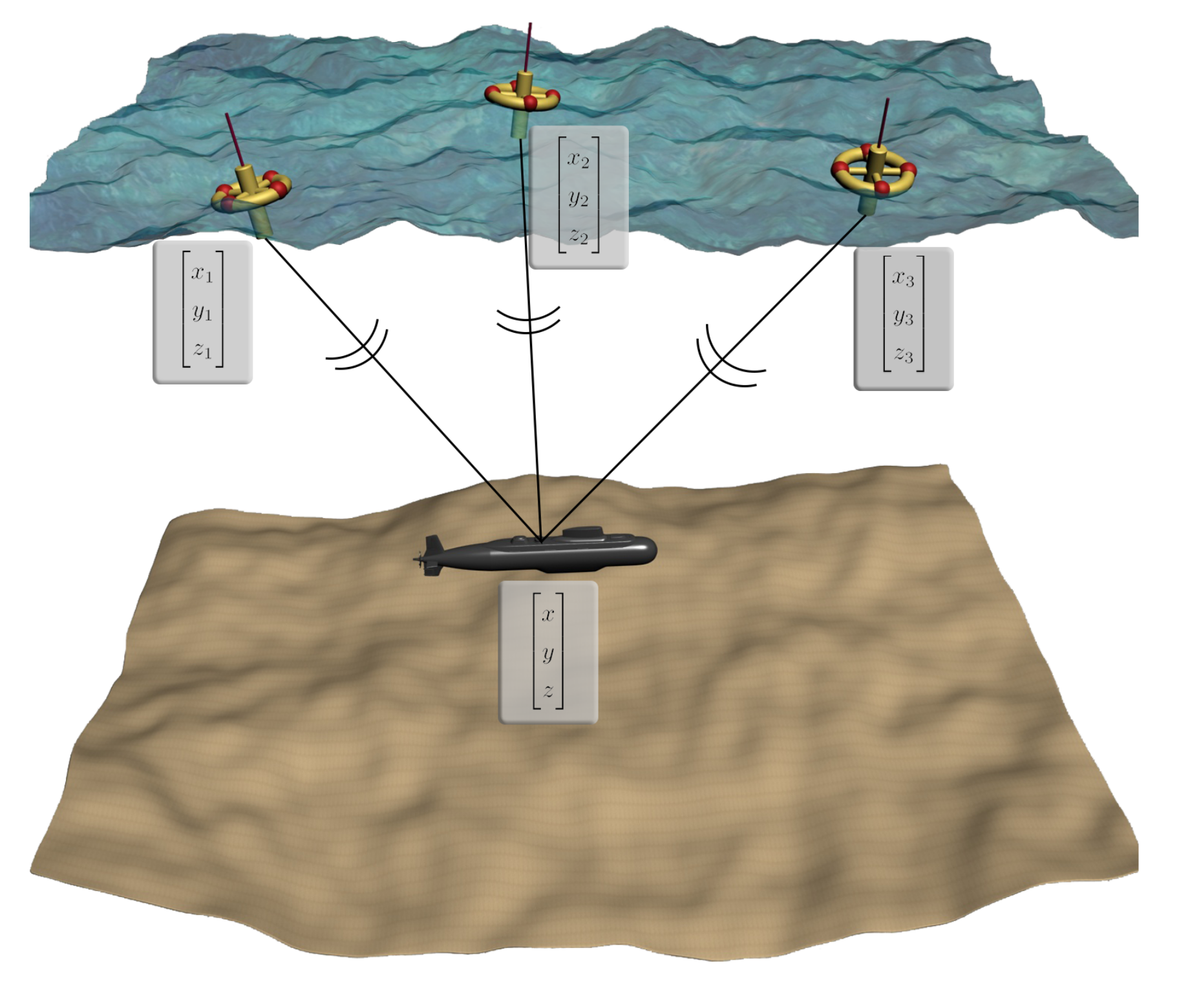
3. Acoustic Localization

Taking advantage of the finite propagation speed of sound in water and the availability of GPS or global navigation satellite system (GNSS) signals [26] over the ocean surface, we deploy three surface buoys with known positions ${[x_n,y_n,z_n]}^{\mathrm{T}}$, $n=1,2,3$, as shown in Figure 2. However, the underwater velocity of sound is generally not constant but varies with the water pressure, temperature, and conductivity. Therefore, the propagation path of the sound is actually curved, which leads to non-random deviations of signal arrival times. To overcome this difficulty, the ray tracing technique [27] with isogradient sound speed profiles (SSP) is utilized in the AUV acoustic localization problem.

Consider the scenario that each of the three buoys carries a pinger and emits acoustic signals every $T_s^l$ seconds. Denote the position of AUV as ${[x\left(t\right),y\left(t\right),z\left(t\right)]}^{\mathrm{T}}$ at time t. Since the depth of underwater vehicles can be accurately measured with a depth sensor [28], we consider the AUV to move at a known constant depth of z meters. The clocks of the three buoys and the AUV can be synchronized with either GPS or lower power atomic clocks. For the ray tracing problem between the surface buoys and the AUV, the SSP is dependent on the water depth as:

$$c=az+b$$

(7)

where c is the sound speed, a is a constant depending on the underwater environment, and b is the sound speed at the surface. Then, the TOAs of the signals from the three buoys at the AUV, denoted as $\Delta t_n$, $n=1,2,3$, can be calculated in simulations as [27]:

$$\begin{array}{cc}\hfill d_n\left(t\right)& =\sqrt{{(x\left(t\right)-x_n)}^2+{(y\left(t\right)-y_n)}^2}\hfill \end{array}$$

(8)

$$\begin{array}{cc}\hfill L_n& =\frac{0.5az}{b+0.5az}\hfill \end{array}$$

(9)

$$\begin{array}{cc}\hfill X_n\left(t\right)& =z/d_n\left(t\right)\hfill \end{array}$$

(10)

$$\begin{array}{cc}\hfill Y_n\left(t\right)& =L_n\left(t\right)/X_n\left(t\right)\hfill \end{array}$$

(11)

$$\begin{array}{cc}\hfill {\alpha }_n\left(t\right)& =arctan\left(Y_n\left(t\right)\right)\hfill \end{array}$$

(12)

$$\begin{array}{cc}\hfill {\beta }_n\left(t\right)& =arctan\left(X_n\left(t\right)\right)\hfill \end{array}$$

(13)

$$\begin{array}{cc}\hfill {\theta }_n^B\left(t\right)& ={\beta }_n\left(t\right)+{\alpha }_n\left(t\right)\hfill \end{array}$$

(14)

$$\begin{array}{cc}\hfill {\theta }_n^A\left(t\right)& ={\beta }_n\left(t\right)-{\alpha }_n\left(t\right)\hfill \end{array}$$

(15)

$$\begin{array}{cc}\hfill \Delta t_n\left(t\right)& =\frac{-1}{a}\left[ln\frac{1+sin{\theta }_n^A\left(t\right)}{cos{\theta }_n^A\left(t\right)}-ln\frac{1+sin{\theta }_n^B\left(t\right)}{cos{\theta }_n^B\left(t\right)}\right]\hfill \end{array}$$

(16)

where $d_n$ stands for the actual horizontal distance between buoy n and the AUV; $L_n$, $X_n$ and $Y_n$ are the intermediate variables; ${\alpha }_n$ is the angle between the actual sound ray and the straight line path for buoy n; ${\beta }_n$ is the angle between the horizontal direction and the straight line path for buoy n. Lastly, ${\theta }_n^B$ and ${\theta }_n^A$ are the grazing ray angles at buoy n and the AUV, respectively.

In simulations, TOAs $\Delta t_n\left(t\right)$, $n=1,2,3$ can be calculated as Equation (16), and in practice, they can be measured with synchronized clocks. Then, with the known TOAs, AUV depth z, and the fixed buoy locations, the horizontal distance ${\widehat{d}}_n$ could be estimated reversely using algorithms such as the binary search [27]. The main idea is to compare the arrival time of the median point with the actual propagation time repeatedly so that the search area could be narrowed down until a precise enough horizontal distance estimate ${\widehat{d}}_n$ is found.

Next, we are able to obtain the position of the AUV with ${\widehat{d}}_n$. If in one signal emit–receive cycle, the AUV is moving slowly and the position is assumed to be the same when the three signals from buoys 1, 2, and 3 are received, then we can get a set of nonlinear equations as:

$${(\widehat{x}\left(t\right)-x_n)}^2+{(\widehat{y}\left(t\right)-y_n)}^2={\widehat{d}}_n{\left(t\right)}^2,n=1,2,3,$$

(17)

by solving which we get the acoustically estimated position $\left(\widehat{x}\left(t\right),\widehat{y}\left(t\right)\right)$ of the AUV. Note that in practice, only two equations are necessary to be solved for $\left(\widehat{x}\left(t\right),\widehat{y}\left(t\right)\right)$. Available functions such as fsolve using trust-region algorithm in Matlab [29] can be applied to solve Equation (17).

If the AUV horizontal heading is measured by on board sensors such as the inertial measurement unit as $\widehat{\psi }\left(t\right)$, the AUV horizontal pose can be obtained as:

$$\widehat{\mathit{y}}\left(t\right)={[\widehat{x}\left(t\right),\widehat{y}\left(t\right),\widehat{\psi }\left(t\right)]}^{\mathrm{T}}$$

(18)

which can be seen as the “measured” system output. In the underwater environment, signal-to-noise ratio (SNR) is usually used to describe the quality of the received signals. High SNR of the received signals means more accurate TOAs, which leads to high localization accuracy. Therefore, due to the uncertainties in measured TOAs, the surface buoy positions ${[x_n,y_n,z_n]}^{\mathrm{T}}$, and the yaw angle measurement system, the “measured” AUV output $\widehat{\mathit{y}}\left(t\right)$ is assumed to be subject to random noises $\mathbf{\epsilon }\sim N\left(\mathbf{0},\Sigma \right)$ where $\mathbf{\epsilon }$ is an ${\mathcal{R}}^{3\times 1}$ vector, and the covariance $\Sigma =\mathit{diag}\left([{\sigma }_x^2,{\sigma }_y^2,{\sigma }_{\psi }^2]\right)$ with ${\sigma }_x$, ${\sigma }_y$, and ${\sigma }_{\psi }$ being the corresponding standard deviations.

4. Tracking Control Based on EKF

Considering the nonlinear uncertain AUV dynamics in Equations (1) and (2) with state feedback information from acoustic localization, we propose the trajectory tracking controller with MPC and EKF. MPC uses a system prediction model to obtain the system trajectory over a future finite time interval. Optimization problems are formulated based on the predicted trajectories and are solved repetitively online in a receding horizon way, and thus also called receding horizon control. To relieve the possible computational burden using Equations (1) and (2) as the prediction models, successive linearizations are applied in the framework of MPC. Moreover, an EKF approach is proposed to handle the uncertainties in the system and acoustic measurements. Corrected system state information is obtained and used in the predictive tracking controller design. During the control time steps when the updated localization information is not available, the dead-reckoning technique is utilized.

4.1. Successively Linearized Prediction Models

The highly nonlinear and uncertain AUV dynamics in Equations (1) and (2) render the online optimization based MPC control difficult. The conventional one step linearization approach was proposed for autonomous surface vessels in [30]. The computational time is shown to be much shorter than using the nonlinear prediction models directly. However, the one step linearized model could lead to large linearization errors over the whole prediction horizon and thus degrade the control performance. Therefore, the successive linearization approach proposed in [31] is applied to achieve a trade-off between computational complexity and control performance. The basic idea is to utilize the whole sequence of control inputs from a previous time step and pre-calculate a shifted system trajectory for linearizations over all prediction steps. For completeness while avoiding repetitions, we briefly describe the implemented successive linearization algorithm for the uncertain AUV dynamics.

Generalize the AUV dynamics Equations (1) and (2) as:

$$\dot{\mathit{x}}\left(t\right)=f(\mathit{x}\left(t\right),\mathit{u}\left(t\right),\mathit{b}\left(t\right)),$$

(19)

where $f:{\mathbb{R}}^6\times {\mathbb{R}}^2\times {\mathbb{R}}^2\to {\mathbb{R}}^6$ is a nonlinear smooth function; $\mathit{x}={[{\mathbf{\eta }}^{\mathrm{T}},{\mathbf{\nu }}^{\mathrm{T}}]}^{\mathrm{T}}$ is the system full state; $\mathit{u}={[\xi ,\delta ]}^{\mathrm{T}}\in {\mathbb{R}}^2$ is the control input vector; $\mathit{b}$ is defined as before. For numerical simulations, continuous time model Equation (19) is discretized with zero-order-hold assumption as:

$$\mathit{x}(k+1)=\mathit{x}\left(k\right)+{\int }_{k{\mathrm{T}}_s^c}^{(k+1){\mathrm{T}}_s^c}f\left(\mathit{x}\right(k),\mathit{u}(k),\mathit{b}(k\left)\right)\mathrm{d}t.$$

(20)

where time step k relates with the real time t as $t=k{T}_{\mathrm{s}}^{\mathrm{c}}$ with control sampling time $T_{\mathrm{s}}^{\mathrm{c}}$. Note that the control sampling time $T_{\mathrm{s}}^{\mathrm{c}}$ is not necessarily the same with the localization sampling time $T_{\mathrm{s}}^{\mathrm{l}}$. At each control time step k, successive linearizations are primarily implemented as:

• Shift the optimal control input sequence from the previous step, ${\mathit{u}}^{*}\left(i\right|k-1),i=0,1,\cdots ,N_{\mathrm{p}}-1$ with $N_{\mathrm{p}}$ being the discrete horizon steps, to obtain a seed control input trajectory ${\mathit{u}}^0\left(i\right|k)$:

  $${\mathit{u}}^0\left(i\right|k)={\mathit{u}}^{*}\left(i\right|k-1)$$

  for $i=0,1,\cdots ,N_{\mathrm{p}}-2$ and

  $${\mathit{u}}^0(N_{\mathrm{p}}-1|k)={\mathit{u}}^{*}(N_{\mathrm{p}}-2|k-1).$$
• Apply ${\mathit{u}}^0\left(i\right|k)$ to Equation (20) and obtain a seed state trajectory ${\mathit{x}}^0\left(i\right|k),i=0,1,\cdots ,N_{\mathrm{p}}$. The initial state is set as ${\mathit{x}}^0\left(0\right|k)=\mathit{x}\left(k\right)$ with $\mathit{x}\left(k\right)$ being the current system state. The seed disturbance values are set as

  $${\mathit{b}}^0\left(i\right|k)=\overline{\mathit{b}}\left(i\right|k),i=0,1,\cdots ,N_{\mathrm{p}}-1$$

  (21)

  where $\overline{\mathit{b}}\left(i\right|k)$ is constant as $[{\overline{V}}_{\mathrm{c}},{\overline{\beta }}_{\mathrm{c}}]$ for simplicity without loss of generality. The proposed algorithm is still applicable and works effectively when time-varying values for $[{\overline{V}}_{\mathrm{c}},{\overline{\beta }}_{\mathrm{c}}]$ are available. The EKF that will be introduced in the next subsection is also based on linearizations at the mean values of random disturbances.
• Linearize the nonlinear dynamics at the seed trajectories $\left({\mathit{x}}^0\left(i\right|k),{\mathit{u}}^0\left(i\right|k),{\mathit{b}}^0\left(i\right|k)\right)$ for $i=0,1,\cdots ,N_{\mathrm{p}}-1$ as:

  $$\mathit{x}(i+1|k)={\mathit{x}}^0(i+1|k)+\mathit{A}\left(i\right|k)\Delta \mathit{x}\left(i\right|k)+\mathit{B}\left(i\right|k)\Delta \mathit{u}\left(i\right|k)+\mathit{E}\left(i\right|k)\Delta \mathit{b}\left(i\right|k)$$

  (22)

  where

  $$\begin{array}{cc}\hfill \Delta \mathit{x}\left(i\right|k)& =\mathit{x}\left(i\right|k)-{\mathit{x}}^0\left(i\right|k)\hfill \end{array}$$

  (23)

  $$\begin{array}{cc}\hfill \Delta \mathit{u}\left(i\right|k)& =\mathit{u}\left(i\right|k)-{\mathit{u}}^0\left(i\right|k)\hfill \end{array}$$

  (24)

  $$\begin{array}{cc}\hfill \Delta \mathit{b}\left(i\right|k)& =\mathit{b}\left(i\right|k)-{\mathit{b}}^0\left(i\right|k)\hfill \end{array}$$

  (25)

  are small perturbations around ${\mathit{x}}^0\left(i\right|k)$, ${\mathit{u}}^0\left(i\right|k)$ and ${\mathit{b}}^0\left(i\right|k)$, respectively; $\mathit{A}\left(i\right|k)$, $\mathit{B}\left(i\right|k)$, and $\mathit{E}\left(i\right|k)$ are the corresponding Jacobian matrices, respectively, of the nonlinear dynamics function Equation (20) evaluated at $\left({\mathit{x}}^0\left(i\right|k),{\mathit{u}}^0\left(i\right|k),{\mathit{b}}^0\left(i\right|k)\right)$.

4.2. EKF with Acoustic Localization Information

Kalman filter is a widely used correct-predict formulation to deal with velocity estimation and stochastic environmental disturbances [15]. EKF further extends the system dynamics to nonlinear types by linearizations to propagate an approximation of the state estimation and covariance. With the models Equations (18), (20) and (22), we are ready for the EKF design.

Assuming that $T_{\mathrm{s}}^{\mathrm{l}}=n{T}_{\mathrm{s}}^{\mathrm{c}}$ and $n\ge 2$ is an integer. Then, at control time step k while the new acoustic localization information is available, i.e., the localization step $k/n$, the AUV predicted state is corrected by

$$\widehat{\mathit{x}}\left(k\right)=\overline{\mathit{x}}\left(k\right)+\mathit{K}\left(k\right)[\widehat{\mathit{y}}\left(k\right)-\mathit{C}\overline{\mathit{x}}\left(k\right)],$$

(26)

where

$$\mathit{C}=\left[\begin{array}{cccccc}1& 0& 0& 0& 0& 0\\ 0& 1& 0& 0& 0& 0\\ 0& 0& 1& 0& 0& 0\end{array}\right],$$

(27)

is the output matrix; $\overline{\mathit{x}}\left(k\right)$ is the predicted state by ignoring the uncertainties in the nonlinear dynamics Equation (20), i.e.,

$$\overline{\mathit{x}}(k+1)=f_{\mathrm{d}}(\overline{\mathit{x}}\left(k\right),\mathit{u}\left(k\right),\overline{\mathit{b}}\left(k\right)),$$

(28)

where $f_{\mathrm{d}}$ is the discrete function that generalizes Equation (20). Note the the parameters with a horizontal bar overhead such as $\overline{\mathit{b}}$ and $\overline{\mathit{x}}$ all indicate the predicted system information. The Kalman gain matrix $\mathit{K}\left(k\right)$ is derived by

$$\mathit{K}\left(k\right)=\left\{\begin{array}{cc}\overline{\mathit{P}}\left(k\right){\mathit{C}}^{\mathrm{T}}{\left(\mathit{C}\overline{\mathit{P}}\left(k\right){\mathit{C}}^{\mathrm{T}}+\Sigma \right)}^{-1},\hfill & \mathrm{if}k/n\mathrm{is}\mathrm{integer},\hfill \\ {[0,0,0]}^{\mathrm{T}},\hfill & \mathrm{otherwise}.\hfill \end{array}\right.$$

The covariance matrix $\overline{\mathit{P}}\left(k\right)$ for the prediction error $\mathit{x}\left(k\right)-\overline{\mathit{x}}\left(k\right)$ is computed by the recursion

$$\begin{array}{cc}\hfill \mathit{P}\left(k\right)& =\left(\mathit{I}-\mathit{K}\left(k\right)\mathit{C}\right)\overline{\mathit{P}}\left(k\right),\hfill \end{array}$$

(29)

$$\begin{array}{cc}\hfill \overline{\mathit{P}}(k+1)& =\mathit{A}\left(0\right|k)\mathit{P}\left(k\right){\mathit{A}}^{\mathrm{T}}\left(0\right|k)+\mathit{E}\left(0\right|k){\Sigma }_b{\mathit{E}}^{\mathrm{T}}\left(0\right|k),\hfill \end{array}$$

(30)

where $\mathit{P}\left(k\right)$ is the covariance matrix of the estimation error $\mathit{x}\left(k\right)-\widehat{\mathit{x}}\left(k\right)$.

Through this standard Kalman filter procedure, the predicted system state $\overline{\mathit{x}}\left(k\right)$ can be corrected by the acoustically “measured” outputs $\mathit{y}\left(k\right)$ whenever this information is available. The corrected states $\widehat{\mathit{x}}\left(k\right)$ can then be used for feedback design in MPC. However, as mentioned earlier, the control cycle is generally shorter than the localization cycle, i.e., $T_{\mathrm{s}}^{\mathrm{c}}\le T_{\mathrm{s}}^{\mathrm{l}}$, which means $\mathit{y}\left(k\right)$ is not guaranteed to be there for each control time step k. When the acoustic measurement is not available, the predicted state $\overline{\mathit{x}}\left(k\right)$ from Equation (28) is used for feedback, which is commonly known as the dead-reckoning technique [14].

4.3. Predictive Tracking Control

Briefly, at each time step k, MPC computes a future control sequence over the prediction horizon $N_{\mathrm{p}}$ based on the current system state. The predicted system trajectory is then driven close to the given reference. Only the first element of the control sequence is applied to the system. At the next time step $k+1$, this process is repeated over the shifted prediction horizon with newly measured system states. MPC is based on solving optimization problems online repetitively and mostly numerically, which naturally and explicitly handles system constraints. Therefore, MPC is especially suitable to systems of which analytical control laws are difficult to derive, and suitable to systems with constraints. For the AUV tracking problem, system constraints Equations (4)–(6) are imposed. We next propose the MPC approach to solve the AUV tracking problem with the corrected information from EKF or the predicted information from dead-reckoning.

Consider at time step k, given the current estimated $\overline{\mathit{x}}\left(k\right)$ when the acoustic estimated state $\widehat{\mathit{x}}\left(k\right)$ is not available, future predicted trajectories $\mathit{x}\left(i\right|k)$ over $N_{\mathrm{p}}$ are then made following Equation (22). Moreover, given a reference path determined by an origin $(x_{\mathrm{o}},y_{\mathrm{o}})$ and a destination $(x_{\mathrm{d}},y_{\mathrm{d}})$ in the inertial coordinate system, a constant reference speed $u_{\mathrm{d}}$ is set to parameterize path. The reference trajectory over a future prediction horizon $N_{\mathrm{p}}$ at k is calculated as

$${\mathit{y}}_{\mathrm{r}}\left(i\right|k)=\left[\begin{array}{c}{x}_{\mathrm{o}}\\ y_{\mathrm{o}}\\ {\psi }_{\mathrm{d}}\end{array}\right]+u_{\mathrm{d}}{T}_{\mathrm{s}}^{\mathrm{c}}(k+i)\left[\begin{array}{c}cos\left({\psi }_{\mathrm{d}}\right)\\ sin\left({\psi }_{\mathrm{d}}\right)\\ 0\end{array}\right],$$

(31)

where ${\psi }_{\mathrm{d}}=arctan\left(\left(y_{\mathrm{d}}-y_0\right)/\left(x_{\mathrm{d}}-x_0\right)\right)$. The tracking problem is then represented by solving a constrained finite horizon linear programming problem

$$\underset{\mathit{u}\left(i\right|k)}{min}\left|\right|\overline{\mathit{y}}\left(N_{\mathrm{p}}\right|k)-{\mathit{y}}_{\mathrm{r}}\left(N_{\mathrm{p}}\right|k){\left|\right|}_{{\mathit{Q}}_f}^2+\sum _{i=0}^{N_p-1}\left|\right|\overline{\mathit{y}}\left(i\right|k)-{\mathit{y}}_{\mathrm{r}}{\left(i\right|k)\left|\right|}_{\mathit{Q}}^2+{\left|\right|\mathit{u}\left(i\right|k)\left|\right|}_{\mathit{R}}^2,$$

(32)

subject to Equation (22) and

$$\begin{array}{cc}\hfill & \mathit{x}\left(0\right|k)=\widehat{\mathit{x}}\left(k\right)\mathrm{or}\overline{\mathit{x}}\left(k\right),\hfill \end{array}$$

(33)

$$\begin{array}{cc}\hfill u_{\min }& ⩽u\left(i\right|k)⩽u_{\max },i=0,1,\cdots ,N_{\mathrm{p}},\hfill \end{array}$$

(34)

$$\begin{array}{cc}\hfill {\xi }_{\min }& ⩽\xi \left(i\right|k)⩽{\xi }_{\max },i=0,1,\cdots ,N_{\mathrm{p}}-1,\hfill \end{array}$$

(35)

$$\begin{array}{cc}\hfill {\delta }_{\min }& ⩽\delta \left(i\right|k)⩽{\delta }_{\max },i=0,1,\cdots ,N_{\mathrm{p}}-1,\hfill \end{array}$$

(36)

where $\overline{\mathit{y}}\left(i\right|k)=\mathit{C}\overline{\mathit{x}}\left(i\right|k)$. The cost function Equation (32) aims to minimize the tracking error between the predicted state trajectory and the reference trajectory with optimal control efforts. The three terms are the terminal tracking error cost, the stage tracking error cost, and the control input cost, respectively; ${\mathit{Q}}_f$, $\mathit{Q}$ and $\mathit{R}$ are positive definite weighting matrices for the respective cost terms and can be adjusted to set priority between convergence speed and control efforts. Due to the constraints on system states and control inputs, the optimization problem does not have an analytical solution, and needs to be solved numerically repetitively online with newly “measured” system states and time-varying prediction models. However, due to the successive linearization, the above optimization problem becomes convex and can be solved efficiently.

Overall, the predictive tracking control algorithm with EKF and acoustic localization information or dead-reckoning can be summarized as Algorithm 1.

Algorithm 1 Predictive tracking control of AUV with acoustic localization and EKF

1: Initialize at $k=0$, set $\overline{\mathit{x}}\left(0\right)=\mathit{x}\left(0\right)$, $\widehat{\mathit{x}}\left(0\right)=\mathit{x}\left(0\right)$; 2: while The AUV has not arrived the destination do 3:   if Acoustic localization counter = n then 4:    Obtain $\widehat{\mathit{y}}\left(k\right)$ as in Section 3 5:    Calculate $\overline{\mathit{P}}\left(k\right)$ and $\mathit{K}\left(k\right)$; 6:    Correct $\overline{\mathit{x}}\left(k\right)$ with $\widehat{\mathit{y}}\left(k\right)$ and $\mathit{K}\left(k\right)$ as in (26); 7:    Update $\mathit{P}\left(k\right)$ 8:    counter→ 0 9:   else 10:    Update $\overline{\mathit{x}}\left(k\right)$ with dead-reckoning as in (28); 11:   end if 12:   Solve the optimization problem (32) subject to (22), (33)–(36) to obtain ${\mathit{u}}^{*}\left(k\right)$; 13:   Apply ${\mathit{u}}^{*}\left(k\right)$ to the AUV system (1) and (2); 14:   Set $k=k+1$, counter + 1 → counter and go to Step 3; 15: end while

5. Simulation Results and Discussions

Simulations are run to demonstrate the effectiveness of the proposed tracking control algorithms for AUVs. The proposed integrated localization and control algorithm is applied in following a reference path. Such applications can be seen in sea mapping scenarios where only waypoints in the concerned ocean region are given. The AUV is positioned at the initial point $[100,100,300]$ m and is controlled to reach the destination $[600,600,300]$ m along the following curved reference path

$$\left\{\begin{array}{cc}\hfill x_{\mathrm{d}}\left(t\right)& =600-500cos(\pi t/1200),\hfill \\ \hfill y_{\mathrm{d}}\left(t\right)& =100+500sin(\pi t/1200),\hfill \end{array}\right.$$

for $t\in [0,600]$ s. The three surface buoys are positioned at $[0,0,0]$ m, $[500,800,0]$ m, and $[1000,0,0]$ m, respectively. The isogradient SSP parameters in (7) are set as: $a=-0.05$ and $b=1540$ m/s. In this region, ocean currents exist. The average speed is predicted to be 0.5 m/s and the angle is predicted to be $\pi$/6. However, there might be prediction biased errors. In the simulations, we will first validate the performance of the proposed integrated localization and tracking control algorithm with zero prediction biased errors, i.e., ${ϵ}_v=0$ and ${ϵ}_{\beta }=0$. Then, to illustrate the inherent robustness (to a certain degree) of the feedback due to acoustic localization, we also consider non-zero prediction biased errors with ${ϵ}_v=0.15$ m/s and ${ϵ}_{\beta }=\pi /20$ rad. Note that the biased errors are not considered explicitly in the algorithm design, and are only implemented for simulation purposes to show the inherent robustness due to the feedback from the acoustic localization. Moreover, there exist uncertainties with the predicted values following the normal distribution with covariance ${\Sigma }_b=diag\left([0.1{\mathrm{m}}^2/{\mathrm{s}}^{2}0.01{\mathrm{rad}}^2]\right)$, which means low prediction accuracy in the ocean current. It should be noted that AUVs with any design may fail at those worst predictions of the sea. The uncertain acoustic measurement is with covariance $\Sigma =diag\left(\left[0.1{\mathrm{m}}^{2}0.1{\mathrm{m}}^{2}0.01{\mathrm{rad}}^2\right]\right)$. The AUV depth is 300 m, and the buoy depths are all 0 m. Controller parameters are set as follows: prediction horizon $N_{\mathrm{p}}=10$; weight parameter ${\mathit{Q}}_f=\mathit{Q}=diag\left(\left[100100\right]\right)$ and $\mathit{R}=diag\left(\right[1180/\pi \left]\right)$; sampling time $T_{\mathrm{s}}^{\mathrm{c}}=0.5$ s and $T_{\mathrm{s}}^{\mathrm{l}}=1$ s, which means the system feedback states are corrected by the acoustic localization results every two control time steps, i.e., n = 2 in Algorithm 1. Physical system constraints are: $u_{\max }=-u_{\min }=$ 2 m/s, ${\mathbf{\xi }}_{\max }=-{\mathbf{\xi }}_{\min }$ = 86 N, and ${\mathbf{\delta }}_{\max }=-{\mathbf{\delta }}_{\min }$ = 13.6$\pi /180$ rad. The REMUS AUV system parameter values are referred to [25]. Note that the practical parameter values might be different from the above set values. For adverse environmental situations, the algorithm might not be applicable. All the algorithms are implemented in MATLAB 2016b [29] with solver Cplex [32] on a platform with Intel(R) Core(TM) i3-7100 CPU @ 3.70 GHz.

5.1. Tracking Control with Acoustic Localization

5.1.1. Localization Results

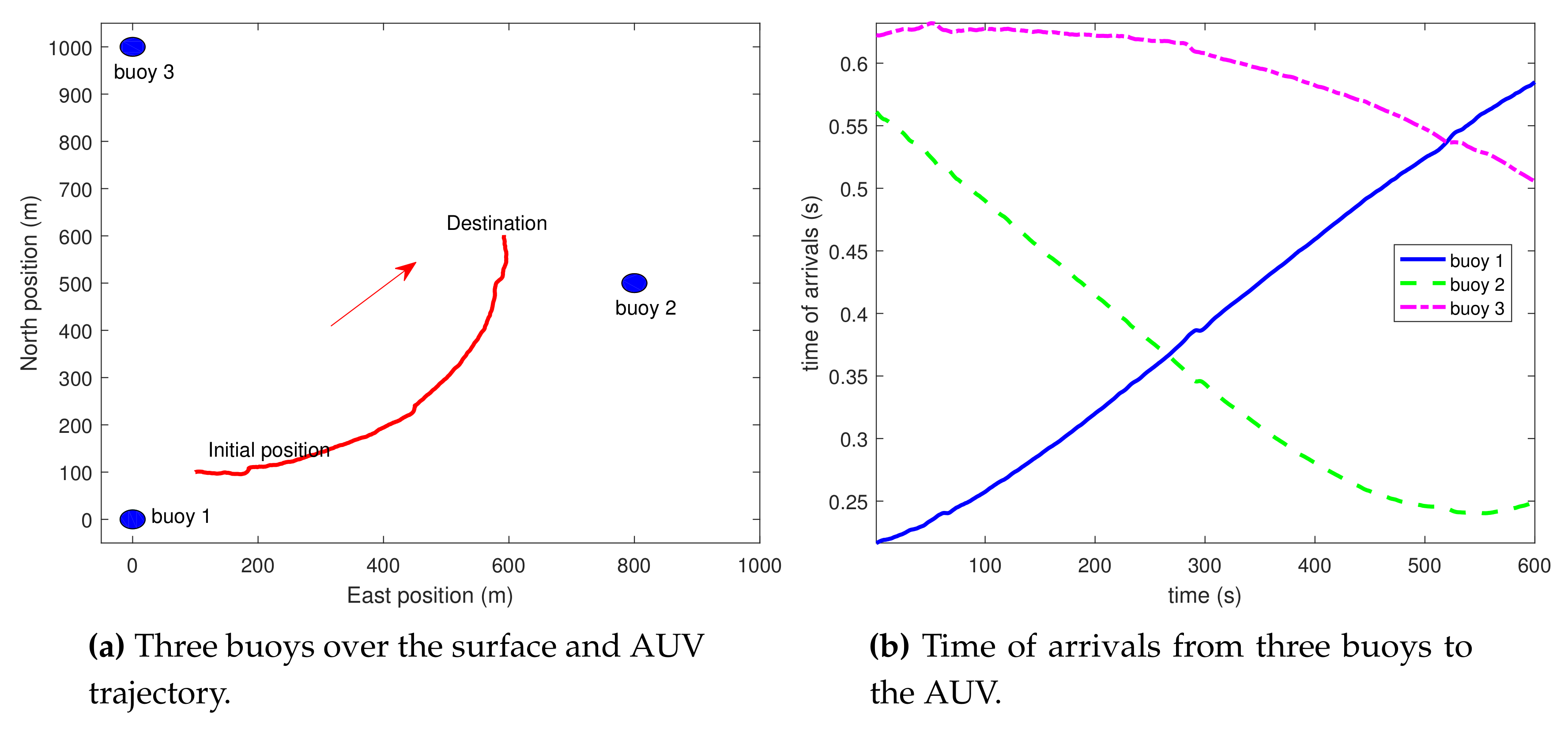
For the considered scenario, the three buoys are localized at the surface as shown in Figure 3a. The TOAs of the signals from the three buoys calculated by Equations (8)–(16) considering the isogradient SSP Equation (7) are plotted in Figure 3b. Since $T_{\mathrm{s}}^{\mathrm{l}}=1$ s, there are a total 600 TOAs being calculated for each buoy. As the AUV moves from the initial position to the destination, the distance between the AUV and buoy 1 is increasing while the distances between the AUV and buoys 2 and 3 are decreasing. Therefore, it is observed in Figure 3b that the TOA trajectory of buoy 1 ascends while the other two trajectories descend. Note that since the AUV approaches towards buoy 2 faster than buoy 3, the TOA trajectory of buoy 2 declines also more rapidly than that of buoy 3.

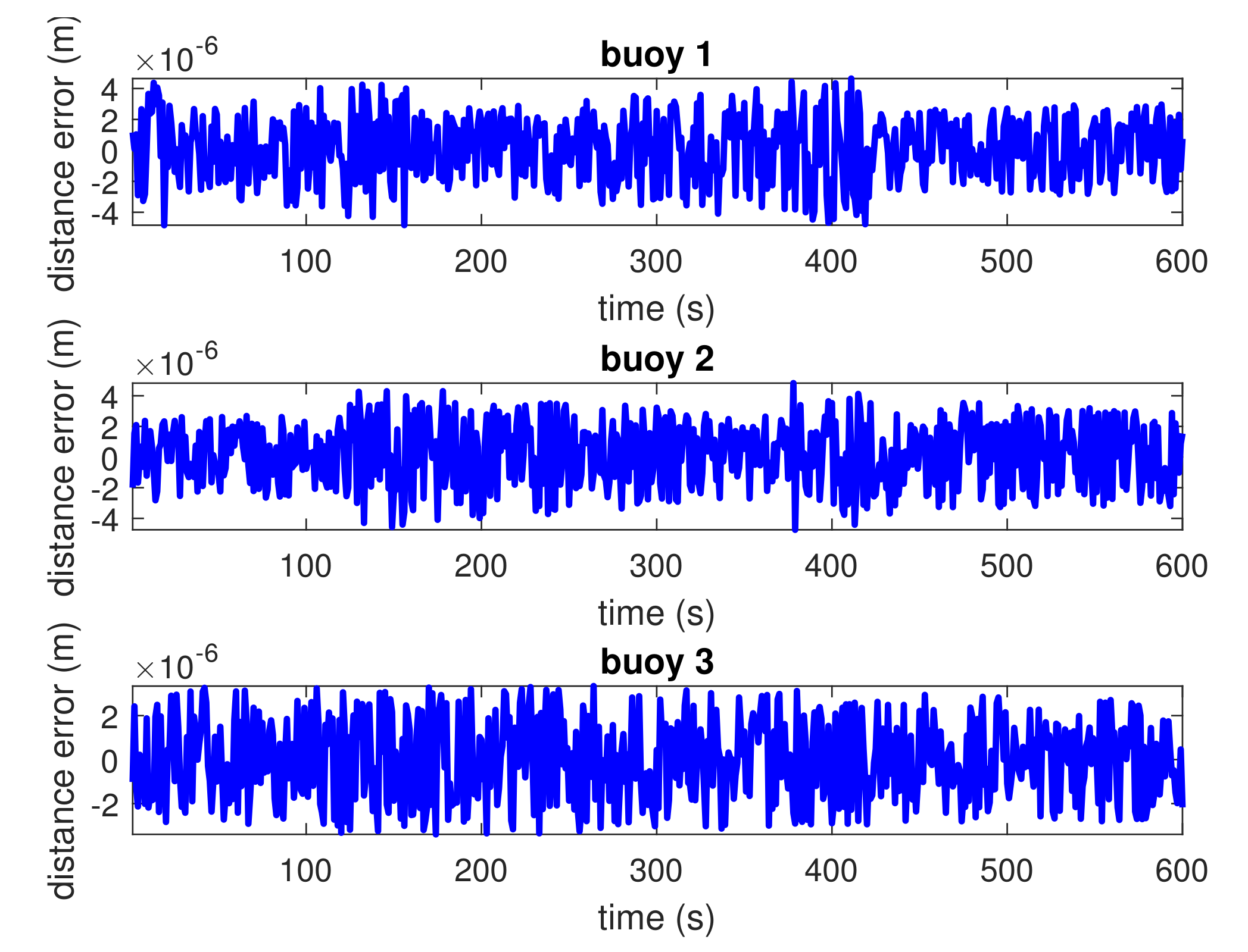
Figure 4 further shows the distance errors between the real horizontal distances $d_i\left(t\right)$ and the estimated horizontal distances ${\widehat{d}}_i\left(t\right)$ as calculated with a binary search algorithm [27]. Small distance errors are observed. The micrometer magnitude in Figure 4 is because the threshold specified in the binary search algorithm for the estimated horizontal distance is set to $1\times {10}^{-5}$. The binary search algorithm makes trade-offs in terms of speed and accuracy.

5.1.2. Tracking Control Results without Prediction Biased Errors

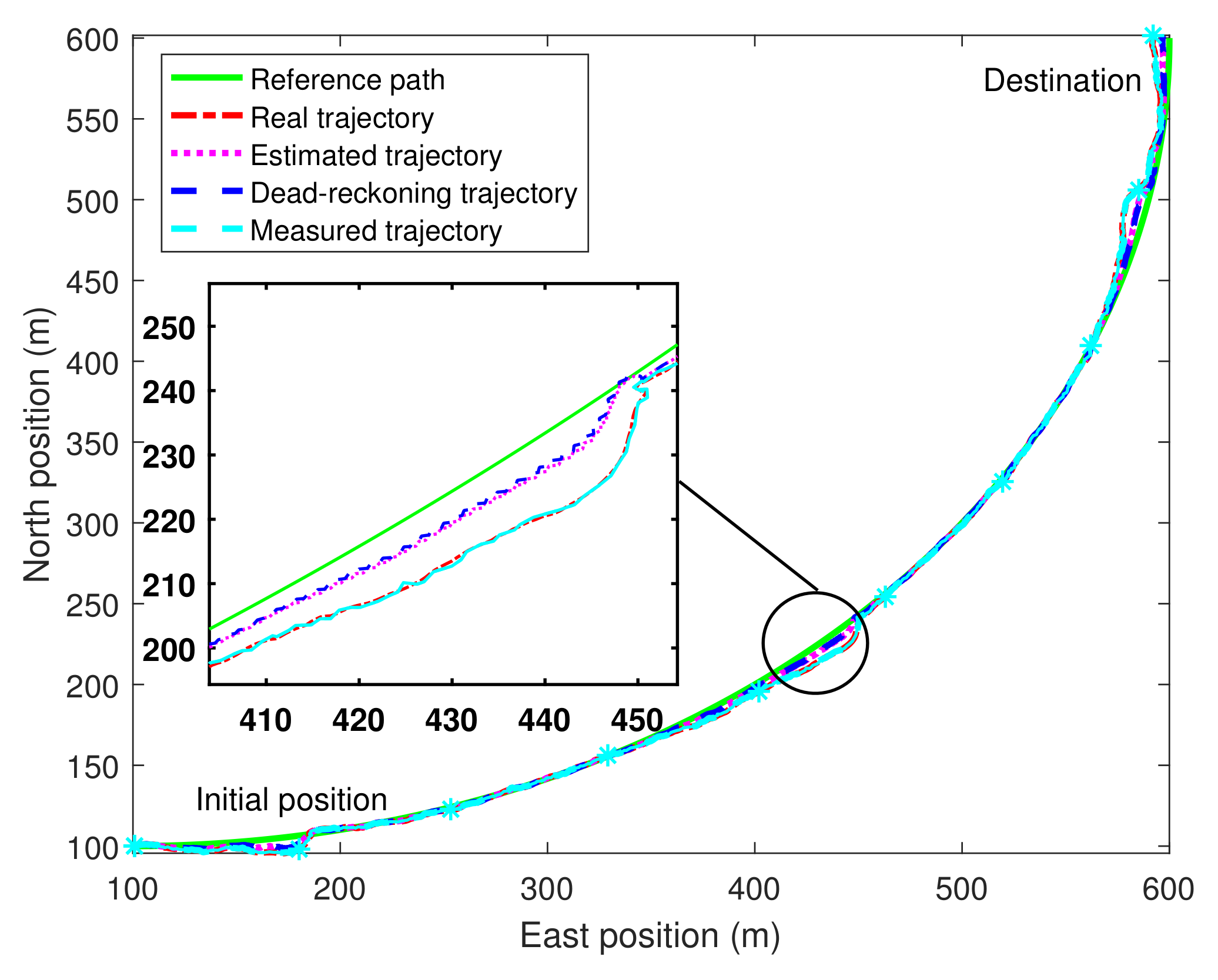
For the MPC controller design, system state feedback is necessary at each time step as in Equation (33). However, due to the uncertainties in system dynamics and measurements, only estimated system states from EKF or predicted system states from dead-reckoning with nominal system dynamics can be utilized. Figure 5 shows that the proposed algorithm can achieve the trajectory tracking goal and control the AUV moving from the initial position to the destination along the path. In Figure 5, five trajectories are plotted in total:

• The reference path is determined by connecting the initial position and the destination;
• The real AUV trajectory is $\mathit{x}\left(t\right)$ recorded from the simulations by evolving Equation (20) based on Equations (1) and (2) with known uncertain ocean currents.
• The estimated AUV trajectory $\widehat{\mathit{x}}\left(t\right)$ is the trajectory from the EKF, i.e., from Equation (26). This trajectory is obtained by correcting the dead-reckoning trajectory using the acoustic localization feedback information, i.e., the “measured” output, $\widehat{\mathit{y}}\left(t\right)$.
• The dead-reckoning trajectory $\overline{\mathit{x}}\left(t\right)$ is calculated from Equation (20) by ignoring the system uncertainties, i.e., Equation (28).
• The measured outputs $\mathit{y}\left(t\right)$ are obtained from Equation (18) by adding stochastic uncertainties at the computed results from the TOAs according to Equation (17) at each localization step.

Overall, the differences among these trajectories are small. Therefore, a zoom-in around position (300, 300) m is added. The root-mean-square-error for tracking the reference path is 5.59 m which is qualified in applications such as large-area ocean mapping. Note that the estimated trajectory and the measured trajectory are plotted with fewer position points than the dead-reckoning trajectory since the control cycle is faster than the acoustic localization cycle.

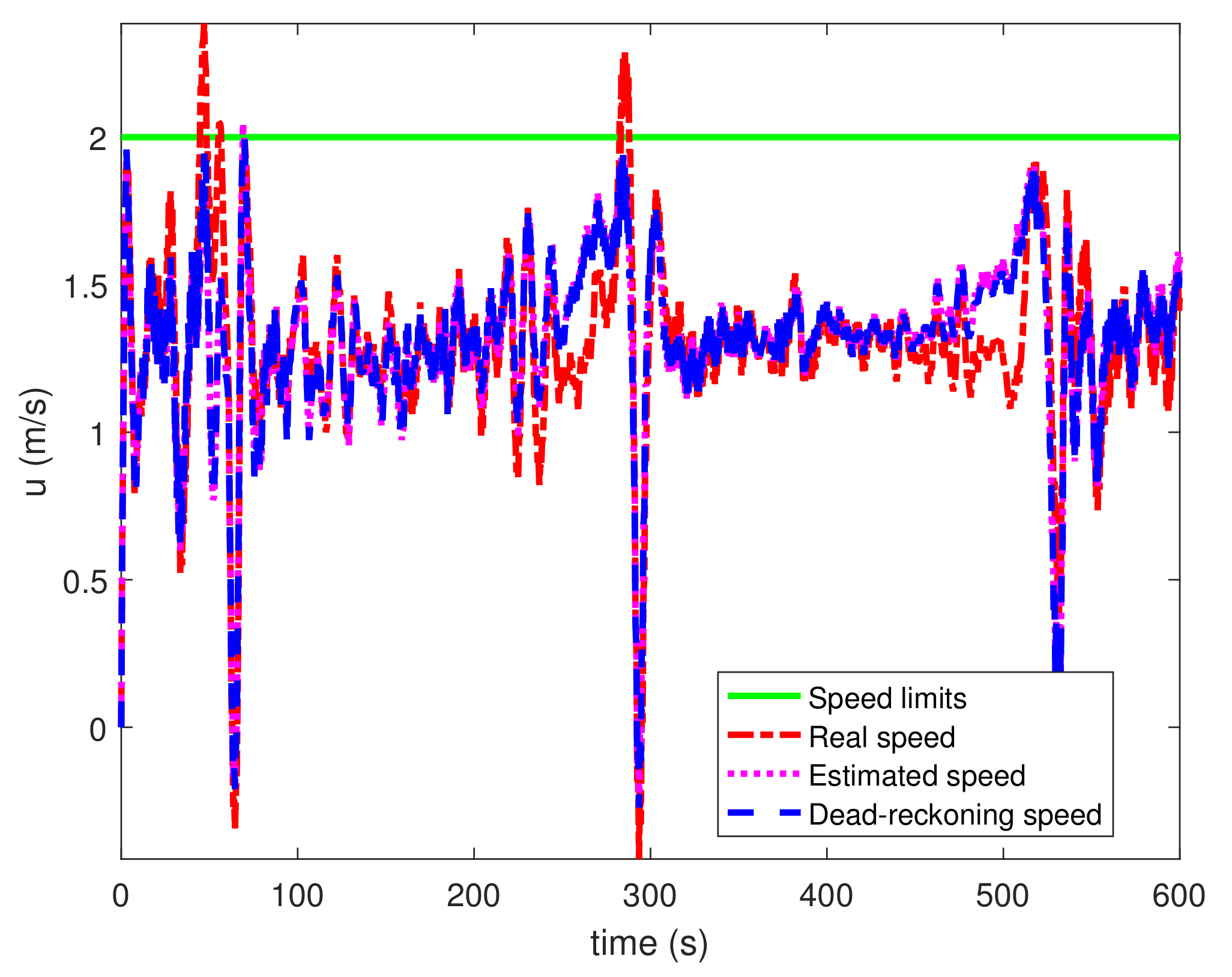
Figure 6 and Figure 7 show the speed and control input trajectories, respectively. The control inputs, i.e., the propeller thrust and the rudder angle, computed by solving the optimization problem Equation (32) subject to Equations (22), (33)–(36) all satisfy the system constraints. However, for the speed trajectory, the dead-reckoning speed trajectory satisfies the constraints well while small violations of the real and estimated trajectories with respect to the speed limits are observed. This is because both the optimization problem Equation (32) subject to Equations (22), (33)–(36) and the dead-reckoning trajectory use the nominal system dynamics without uncertainties. If all the constraints Equations (22), (33)–(36) are satisfied in the optimization problems, the dead-reckoning trajectory will also satisfy the constraints. However, compared to the dead-reckoning trajectory, the real trajectory further incorporates the uncertainties in ocean currents, and the estimated trajectory further incorporates the uncertainties in measurements. These uncertainties push the dead-reckoning trajectories that are already on the constraint boundary out of the feasible zone. Approaches such as buffer zone design in [31] can be applied to deal with this issue. Note that the differences between the estimated and dead-reckoning speed trajectories are small, and the root-mean-square-root value between these two trajectories is 0.03 m/s. This difference demonstrates the correction capability of the EKF as in Equation (26).

To relieve the potential computational burden of the MPC online optimization problems, successively linearized prediction models Equation (22) are used. Therefore, only linear programming online problems need to be solved. Figure 8 shows the solver times of the proposed tracking controller. Mostly throughout the simulation, the solver times are between 10 ms to 20 ms, and are smaller than the system control sampling time $T_{\mathrm{s}}^{\mathrm{c}}=0.5$ s, which indicates the potential of the proposed algorithm for real-time applications.

5.1.3. Tracking Control Results with Prediction Biased Errors

When there are biased errors in the predicted ocean current information, due to the inherent robustness of the MPC feedback control by using the updated states from acoustic localization, the AUV can still follow the reference path, as shown in Figure 9. However, compared to Figure 5 where there are no prediction biased errors, the AUV trajectory sees larger fluctuations. The root-mean-square-error for the reference tracking increases to 6.17 m compared to 5.59 m in the case of no biased errors. The larger tracking errors are partly due to the modeling errors, i.e., the error between the model used for the controller design and the model used for simulations. Furthermore, we also run a simulation where no ocean current information is used in the controller design, i.e., the predicted mean current speed, angle, and their covariances are all set to zero in the controller. In this case, infeasibilities occur and the simulation could not continue. Therefore, a proper consideration of the influence of ocean currents is necessary.

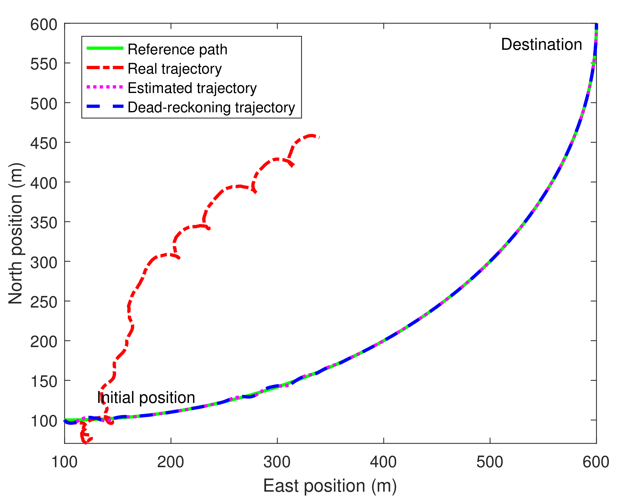
5.2. Tracking Control without Acoustic Localization

In order to demonstrate the role of acoustic localization for the AUV tracking control, we also run a set of simulations without acoustic localization. The system states used for MPC feedback are purely provided by the dead-reckoning module. This is the case when the AUV is not equipped with any positioning devices in an underwater environment. In this case, the AUV can never even reach the destination. Therefore, we set the simulation time the same as in the case with acoustic localization, and the tracking results are shown in Figure 10. It can be observed that the trajectory deviates far away from the reference path. The tracking task fails which means the tracking control algorithm with purely dead-reckoning is not acceptable in practical applications. Compared with Figure 5, Figure 10 further demonstrates the effectiveness of the proposed integrated acoustic localization and tracking control approach. Note that since no acoustic localization feedback is used, there is no measured trajectory and the estimated trajectory coincides with the dead-reckoning trajectory. Moreover, since now the controller is purely based on the dead-reckoning states which are subject to no disturbances, the dead-reckoning trajectory can follow the reference path well.

6. Conclusions and Future Work

For the two challenges that face the autonomy of AUVs, i.e., localization and ocean currents, this paper proposes a systematic approach. Firstly, the localization problem is solved with the aid of three surface buoys. By leveraging the different latencies of the three surface signals arriving at the AUV, the position of AUV can be calculated every localization cycle. The acoustically calculated position can then be utilized to correct the predicted and possible inaccurate position in dead-reckoning with EKF. Moreover, the uncertain ocean currents and full state reconstruction can also be incorporated in the framework of EKF. An MPC controller is designed to handle system constraints and control metrics based on the estimated full states from EKF. Simulation results demonstrate that the proposed integrated acoustic localization and tracking control approach outperforms the tracking control without acoustic localization. The potential of applying the proposed algorithm to AUVs is illustrated especially in addressing the challenges of underwater localization and ocean currents. Future research will consider extending the AUV dynamics to three dimensional space and the possibility of cooperative localization and control with multiple AUVs.

References

1. Wynn, R.B.; Huvenne, V.A. Autonomous underwater vehicles (AUVs): Their past, present and future contributions to the advancement of marine geoscience. Mar. Geol. 2014, 352, 451–468. [Google Scholar] [CrossRef] [Green Version]
2. Yuh, J.; Lakshmi, R. An intelligent control system for remotely operated vehicles. IEEE J. Ocean. Eng. 1993, 18, 55–62. [Google Scholar] [CrossRef]
3. Zhang, F.; Marani, G.; Smith, R.N.; Choi, H.T. Future trends in marine robotics. IEEE Robot. Autom. Mag. 2015, 22, 14–122. [Google Scholar] [CrossRef]
4. Tan, H.-P.; Diamant, R.; Seah, W.K.; Waldmeyer, M. A survey of techniques and challenges in underwater localization. Ocean Eng. 2011, 38, 1663–1676. [Google Scholar] [CrossRef] [Green Version]
5. Almeida, J.; Matias, B.; Ferreira, A.; Almeida, C.; Silva, E. Underwater localization system combining iUSBL with dynamic VAMOS in trials. Sensors 2020, 20, 4710. [Google Scholar] [CrossRef] [PubMed]
6. Torrieri, D.J. Statistical theory of passive location systems. IEEE Trans. Aerosp. Electron. Syst. 1984, 2, 183–198. [Google Scholar] [CrossRef] [Green Version]
7. Liu, Q.; Li, M. Discrete-Time Position Control for Autonomous Underwater Vehicle under Noisy Conditions. Appl. Sci. 2021, 11, 5790. [Google Scholar] [CrossRef]
8. Alcocer, A.; Oliveira, P.; Pascoal, A. Study and implementation of an EKF GIB-based underwater positioning system. Control Eng. Pract. 2007, 15, 689–701. [Google Scholar] [CrossRef]
9. Fan, S.; Li, B.; Xu, W.; Xu, Y. Impact of current disturbances on AUV docking: Model-based motion prediction and countering approaches. IEEE J. Ocean. Eng. 2017, 43, 888–904. [Google Scholar] [CrossRef]
10. Zhang, F. Cyber-maritime cycle: Autonomy of marine robots for ocean sensing. Found. Trends Robot. 2016, 5, 1–115. [Google Scholar] [CrossRef] [Green Version]
11. Pereira, A.A.; Binney, J.; Hollinger, G.A.; Sukhatme, G.S. Risk-aware path planning for autonomous underwater vehicles using predictive ocean models. J. Field Robot. 2013, 30, 741–762. [Google Scholar] [CrossRef]
12. Fu, M.; Wang, L. Finite-Time Path Following Control of an Underactuated Marine Surface Vessel with Input and Output Constraints. Appl. Sci. 2021, 10, 6447. [Google Scholar] [CrossRef]
13. Antonelli, G. On the use of adaptive/integral actions for six-degrees-of-freedom control of autonomous underwater vehicles. IEEE J. Ocean. Eng. 2007, 32, 300–312. [Google Scholar] [CrossRef]
14. Fossen, T.I. Handbook of Marine Craft Hydrodynamics and Motion Control; John Wiley and Sons Ltd.: West Sussex, UK, 2011. [Google Scholar]
15. Fossen, T.; Perez, T. Kalman filtering for positioning and heading control of ships and offshore rigs. IEEE Control Syst. 2009, 29, 32–46. [Google Scholar]
16. Sørensen, A.J.; Sagatun, S.I.; Fossen, T.I. Design of a dynamic positioning system using model-based control. Control Eng. Pract. 1996, 4, 359–368. [Google Scholar] [CrossRef]
17. Torsetnes, G.; Jouffroy, J.; Fossen, T.I. Nonlinear dynamic positioning of ships with gain-scheduled wave filtering. In Proceedings of the 43rd IEEE Conference on Decision and Control, Nassau, Bahamas, 14–17 December 2004; Volume 5, pp. 5340–5347. [Google Scholar]
18. Çetin, Ş.; Akkaya, A.V. Simulation and hybrid fuzzy-PID control for positioning of a hydraulic system. Nonlinear Dyn. 2010, 61, 465–476. [Google Scholar] [CrossRef]
19. Lapierre, L.; Jouvencel, B. Robust nonlinear path-following control of an AUV. IEEE J. Ocean. Eng. 2008, 33, 89–102. [Google Scholar] [CrossRef]
20. Tannuri, E.; Agostinho, A.; Morishita, H.; Moratelli, L., Jr. Dynamic positioning systems: An experimental analysis of sliding mode control. Control. Pract. 2010, 18, 1121–1132. [Google Scholar] [CrossRef]
21. Mayne, D.Q. Model predictive control: Recent developments and future promise. Automatica 2014, 50, 2967–2986. [Google Scholar] [CrossRef]
22. Uchihori, H.; Cavanini, L.; Tasaki, M. Linear Parameter-Varying Model Predictive Control of AUV for Docking Scenarios. Appl. Sci. 2021, 11, 4368. [Google Scholar] [CrossRef]
23. Shen, C. Motion Control of Autonomous Underwater Vehicles Using Advanced Model Predictive Control Strategy. Ph.D. Thesis, University of Victoria, Victoria, BC, Canada, 2018. [Google Scholar]
24. Saback, R.M.; Conceicao, A.G.S.; Santos, T.L.M.; Albiez, J.; Reis, M. Nonlinear model predictive control applied to an autonomous underwater vehicle. IEEE J. Ocean. Eng. 2019, 45, 799–812. [Google Scholar] [CrossRef]
25. Prestero, T.T.J. Verification of a Six-Degree of Freedom Simulation Model for the REMUS Autonomous Underwater Vehicle. Ph.D. Thesis, Massachusetts Institute of Technology, Cambridge, MA, USA, 2001. [Google Scholar]
26. Yayla, G.; Senne, B.; Gerben, P.; Muhammad, A. Accuracy Benchmark of Galileo and EGNOS for Inland Waterways. In Proceedings of the International Ship Control Systems Symposium, Delft, The Netherlands, 6–8 October 2020. [Google Scholar]
27. Ramezani, H.; Jamali-Rad, H.; Leus, G. Target localization and tracking for an isogradient sound speed profile. IEEE Trans. Signal Process. 2013, 61, 1434–1446. [Google Scholar] [CrossRef]
28. Paull, L.; Saeedi, S.; Seto, M. AUV Navigation and Localization: A Review. IEEE J. Ocean. Eng. 2014, 39, 131–149. [Google Scholar] [CrossRef]
29. MATLAB. R2016b. Available online: https://www.mathworks.com/products/matlab.html (accessed on 29 August 2021).
30. Zheng, H.; Negenborn, R.R.; Lodewijks, G. Trajectory tracking of autonomous vessels using model predictive control. In Proceedings of the 19th IFAC World Congress, Cape Town, South Africa, 24–29 August 2014; pp. 8812–8818. [Google Scholar]
31. Zheng, H.; Negenborn, R.R.; Lodewijks, G. Predictive path following with arrival time awareness for waterborne AGVs. Transp. Res. Part C Emerg. Technol. 2016, 70, 214–237. [Google Scholar] [CrossRef]
32. ILOG. IBM ILOG CPLEX Optimizer. Available online: http://www-01.ibm.com/software/integration/optimization/cplex-optimizer/ (accessed on 7 January 2016).
Figure 1. AUV motions in the inertial coordinate system { n } and the body-fixed coordinate system { b } with ocean currents in the horizontal plane.
Applsci 11 08038 g001
Figure 2. AUV localization with three surface buoys.
Applsci 11 08038 g002
Figure 3. Time of arrivals considering the sound speed profile.
Applsci 11 08038 g003
Figure 4. Errors between the real horizontal distance and the estimated horizontal distance.
Applsci 11 08038 g004
Figure 5. AUV tracking control trajectories: real- x ( t ) , estimated- x ^ ( t ) , dead-reckoning- x ¯ ( t ) , and measured- y ( t ) .
Applsci 11 08038 g005
Figure 6. Speed trajectories and constraints.
Applsci 11 08038 g006
Figure 7. Input trajectories and constraints.
Applsci 11 08038 g007
Figure 8. Solver times of the MPC online optimization problems.
Applsci 11 08038 g008
Figure 9. AUV tracking control trajectories with prediction biased errors: real- x ( t ) , estimated- x ^ ( t ) , dead-reckoning- x ¯ ( t ) , and measured- y ( t ) .
Applsci 11 08038 g009
Figure 10. AUV tracking control trajectories without acoustic localization: real- x ( t ) , estimated- x ^ ( t ) , and dead-reckoning- x ¯ ( t ) .
Applsci 11 08038 g010
Publisher’s Note: MDPI stays neutral with regard to jurisdictional claims in published maps and institutional affiliations.