Article

Ellipsoidal Path Planning for Unmanned Aerial Vehicles

by
Carlos Villaseñor
1,
Alberto A. Gallegos
2,
Gehova Lopez-Gonzalez
2,
Javier Gomez-Avila
1,
Jesus Hernandez-Barragan
1 and
Nancy Arana-Daniel
1,*
1
Department of Computer Science, University of Guadalajara, 1421 Marcelino García Barragán, Guadalajara 44430, Mexico
2
Department of Artificial Intelligence, Neural10 S de RL de CV, Av. Aviación 5051, Zapopan 45019, Mexico
*
Author to whom correspondence should be addressed.
Appl. Sci. 2021, 11(17), 7997; https://doi.org/10.3390/app11177997
Submission received: 4 June 2021 / Revised: 23 August 2021 / Accepted: 26 August 2021 / Published: 29 August 2021
(This article belongs to the Special Issue Applied Machine Learning Ⅱ)

Abstract

:
The research in path planning for unmanned aerial vehicles (UAV) is an active topic nowadays. The path planning strategy highly depends on the map abstraction available. In a previous work, we presented an ellipsoidal mapping algorithm (EMA) that was designed using covariance ellipsoids and clustering algorithms. The EMA computes compact in-memory maps, but still with enough information to accurately represent the environment and to be useful for robot navigation algorithms. In this work, we develop a novel path planning algorithm based on a bio-inspired algorithm for navigation in the ellipsoidal map. Our approach overcomes the problem that there is no closed formula to calculate the distance between two ellipsoidal surfaces, so it was approximated using a trained neural network. The presented path planning algorithm takes advantage of ellipsoid entities to represent obstacles and compute paths for small UAVs regardless of the concavity of these obstacles, in a very geometrically explicit way. Furthermore, our method can also be used to plan routes in dynamical environments without adding any computational cost.

1. Introduction

Autonomous Unmanned Aerial Vehicles (UAVs) play an important role in both military and civilian applications. In contrast with manned aircrafts, UAVs are able to perform complex and dangerous tasks with high maneuverability and low cost [1,2]. An important problem to solve in order to achieve a certain level of autonomy is path planning. In the past, the best path was selected as the shortest distance to a goal; now, the best path is associated with the traveled distance and energy consumption [3]. If more parameters, besides distance, are considered, the path planning problem can been stated as an optimization problem, and population based algorithms have been used in many cases to solve it successfully [4,5,6,7,8].
In [9], we described a novel algorithm for path planning, which uses conformal geometric algebra to generate maps using spheres. By using spheres, we gain in terms of the number of parameters needed for representing the maps and these maps are rich in information. For example, we need the same number of parameters for representing a sphere as for a plane, but the plane also needs an extra number of parameters for bounding the plain. Moreover, the spheres are easy to operate in conformal geometric algebra.
The algorithm employs the characteristics of the spheres described in this algebra to navigate through the maps by combining them with Teaching-Learning Based Optimization (TLBO). In this paper, we compared different evolutionary optimization algorithms where TLBO had the best result.
On the other hand, we also explored approaching the robotic mapping problem by using ellipsoidal representations [10]. These ellipsoidal geometric entities are coded in the geometric algebra G 6 , 3 . The resulting map is compact and rich in information as we showed in [10].
The problem of robotic mapping consists of constructing a spatial representation of the environment, which is helpful for the robot [11]. There are classic mapping abstractions, such as grid occupancy [12], where cubes represent the objects. This abstraction is memory efficient but discretizes the environment; furthermore, it is useful for office-like environments but is not adequately suited for outdoor environments.
We can also find variable size grid occupancy [13], where we can change the resolution of the grid. With particular modification, we can model dynamic maps with this abstraction [14].
There are other map abstractions such as multiplanar maps [15], landmarks, and points of obstacles [16]. A mapping algorithm called OctoMap was proposed in [17,18]. OctoMap has variable resolution grid occupancy representation with a probabilistic construction. We include in Table 1 a qualitative comparison between ellipsoidal maps and Octomap.
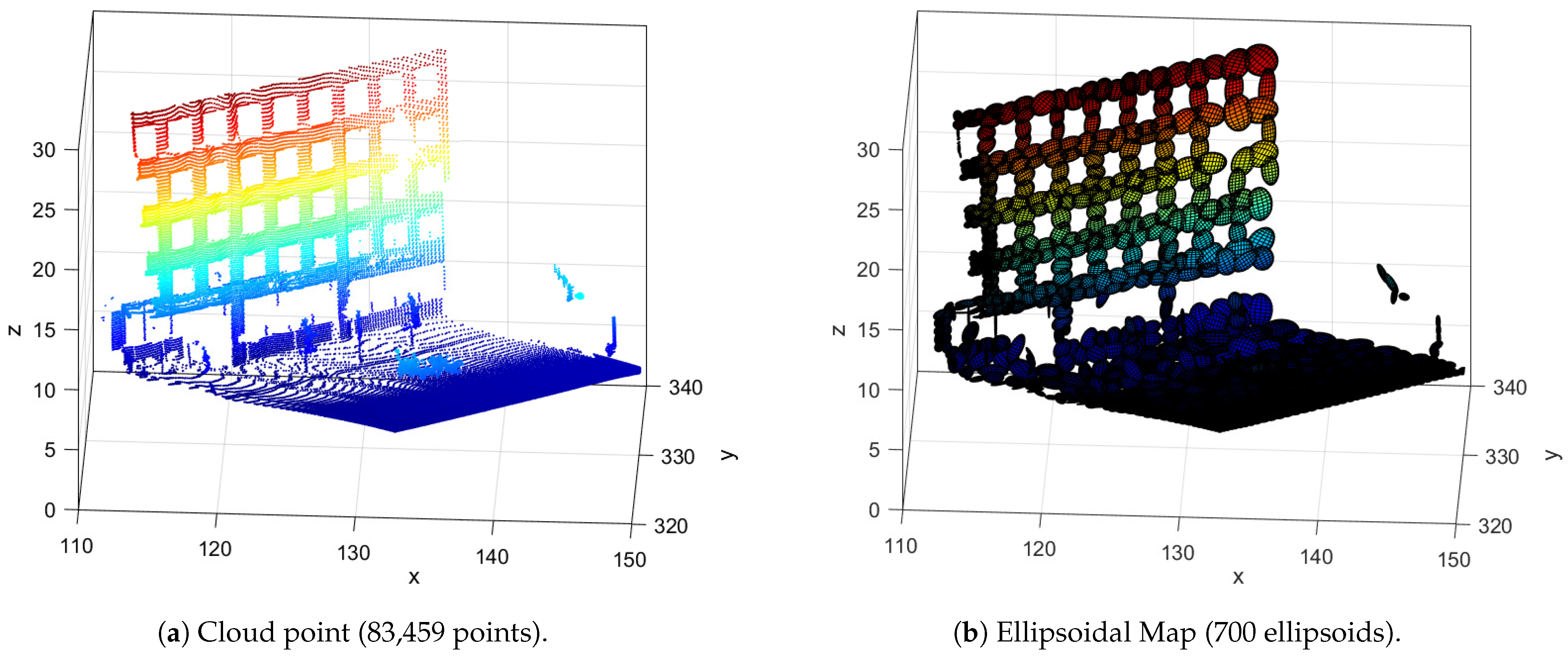
In Figure 1, we present an example of a cloud point (left) [19] and its ellipsoidal map (right).
In this work, we present a novel algorithm for path planning in 3D environments for small UAVs. This algorithm works on ellipsoidal mapping provided by the algorithm in [10]. There is no closed form for calculating the distance between two ellipsoidal surfaces and using an iterative algorithm will be computational expensive.
We propose to solve this problem by training a dense neural network for approximating the distance between two ellipsoids. We propose a new fitness function to find the path with the TLBO algorithm.
The TLBO algorithm was chosen because it obtained the best performance in a similar problem presented in [9]. We refer the reader to [9] for a performance comparison on metaheuristics for similar path-planning.
The paper is organized as follows: in Section 2, we introduce our solution to efficiently calculate the distance between ellipsoids and we show the training and generalization results. In Section 3, we offer a brief review of the TLBO algorithm and we develop the fitness function for path planning in ellipsoidal maps. Then, the simulation and results of the proposed algorithm are presented in Section 4. Finally, in Section 5, we offer a conclusion and future directions based on this work.

2. Approximating the Distance Function with Neural Networks

Our goal was to develop a path planning algorithm to work with the ellipsoidal maps to take advantage of these maps being compact-in-memory yet rich-in-information. The hypothesis to achieve the above goal was to design an algorithm that could compute a path using the distance between the envelope ellipsoids of the obstacles, and the ellipsoid that models the UAV. The computed path maintains the vehicle safe free space between itself and the occupied places.
To know how much free space exists between ellipsoids, we needed to solve the non-trivial key problem of finding a method to compute the distance between them due to the fact that there is not a closed way to do it. We propose a machine learning method to solve the above computation using neural networks to overcome the problem that represents the great computational costs of using iterative algorithms to calculate distances in maps, where the number of ellipsoids is large.
To solve this problem efficiently, we use a dense neural network to estimate the distance between two ellipsoids. One ellipsoid will represent a small UAV and the other will represent an obstacle.
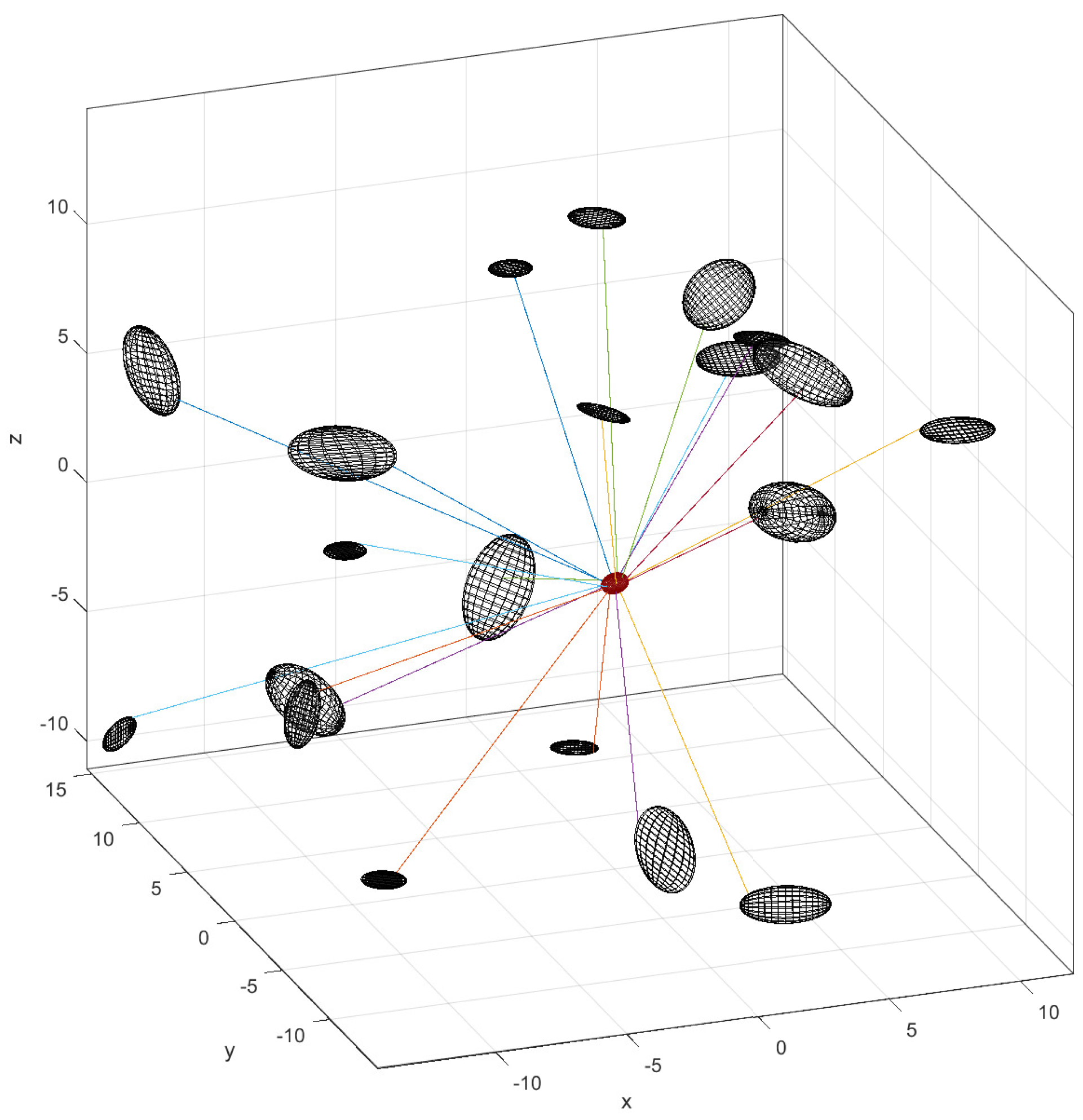
We can train a neural network for the regression problem. To generate a dataset for training, we randomly generate a pose for the UAV (yaw, pitch and roll). We fix the semi-axes of the ellipsoid representing the UAV with ( 0.5 , 0.5 , 0.3 ) in meters. Furthermore, we generate a random ellipsoid around the UAV. We calculate a cloud mesh for every ellipsoid and estimate the distance between the UAV by using a brute force approach. In Figure 2, we present an example of generated samples and their estimated distance.
One problem with this approach is to find a correct normalization of the data. If the input data of a neural network is not well normalized it could lead to slow or biased learning. In the following, we describe a novel normalization method that achieves good results on the neural network performance.
Firstly, the small UAV is represented by an ellipsoid with fixed semi-axes. These semi-axes are not considered in the learning problem, because the neural network can learn them as well. We will fix the UAV position at the center of the 3D space. Then, the position and the semi-axes are not input data for the neural network. The UAV is represented only with the angles ( y a w , p i t c h , r o l l ) [ 0 , 2 π ] 3 .
In the second instance, the 3D points on the map representing the obstacles are mapped using ellipsoids. As we presented in [10], we applied a clustering technique to the cloud point. Each cluster is a set of 3D points [ x i , y i , z i ] T i = 1 n , with center of mass [ μ x , μ y , μ z ] T .
We can also calculate the pair-wise covariance between two variables; for example, for x and y coordinates, the covariance is calculated with (1):
σ x y = σ y x = i = 1 n ( x i μ x ) ( y i μ y ) n .
With the pair-wise covariances, we construct the covariance matrix is defined with (2). The parameters ( c 1 , , c 9 ) carry the information of an ellipsoid that covers all non-outlier data points.
= σ x x σ x y σ x z σ x y σ y y σ y z σ x z σ y z σ z z = c 1 c 2 c 3 c 4 c 5 c 6 c 7 c 8 c 9 .
The obstacle ellipsoids will be represented with the normalized covariance matrix. This parametrization is chosen because it is the output of the multi-ellipsoidal mapping algorithm presented in [10]. Other parametrizations lead to a high computational cost; for instance, one could use the angles of rotation and the semi-axes, but this will require the spectral decomposition of the covariance matrix.
In Figure 3, we present a 2D scheme of the maximum and minimum distances between two ellipses. The desired distance will be between the minimum and the maximum distances and it will depend on the orientation of the ellipses.
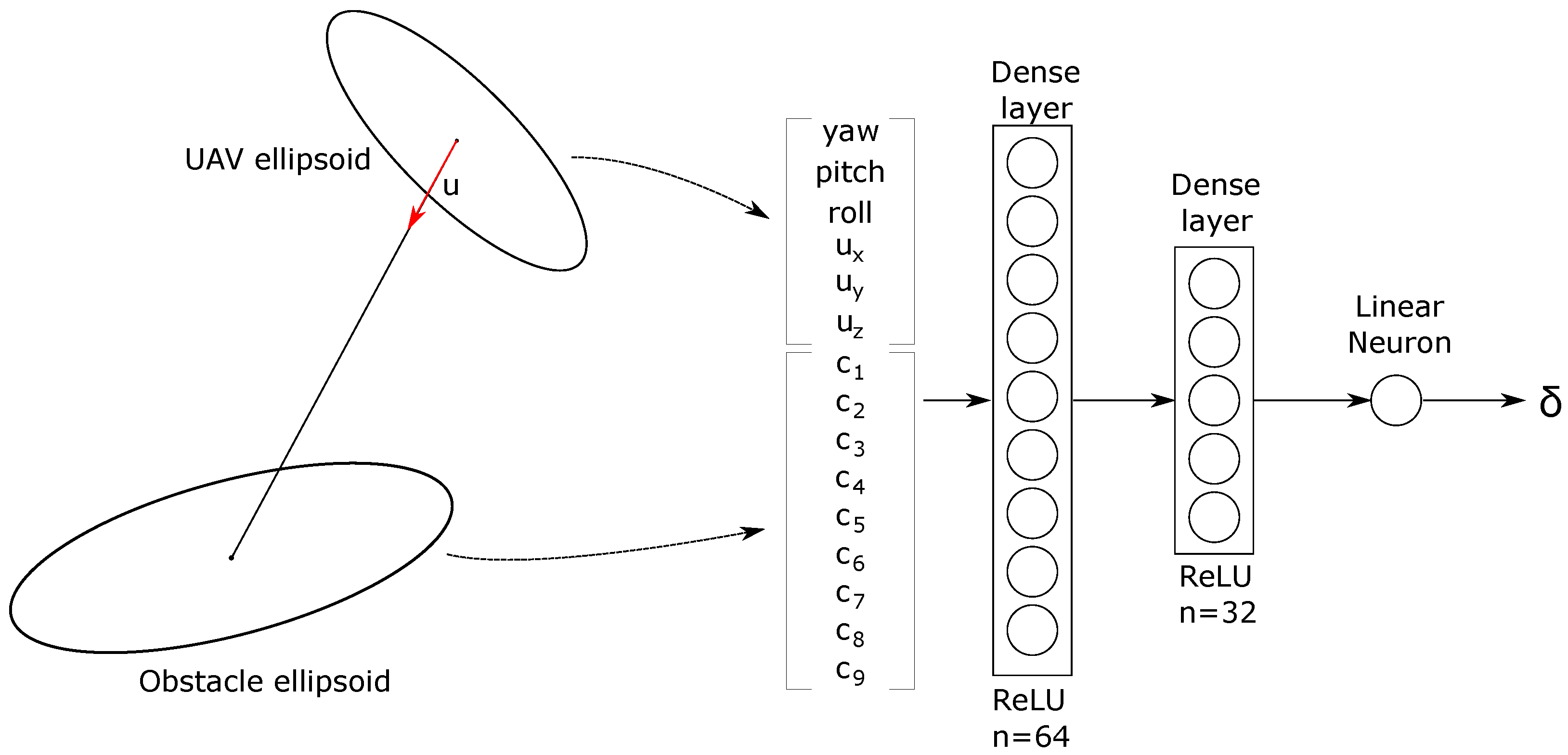
The positions of the UAV and obstacles are difficult to normalize. If we normalize using common techniques like max-min or the standard normalization the neural network could output strange values for ellipsoid outside this normalization. To avoid this situation, we will code the relative position with a normalized vector from the UAV center to the obstacle center ( u x , u y , u z ) .
Instead of doing regression with the real distance between the ellipsoids, we just estimate a correction variable δ if we subtract this value from the centers distance of the ellipsoids, we can calculate the distance between ellipsoids, as we show in (3):
d i s t ( E 1 , E 2 ) = | | Center 1 Center 2 | | 2 δ .
The δ correction factor depends only on the relative position of the obstacle ellipsoid and the UAV ellipsoid and their orientations. We can approximate this correction factor with a neural network. In Figure 4, we present the normalized input vector and the neural network architecture.
We generate 185,000 random examples that took one day to calculate. We distribute these samples the following way: 149,850 samples for training, 16,650 for validating and hyper-parameter tuning, and 18,500 for testing. We trained this neural network for 50 epochs. In Figure 5, we show the training and validation evolution on the mean squared error (MSE). We got 0.0016 final MSE for training and 0.0017 final MSE for validation.
In Table 2, we present the training results. In particular, we present the R 2 -score where the best possible value is one, we also show the mean absolute error (MAE) and the median absolute error (MedianAE), in order to give a good sense of the capabilities of the neural network.
The neural network achieves a high performance in predicting the correction factor and by using (3), we can accurately calculate the distance between the UAV and the obstacle ellipsoids. The Network was programmed on Keras/Tensorflow, then the network natively can run on a graphical process unit (GPU) for high performance. After testing, we can calculate the distance between a UAV ellipsoid and 200 obstacles in a mean time of 0.1208 s (We use a RTX 2060 GPU). With this result, we can assure that the application of path planning over ellipsoidal maps is computationally affordable.
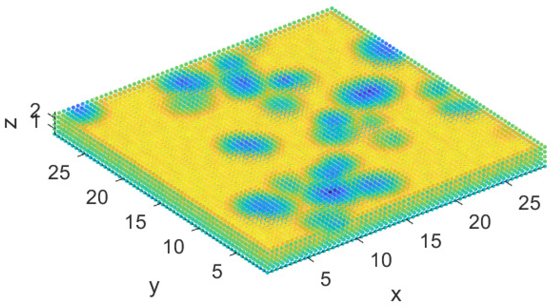
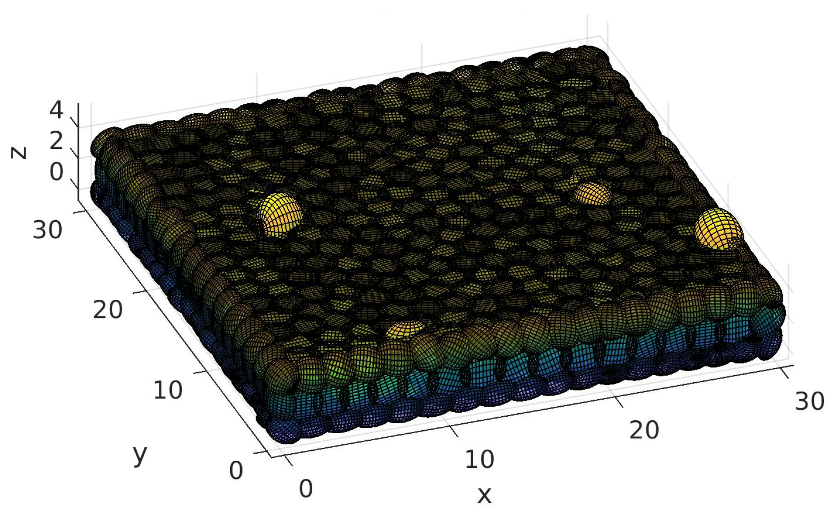
Finally, we run an experiment on a virtual environment by placing the UAV in a grid position and calculating the minimum distance to the closest object. In Figure 6, we show the result of the experiment. The warmer colors represent greater distances. Notice that the neural network can calculate an accurate map that is compact in memory and rich in information.
In the next section, we develop the path planning algorithm based on this neural network by using a bio-inspired algorithm with a greedy approach.

3. Teaching-Learning Based Optimization

TLBO is an optimization algorithm based on the teaching of knowledge from a teacher to his or her students on a classroom [20]. This population based algorithm has two main phases, in which it generates new knowledge: the teacher and the learner phase.
The teacher phase is inspired by the transmission of knowledge from a teacher to the students, and centers efforts to increase the average score of the class. The learner phase is inspired by the knowledge shared among students; the students with more information will be beneficial as the other learners learn new information from them. The teacher is the best solution so far in the current iteration.

3.1. Teacher Phase

A good teacher will try to increase the knowledge of the students/learners based on his or her own knowledge over time/iterations. But no matter how good a teacher is, because of many factors this can only be done to some extent in a classroom composed of n students. It can be said that the mean of the new knowledge of the class will be moved in some extent towards the teacher’s knowledge, but it will also depend on the capabilities of the class [21].
The following equation shows the intent of the teacher X T to influence, to some degree, each individual X i (composed of the drones ( x , y , z , y a w , p i t c h , r o l l ) values) with the help of the mean of knowledge of the whole class x ¯ :
X i = X i + r ( X T T f x ¯ ) ,
where T f { 1 , 2 } is a random value of only two possible values, named the teaching factor; and r [ 0 , 1 ] is a random number. If  f ( X i ) provides a better solution than f ( X i ) (where f is a fitness function), X i replaces X i as a solution.

3.2. Learner Phase

The learner phase depends on the interchange of knowledge between students. A learner with new information will have an influence on the overall knowledge of the class [22].
This phase consists of adjusting each learner X i based on another learner X k , where i and k [ 1 , n ] : i k [9].
There are two alternatives that could happen for learners X; when the f ( X i ) is better than f ( X k ) which generates the following learner:
X i = X i + r ( X i X k )
or vice versa, when f ( X k ) is better than f ( X i ) ,
X i = X i + r ( X k X i ) ,
X i replaces X i as a solution if it represents a better solution. As can be seen, this phase also includes the teacher solution from the previous phase, but in a less important role.

3.3. Fitness Function

We designed a fitness function that is composed of four terms:
f ( X i ) = d t + c + h ( d t + 1 ) + s ( d t + 1 ) ,
where d t is the Euclidean distance between a learner X i and the target point θ (composed of only by x, y and z values); by itself this term helps to attract the population towards the target. c is the obstacle collision indicator:
c = if any o j 0 , 0 otherwise
where o j is the distance between the leaner X i and the obstacle j, which is obtained using the neural network described in Section 2. The collision indicator’s function is to heavily penalize collisions, since it is of utmost importance to guarantee the UAV’s safety.
h represents a heat factor that indicates the proximity of X i to a set of obstacles o d o j : 0 < o d r 1 , where r 1 is a user defined range of proximity:
h = ( l o g 2 ( 0.001 o d ) + l o g 2 ( r 1 ) ) .
To give the drone the capability to avoid large convex obstacles inside a room (usually obstacles that go from floor to ceiling), a stuck factor s is added. To obtain s it is necessary to create a set of stuck zones s z ; when the euclidean distance of the ( x , y , z ) values of teachers τ t 1 and τ t (where τ is the last teacher obtained from a TLBO run and t is the current run) is less than a user defined threshold α , a zone is added to s z . If the condition is met the ( x , y , z ) values from τ t are queued to s z . The stuck factor is obtained as follows:
s = ( l o g 2 ( 0.001 s k ) + l o g 2 ( r 2 ) ) ,
where s k is the set of Euclidean distances from a learner X i to any point in s z , where 0 < s k r 2 , and  r 2 represents a user defined range of proximity. The pseudocode for path planning is presented in Algorithm 1.
Algorithm 1 Path Planning Algorithm.
1:
procedure Optimize
2:
     a c t u a l _ p o s starting position
3:
     X i create learner population
4:
     X i initialize to zero
5:
     X T obtain teacher from population as a separate value
6:
     n g e n s number of generations
7:
     s t o p stopping value
8:
     t q u e u e teachers queue
9:
     S z set stuck zones list to empty
10:
     X T f i t n e s s f i t n e s s ( X i , S z )
11:
     α 0.1                                                                                                       ▹ User defined threshold
12:
    while  X T f i t n e s s > s t o p  do
13:
         for  g e n 1 to n g e n s  do
14:
               for every X i  do
15:
                      X i t e a c h e r _ p h a s e ( X i )                                         ▹ This step corresponds to (4)
16:
                      X i b o u n d _ i n c r e m e n t s ( X i , a c t u a l _ p o s )
17:
                X i f i t n e s s f i t n e s s ( X i , S z )                                                                       ▹ Evaluates (7)
18:
                X i s e l e c t _ b e s t ( X i , X i )              ▹ Selects the best candidate between X i and X i
19:
               for every X i  do
20:
                      X i l e a r n e r _ p h a s e ( X i )                            ▹ This step corresponds to (5) and (6)
21:
                      X i b o u n d _ i n c r e m e n t s ( X i , a c t u a l _ p o s )               ▹ Described in Section 4
22:
               X i f i t n e s s f i t n e s s ( X i , S z )
23:
              ( X i , X i f i t n e s s ) s e l e c t _ b e s t _ l e a r n e r s ( ( X i , X i f i t n e s s ) , ( X i , X i f i t n e s s ) )
24:
               ( X T , X T f i t n e s s ) u p d a t e _ t e a c h e r ( X i , X i f i t n e s s )
25:
           t q u e u e a p p e n d ( X T , t q u e u e )                                                             ▹ Add X T to queue
26:
           d i s t = n o r m ( X T [ 0 : 3 ] a c t u a l _ p o s [ 0 : 3 ] )                                     ▹ Euclidean norm
27:
           a c t u a l _ p o s X T
28:
           X i i n i t i a l i z e ( )                                                          ▹ Initialize and obtain fitness values
29:
           X i s e t _ t o _ z e r o ( )
30:
           m i m a x _ i n d e x ( X i f i t n e s s )
31:
          if  d i s t < α  then
32:
               S z a p p e n d ( X T )
33:
          else
34:
                 X m i X T
    return  t q u e u e

4. Simulation and Results

To define the whole path, TLBO was run several times, and each time (except the first one) the learners were initialized randomly within the proximity of τ t 1 ; for the first iteration the ( x , y , z , y a w , p i t c h , r o l l ) base values where defined arbitrarily. Each TLBO run consisted of 20 iterations and a population of five individuals; r 1 and r 2 were assigned values of 0.35 and 1.5 , respectably. As a stopping condition, the Euclidean distance from τ t and the target θ was used (a distance value less than 0.1). At the end of a run, τ t is added to the path. As Figure 7 shows.
The values that could be achieved by a learner were bounded, so that the drone could not make abrupt changes that could make it behave unstably from one state to another or fly at very pronounced angles. In each iteration, the values of the learners were bounded by τ t 1 ± ( 0.5 , 0.5 , 0.5 , 0.15 , 0.15 , 0.25 ) . The drone’s ( y a w , p i t c h , r o l l ) values were also bounded globally to ± [ π , 0.7 , 0.7 ] radians, respectively. The bounds and other values were empirically selected. We included the pitch and roll angles in the search space because some control schemes for UAV such as Backstepping or Inverse Optimal Control need these references [23,24,25]. However, our proposal can work even when ignoring pitch and roll angles.
Compared to [9], our approach involving the path planning algorithm offers several advantages. Firstly, our approach was designed to work indoors and outdoors alike. Ref. [9] shows several limitations avoiding large convex obstacles inside a room since it does not take them into consideration and this prevents the algorithm to be trapped in certain local minimums. Tthe influence of the obstacles in our approach also only takes into account the nearest obstacles in the range and adds smaller penalty values that do not heavily obfuscate the influence of the distance to a target in the fitness function.
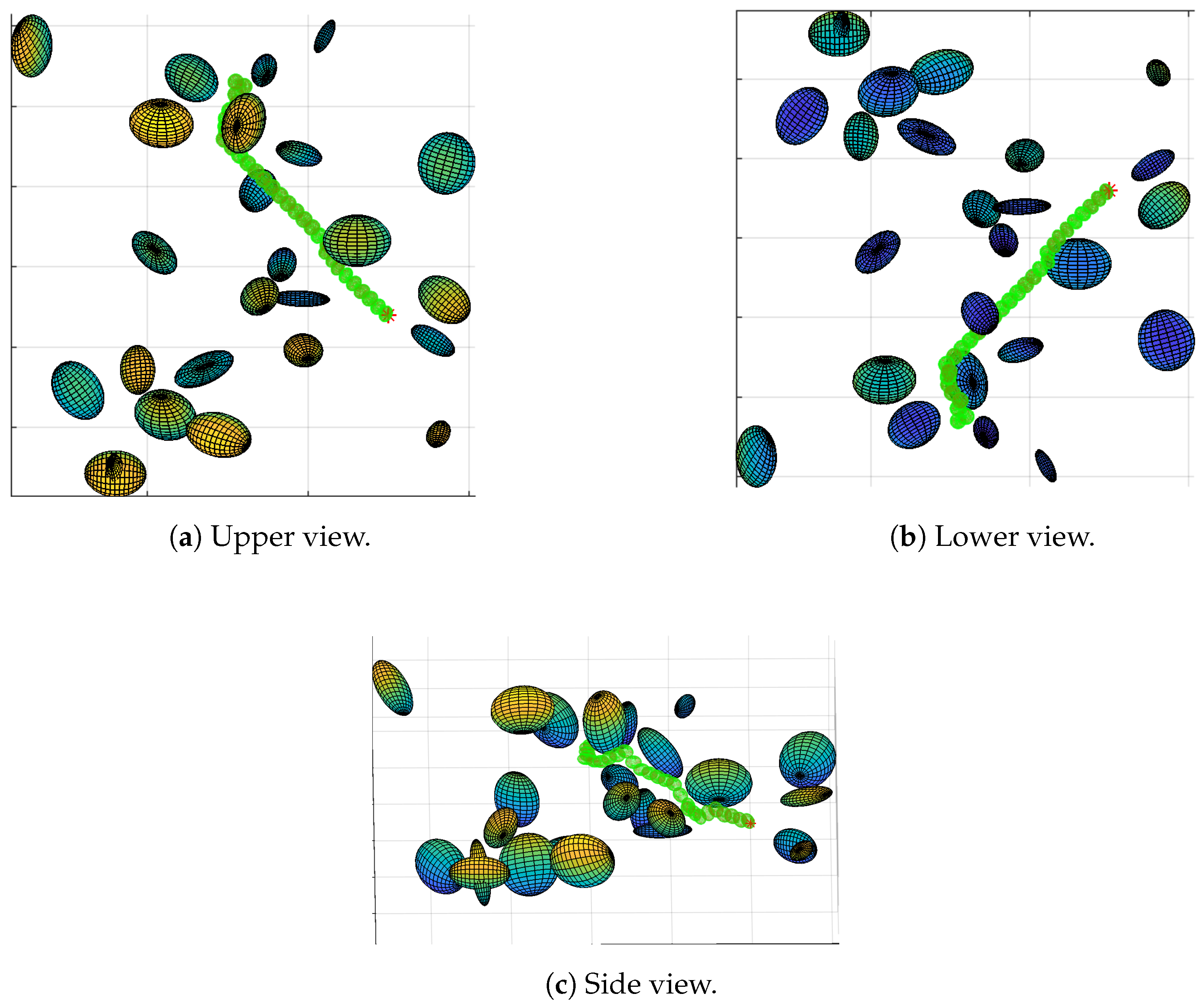
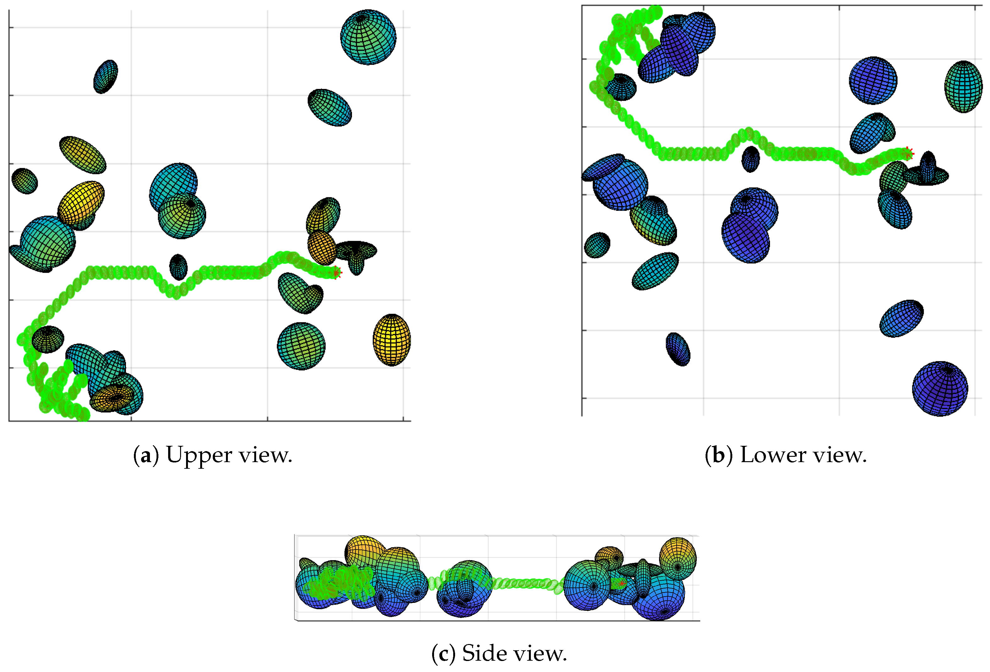
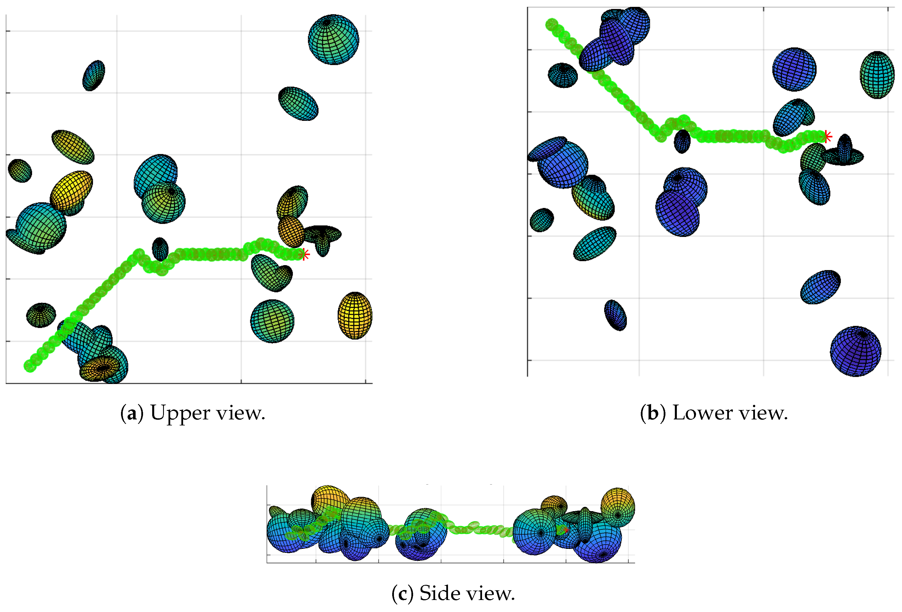
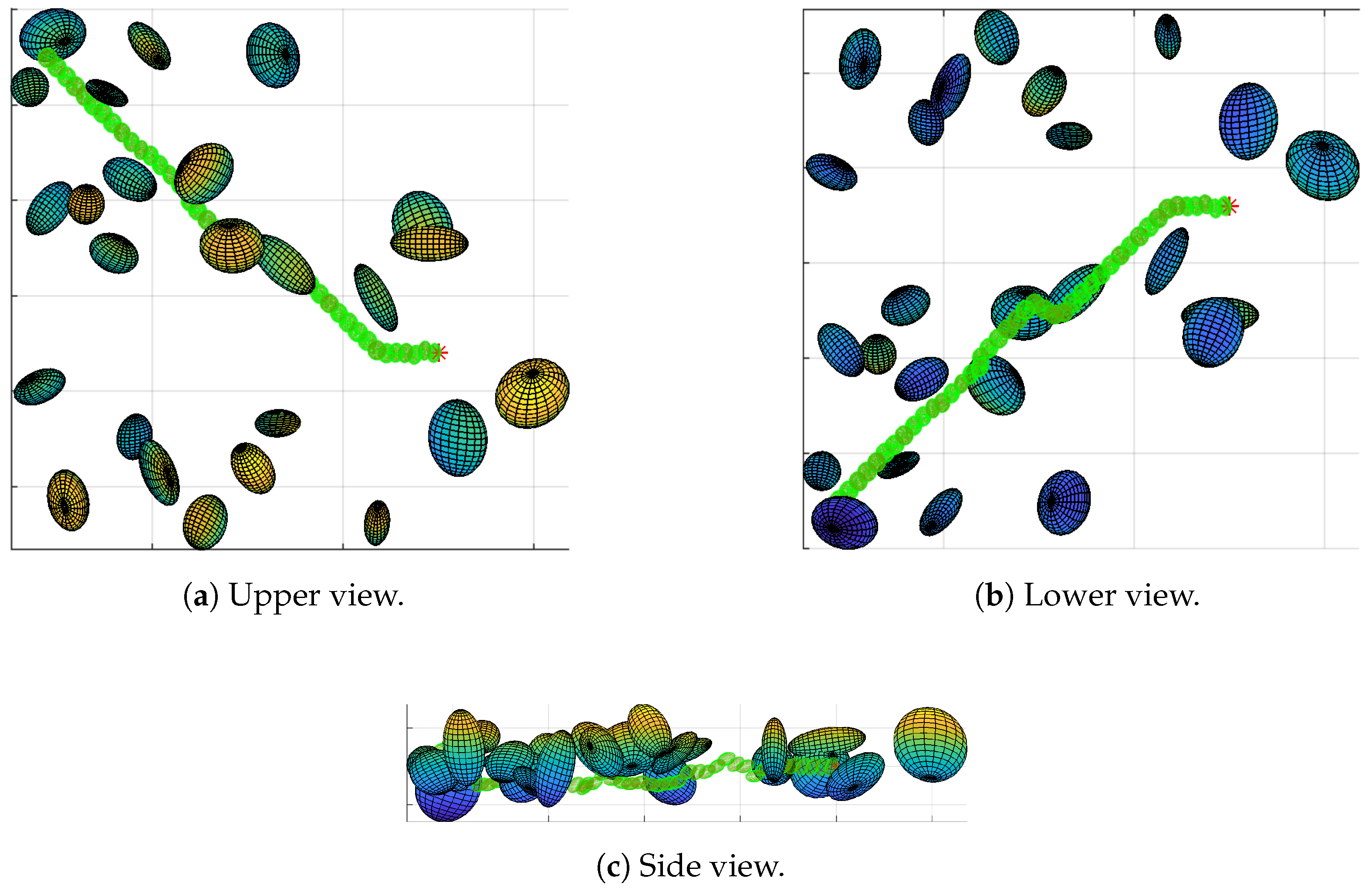
Figure 8, Figure 9, Figure 10, Figure 11 and 
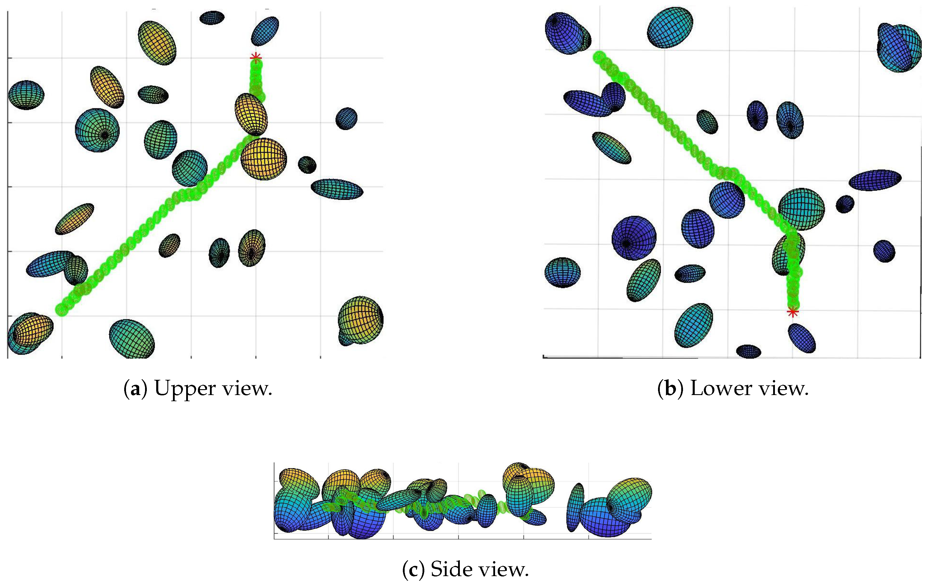
Figure 12 show several maps where paths were generated for a drone to follow. All the maps were contained in a room composed of ellipsoids. The room was not plotted for display purposes.
The figures display the path followed by the drone (green ellipsoids) to its target (red asterisk), avoiding on the way several obstacles (multicolor ellipsoids). As can be seen, the drone can easily follow the paths obtained by the algorithm. Maps, like those shown in Figure 8 and Figure 9, show little difficulty finding a path; even in the presence of convex obstacles at the start, the drone is safely pushed away until it finds a way to circumnavigate the obstacles. Comparing Figure 9 and Figure 10 it can be seen that, without the room, the path simply passes above and beside the obstacles.

Comparison with State of the Art Algorithms

In order to validate the proposed method, we compared it with other evolutionary techniques and a well-known path planning algorithm. Firstly, we describe the Rapidly-exploring Random Tree Star (RRT*) [26].
The RRT* algorithm, presented in Algorithm 2, finds a free path from the initial point z i n i t to the final point z g o a l . We created a tree T with an initial node z i n i t . Next, we grew the tree up for N attempts.
Algorithm 2 Rapidly-exploring Random Tree Star (RRT*)
1:
T InitializeTree()
2:
T InsertNode(, z i n i t , T)
3:
for i = 1 to N do
4:
     z r a n d SampleSpace()
5:
     z n e a r e s t Nearest(T, z r a n d )
6:
     ( z n e w , U n e w ) Steer( z n e a r e s t , z r a n d )
7:
    if ObstacleFree( z n e w ) then
8:
         z n e a r Near(T, z n e w )
9:
         z m i n ChooseParent( z n e a r , z n e a r e s t , z n e w )
10:
         T InsertNode( z m i n , z n e w , T)
11:
         T Rewire(T, z n e a r , z m i n , z n e w )
returnT
To find the next node in the tree, we randomly sampled a point on the map z r a n d that is not with an obstacle. We found the nearest node of the tree and renamed it z n e a r e s t . After steering from z n e a r e s t to z r a n d , this function has heuristics about the robot’s kinematics. Then we renamed z r a n d as z n e w and found a path U n e w .
The ObstacleFree function search for collision with obstacles on the line from z n e a r e s t to z n e w ; if there were no collisions, we proceeded to add the z n e w point. We collected the points close to z n e w within a certain radius. Then we chose the parent node that carried the least cost and renamed z m i n . Finally, we added the link between z m i n and z n e w and rewired the tree to find the minimum cost.
To apply the RRT* algorithm on an ellipsoidal map we developed a collision detection function. We used the Cholesky factorization of the covariance matrices that represent the obstacles. We show this in (11). In the case of the evolutionary algorithms, we can expect longer run-times because of the neural network prediction.
= L L T .
Using the triangular matrix L, we can calculate if a point x is inside an ellipsoid on the map by using the inequality (12), where μ is the center of the ellipsoid.
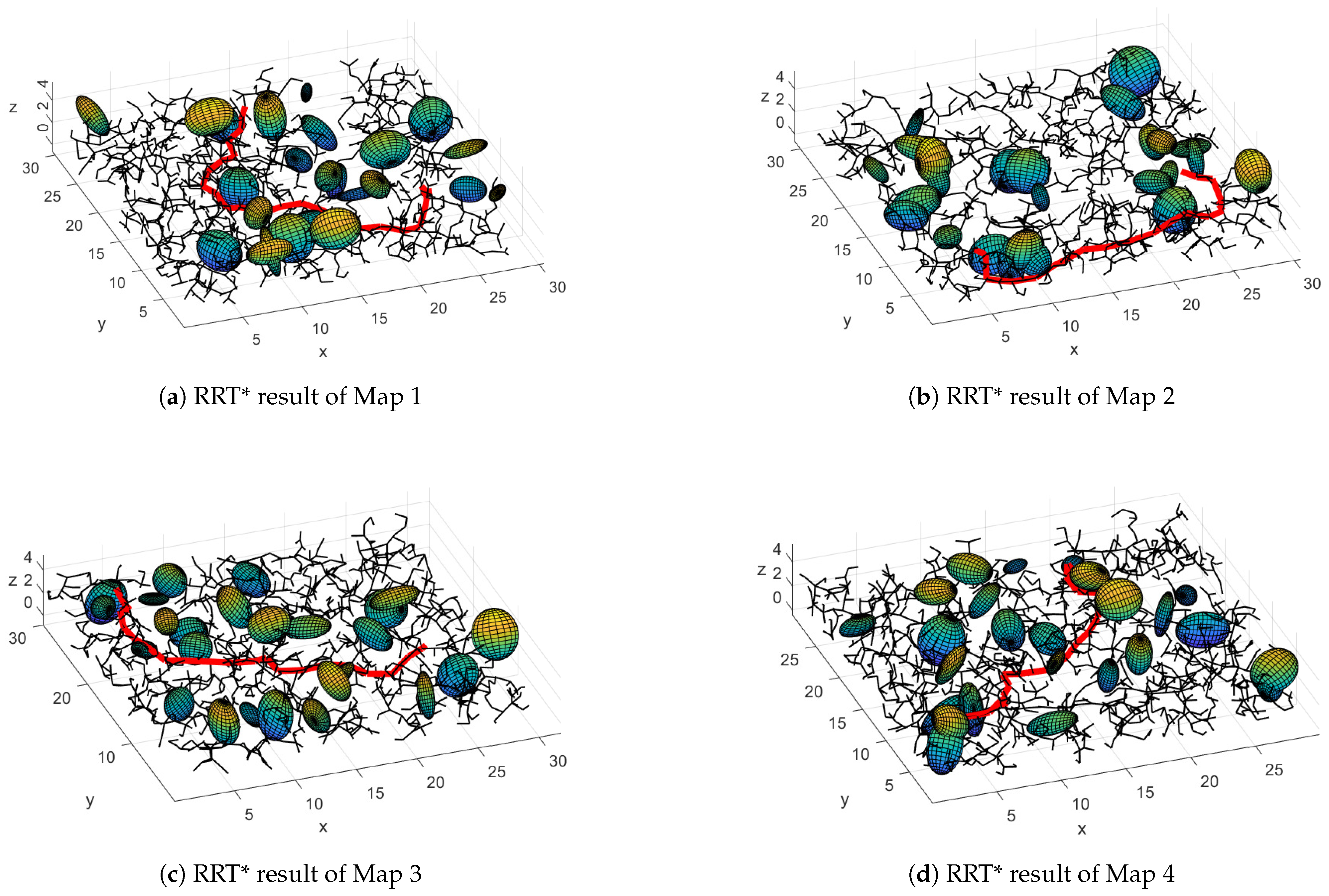
| | L T ( x μ ) | | 2 1 .
In Figure 13, we show the resulting path of the RRT* algorithm in the same four maps. Notice that the found paths avoid the obstacles but do not consider the ellipsoid that represents the UAV. We used a maximum of 5000 iterations, but for the mean convergence on the four maps it was 1348 iterations.
Furthermore, we also present experiments with other state-of-the-art evolutionary optimization algorithms. We ran the same tests for the the Differential Evolution (DE) [27] algorithm, the Particle Swarm Optimization (PSO) [28] algorithm, and the Firefly (FF) [29] algorithm.
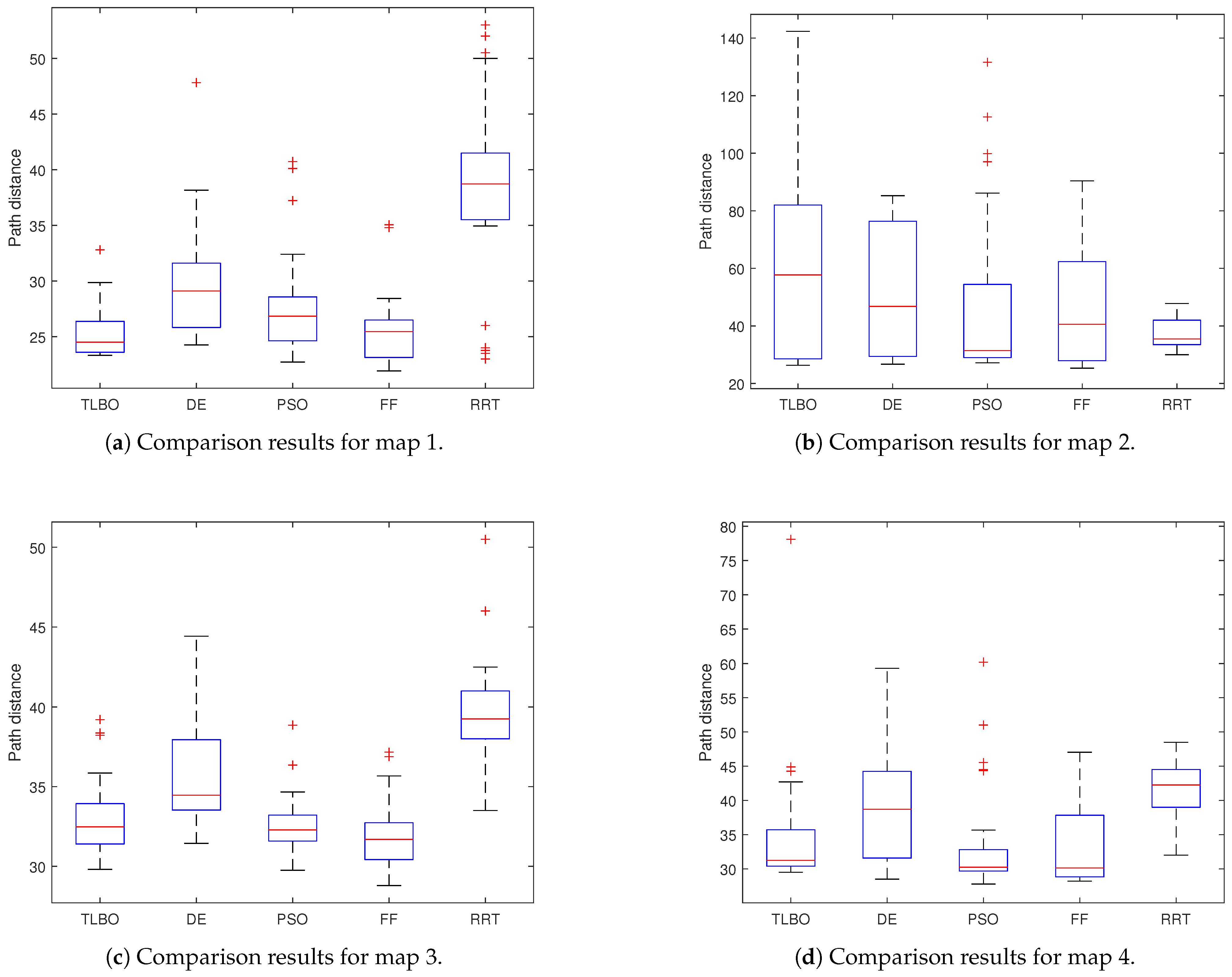
All the evolutionary algorithms used the same fitness function presented in (7). All the proposed methods are non-deterministic. To ensure the validity of the results, we ran each algorithm experiment 30 times on the same computer. The start and endpoints were the same for all the experiments. In Table 3, we present the comparison of the different methods. Notice that the evolutionary schemes have the best mean performance for maps 1, 3, and 4. In Figure 14, we show the box-and-whisker plots for each map and each method.
In Table 4, we include the number of steps in each evolutionary algorithm and the number of nodes in the RRT* algorithm.
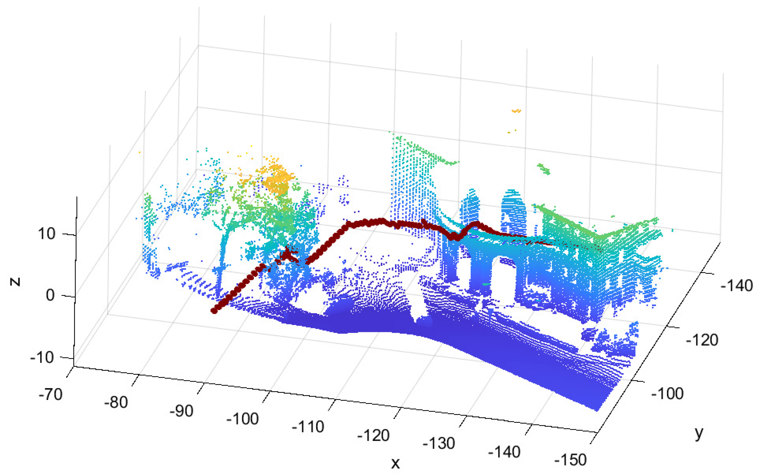
We proved the novel algorithm in a real environment. We used the map from [19], and we created the ellipsoidal map. In Figure 15, we offer the resulting path planning. Notice that this path planning has a good performance even in non-structural environments. In Table 5, we show how the Cholesky factorization allows lower complexity in the RRT* algorithm.

5. Conclusions and Future Work

In this work we presented a geometrically explicit and simple algorithm that takes advantage of the ellipsoidal representation of maps generated to plan collision-free and smooth paths regardless of the concavity of the obstacles or whether the environment is indoor or outdoor.
Our method solves the non-trivial problem of computing the distance between two ellipsoids by using a neural network. To train the neural network, it was necessary to produce a training dataset and design a novel normalization method for these data. So, we obtain an accurate approximation for the distance, which allows the computation of the free-space and occupied-space of an environment, as is shown in Table 2 and Figure 6.
In order to obtain paths and to keep the computational costs of our approach low, a bio-inspired algorithm named TLBO was used. We have chosen TLBO because it has had the best performance in previous comparisons with other techniques [9]. The fitness function was designed taking into account four desired features for the path obtained: to keep a safe distance between obstacles’ ellipsoids and the UAV ellipsoid; to avoid collisions; to reduce the total amount of the UAV’s proximity range throughout the whole path; and to give the drone the capability to avoid large convex obstacles (walls inside a room, dense and tall vegetation).
It is important to mention that, based on our design of the fitness function, the computed paths are not optimal. Because it was used as a greedy approach, it cannot get the optimal path but is more versatile and can manage dynamical maps without extra computational costs.
We compare the proposed approach with other evolutionary algorithms, DE, PSO, and FF. We also compare with RRT*, and we constructed the collision detection function for the ellipsoidal map. In most cases, evolutionary techniques with the presented fitness function obtained a better performance than RRT*, but clearly RRT* has a better performance on time. Furthermore, the evolutionary methods also calculate the UAV orientation and not just the ( x , y , z ) position.

Future Work

The proposed algorithm uses a greedy strategy to find a nearby optimal position. Therefore, the algorithm is locally optimal. To compare different path planning algorithms, a cost function must be developed, which has non dependency on the map abstraction.
We are working on substituting the greedy politic used to compute the path as well as the bio-inspired algorithm by a reinforcement learning algorithm so the system can learn policies of navigation instead of computing paths.
Furthermore, we are designing an intelligent low-level control algorithm that considers the dynamical model of the UAV to follow the planned path.

Author Contributions

Conceptualization, C.V. and J.H.-B.; methodology, C.V. and A.A.G.; software, A.A.G.; validation, G.L.-G. and J.G.-A.; writing—original draft preparation, J.G.-A.; writing—review and editing, G.L.-G.; visualization, J.H.-B.; supervision, N.A.-D.; project administration, C.V. and N.A.-D. All authors have read and agreed to the published version of the manuscript.

Funding

This research was funded by CONACYT México grants numbers CB256769, CB258068, and PN-4107.

Institutional Review Board Statement

Not applicable.

Informed Consent Statement

Not applicable.

Data Availability Statement

No applicable.

Conflicts of Interest

The authors declare no conflict of interest. The founders had no role in the design of the study; in the collection, analyses, or interpretation of data; in the writing of the manuscript, or in the decision to publish the results.

References

  1. Zhou, X.; Gao, F.; Fang, X.; Lan, Z. Improved Bat Algorithm for UAV Path Planning in Three-Dimensional Space. IEEE Access 2021, 9, 20100–20116. [Google Scholar] [CrossRef]
  2. Bolourian, N.; Hammad, A. LiDAR-equipped UAV path planning considering potential locations of defects for bridge inspection. Autom. Constr. 2020, 117, 103250. [Google Scholar] [CrossRef]
  3. Roberge, V.; Tarbouchi, M.; Labonté, G. Comparison of parallel genetic algorithm and particle swarm optimization for real-time UAV path planning. IEEE Trans. Ind. Inform. 2012, 9, 132–141. [Google Scholar] [CrossRef]
  4. Fan, M.; Akhter, Y. A Time-Varying Adaptive Inertia Weight based Modified PSO Algorithm for UAV Path Planning. In Proceedings of the 2021 2nd International Conference on Robotics, Electrical and Signal Processing Techniques (ICREST), Dhaka, Bangladesh, 5–7 January 2021; pp. 573–576. [Google Scholar]
  5. Shao, S.; Peng, Y.; He, C.; Du, Y. Efficient path planning for UAV formation via comprehensively improved particle swarm optimization. ISA Trans. 2020, 97, 415–430. [Google Scholar] [CrossRef]
  6. Ever, Y.K. Using simplified swarm optimization on path planning for intelligent mobile robot. Procedia Comput. Sci. 2017, 120, 83–90. [Google Scholar] [CrossRef]
  7. Arana-Daniel, N.; Gallegos, A.A.; López-Franco, C.; Alanis, A.Y. Smooth global and local path planning for mobile robot using particle swarm optimization, radial basis functions, splines and Bézier curves. In Proceedings of the 2014 IEEE Congress on Evolutionary Computation (CEC), Beijing, China, 6–11 July 2014; pp. 175–182. [Google Scholar]
  8. Arana-Daniel, N.; Gallegos, A.A.; López-Franco, C.; Alanis, A.Y. Smooth path planning for mobile robot using particle swarm optimization and radial basis functions. In Proceedings of the International Conference on Genetic and Evolutionary Methods (GEM), Las Vegas, NV, USA, 16–19 July 2012; p. 1. [Google Scholar]
  9. Hernandez-Barragan, J. Mobile Robot Path Planning based on Conformal Geometric Algebra and Teaching-Learning Based Optimization. IFAC-PapersOnLine 2018, 51, 338–343. [Google Scholar] [CrossRef]
  10. Villaseñor, C.; Arana-Daniel, N.; Alanis, A.Y.; Lopez-Franco, C.; Gomez-Avila, J. Multiellipsoidal Mapping Algorithm. Appl. Sci. 2018, 8, 1239. [Google Scholar] [CrossRef] [Green Version]
  11. Thrun, S. Robotic Mapping: A Survey. In Exploring Artificial Intelligence in the New Millennium; Morgan Kaufmann Publishers Inc.: San Francisco, CA, USA, 2003; pp. 1–35. [Google Scholar]
  12. Collins, T.; Collins, J.; Ryan, D. Occupancy grid mapping: An empirical evaluation. In Proceedings of the 2007 Mediterranean Conference on Control & Automation, Athens, Greece, 27–29 June 2007; pp. 1–6. [Google Scholar]
  13. O’Meadhra, C.; Tabib, W.; Michael, N. Variable resolution occupancy mapping using gaussian mixture models. IEEE Robot. Autom. Lett. 2018, 4, 2015–2022. [Google Scholar] [CrossRef]
  14. Meyer-Delius, D.; Beinhofer, M.; Burgard, W. Occupancy grid models for robot mapping in changing environments. In Proceedings of the Twenty-Sixth AAAI Conference on Artificial Intelligence, Toronto, ON, Canada, 22–26 July 2012. [Google Scholar]
  15. Thrun, S.; Burgard, W.; Chakrabarti, D.; Emery, R.; Liu, Y.; Martin, C. A real-time algorithm for acquiring multi-planar volumetric models with mobile robots. In Robotics Research; Springer: Berlin/Heidelberg, Germany, 2003; pp. 21–35. [Google Scholar]
  16. Sola, J. Simulataneous Localization and Mapping with the Extended Kalman Filter. Avery Quick Guide with MATLAB Code. 2013. Available online: https://www.iri.upc.edu/people/jsola/JoanSola/objectes/curs_SLAM/SLAM2D/SLAM%20course.pdf (accessed on 25 August 2021).
  17. Hornung, A.; Wurm, K.M.; Bennewitz, M.; Stachniss, C.; Burgard, W. OctoMap: An efficient probabilistic 3D mapping framework based on octrees. Auton. Robot. 2013, 34, 189. [Google Scholar] [CrossRef] [Green Version]
  18. Wurm, K.M.; Hornung, A.; Bennewitz, M.; Stachniss, C.; Burgard, W. OctoMap: A probabilistic, flexible, and compact 3D map representation for robotic systems. In Proceedings of the ICRA 2010 Workshop on Best Practice in 3D Perception and Modeling for Mobile Manipulation, Anchorage, AK, USA, 7 May 2010; Volume 2. [Google Scholar]
  19. Munoz, D.; Bagnell, J.A.; Vandapel, N.; Hebert, M. Contextual classification with functional max-margin markov networks. In Proceedings of the 2009 IEEE Conference on Computer Vision and Pattern Recognition, Miami, FL, USA, 20–25 June 2009; pp. 975–982. [Google Scholar]
  20. Kumar, M.S.; Gayathri, G. A short survey on teaching learning based optimization. In Emerging ICT for Bridging the Future-Proceedings of the 49th Annual Convention of the Computer Society of India CSI Volume 2; Springer: Berlin/Heidelberg, Germany, 2015; pp. 173–182. [Google Scholar]
  21. Rao, R.; Savsani, V.; Vakharia, D. Teaching–learning-based optimization: A novel method for constrained mechanical design optimization problems. Comput.-Aided Des. 2011, 43, 303–315. [Google Scholar] [CrossRef]
  22. Mummareddy, P.K.; Satapaty, S.C. An hybrid approach for data clustering using K-means and teaching learning based optimization. In Emerging ICT for Bridging the Future-Proceedings of the 49th Annual Convention of the Computer Society of India CSI Volume 2; Springer: Berlin/Heidelberg, Germany, 2015; pp. 165–171. [Google Scholar]
  23. Das, A.; Lewis, F.; Subbarao, K. Backstepping approach for controlling a quadrotor using lagrange form dynamics. J. Intell. Robot. Syst. 2009, 56, 127–151. [Google Scholar] [CrossRef]
  24. Antonio-Toledo, M.E.; Sanchez, E.N.; Alanis, A.Y.; Flórez, J.; Perez-Cisneros, M.A. Real-time integral backstepping with sliding mode control for a quadrotor UAV. IFAC-PapersOnLine 2018, 51, 549–554. [Google Scholar] [CrossRef]
  25. Lee, K.U.; Choi, Y.H.; Park, J.B. Inverse optimal design for position control of a quadrotor. Appl. Sci. 2017, 7, 907. [Google Scholar] [CrossRef] [Green Version]
  26. Noreen, I.; Khan, A.; Habib, Z. Optimal path planning using RRT* based approaches: A survey and future directions. Int. J. Adv. Comput. Sci. Appl. 2016, 7, 97–107. [Google Scholar] [CrossRef] [Green Version]
  27. Price, K.V. Differential evolution. In Handbook of Optimization; Springer: Berlin/Heidelberg, Germany, 2013; pp. 187–214. [Google Scholar]
  28. Poli, R.; Kennedy, J.; Blackwell, T. Particle swarm optimization. Swarm Intell. 2007, 1, 33–57. [Google Scholar] [CrossRef]
  29. Yang, X.S.; He, X. Firefly algorithm: Recent advances and applications. Int. J. Swarm Intell. 2013, 1, 36–50. [Google Scholar] [CrossRef] [Green Version]
Figure 1. Example of an ellipsoidal map generated with the ellipsoidal mapping algorithm presented in [10].
Applsci 11 07997 g001
Figure 2. Examples of random generated samples for training.
Applsci 11 07997 g002
Figure 3. Minimum and maximum distance between ellipses.
Applsci 11 07997 g003
Figure 4. Neural network architecture.
Applsci 11 07997 g004
Figure 5. Neural Network Training Results.
Applsci 11 07997 g005
Figure 6. Distance map. The warmer colors represent greater distances (20 random ellipsoids).
Applsci 11 07997 g006
Figure 7. Room composed of ellipsoids looking from the outside (700 ellipsoids represent the walls, floor and roof, and 25 random ellipsoids represent the obstacles).
Applsci 11 07997 g007
Figure 8. Path of map 1 generated with TLBO. The green ellipsoids represent the path obtained, the asterisk represent the target and the multicolor ellipsoids represent the obstacles. It can be seen that the path is sufficiently smooth for a drone to follow it.
Applsci 11 07997 g008
Figure 9. Path of map 2 generated with TLBO. The green ellipsoids represent the drone path and the multicolor ellipsoids represent the obstacles. Although it shows difficulties to find a path, it is safely pushed away the obstacles at the start.
Applsci 11 07997 g009
Figure 10. Path of map 2 without the room of ellipsoids. In this case, the ellipsoids, where the map is contained, have been removed. As can be seen, now the UAV can easily find a path above and beside the obstacles.
Applsci 11 07997 g010
Figure 11. Path of map 3 generated with TLBO. The path represented by the green ellipsoids, are sufficiently smooth for the UAV.
Applsci 11 07997 g011
Figure 12. Path of map 4 generated with TLBO. The algorithm founds a smooth path in presence of convex obstacles.
Applsci 11 07997 g012
Figure 13. RRT* results of the maps 1 to 4. We show the constructed tree in black and the best found path in red.
Applsci 11 07997 g013
Figure 14. Comparison results for four experimental maps and for the five proposed methods.
Applsci 11 07997 g014
Figure 15. Path planning in a real ellipsoidal map, we show the point cloud for a better understanding of the image. The cloud point has 100,000 points but the map only has 700 ellipsoids.
Applsci 11 07997 g015
Table 1. EMA and OctoMap properties.
PropertyEMAOctoMap
Basic geometric entityEllipsoidsCubes
Variate granularityYesYes
Construction schemeAny clustering algorithmHierarchical
Robust to outliersYesYes
Table 2. Neural Network training results.
R 2 -ScoreMAE (Meters)MedianAE (Meters)
Train set0.99280.03020.0238
Test set0.99220.03080.0241
Table 3. Experimental results, mean and standard deviation of the distance of the found path for each algorithm.
AlgorithmMap 1Map 2Map 3Map 4
TLBOmean25.291261.538532.965334.9789
STD2.295634.99122.51929.3455
DEmean29.790051.744435.876339.0414
STD4.902122.30033.56888.2239
PSOmean27.899446.165532.543233.5899
STD4.529729.22961.89547.6463
FFmean25.691446.581531.921032.5309
STD3.175219.29832.10175.0559
RRT*mean37.749037.036539.611740.9821
STD8.56285.12853.40014.3958
Table 4. Experimental results, mean steps to goal point.
AlgortihmMap 1Map 2Map 3Map 4
TLBO40.7047.6052.8050.80
DE52.8447.1061.3059.30
PSO46.3345.3049.4047.93
FF42.5756.2351.8351.43
RRT*1412.341115.101342.471516.24
Table 5. Experimental results, mean and standard deviation of the run-time of each algorithm in seconds.
AlgorithmMap 1Map 2Map 3Map 4
TLBOmean77.1916221.716098.1027100.3328
STD9.1466145.96109.885635.7067
DEmean57.8452110.275566.753771.6009
STD10.380152.57478.053019.4613
PSOmean107.8372196.9315111.1351114.3043
STD24.455615.56979.450537.8680
FFmean130.9127257.07965153.2906151.7518
STD19.7207118.189013.274330.2673
RRT*mean5.30382.47805.80144.8056
STD0.42461.03910.95500.3053
Publisher’s Note: MDPI stays neutral with regard to jurisdictional claims in published maps and institutional affiliations.

