Simulation Study on Vertical Deformation of CRTS III Slab Track under Ambient Temperature and Its Upgrade to “Green Maintenance”

Abstract

In view of the vertical deformation of CRTS III slab ballastless track of high-speed railways under the action of ambient temperature, a simulation model of the temperature field and vertical deformation of CRTS III slab ballastless track was developed and verified by a field test. The main conclusions are as follows: When the temperature gradient is positive, the central part of the slab track deforms upward. The edge of the slab track deforms downward. The displacement in the central part of the slab track is the largest, and the elliptical region is formed in the middle. The more outward the displacement is, the smaller the displacement is. When the temperature gradient is negative, the downward displacement in the middle of the slab track is the largest, an elliptical region is formed in the middle, and the outward displacement gradually changes from downward to upward. The model developed in this study can accurately reflect the temperature field inside the slab track and the vertical displacement of the slab track at the macro level. In practical application, the technical data can be provided for the maintenance of CRTS III slab tracks according to the simulation results. The temperature field distribution and possible deformation of the slab track can be obtained by adding simulated working conditions according to the climatic conditions. These predictions can be used to focus on targeted maintenance and repair to reduce the investment of human, material, and financial resources, and to achieve the purpose of “green maintenance”.

1. Introduction

1.1. Motivation

The world’s first high-speed railway was the Tokaido Shinkansen built in Japan in 1959 [1]. High-speed railways have the advantages of fast operation, obvious economic benefits, and high capacities. France, Germany, China, and others have also developed high-speed railways. By the end of 2020, China’s railway operating mileage reached 146,300 km, of which the high-speed railway operating mileage was 37,900 km, accounting for more than half of the world’s high-speed railway operating mileage. China has a large high-speed railway operation network, and its high-speed railway infrastructure construction and maintenance are under great pressure. As the main structural form of high-speed railways, ballastless track has the advantages of high smoothness, high stability, and long service life. CRTS III slab ballastless track is a new type of ballastless track structure with completely independent intellectual property rights in China. The composition of the track structure is shown in Figure 1. CRTS III slab ballastless track has better durability than CRTS I and CRTS II, and the temperature range of the slab is larger [2].

China has a vast territory and the climatic conditions are quite different. Therefore, the high-speed railway infrastructure also faces a variety of operating environments. The ballastless track is exposed to the external environment for a long time. In addition to the train load, the temperature load also causes the slab tracks to deform. Furthermore, the deformation of slab track is affected by many factors. In some cases, solar radiation is not the main environmental factor causing the deformation of the slab track, such as in tunnels. The focus of this paper is on the research of elevated slab tracks. Temperature load is one of the main loads of elevated ballastless track structures, which has a great influence on the stability of the track structure. It can cause serious cracks in slab tracks, as well as inconvenience to the maintenance in the process of use. Therefore, it is necessary to test and simulate the vertical deformation of CRTS III slab tracks under ambient temperature, which can reveal the deformation characteristics of CRTS III slab tracks under temperature load and is conducive to the targeted “green maintenance”.

1.2. Review of Current Research

Regarding the influence of the external environment on the temperature field of slab track, Schindler et al. [3] proposed a concrete temperature prediction model based on the principle of heat transfer. The model not only considers heat conduction, heat convection, and solar radiation but also the evaporation and cooling effect of the concrete surface. The temperature model accurately predicts the development trend of concrete internal temperatures. Potgieter et al. [4] used meteorological parameters to analyze the bridge structure and calculated the temperature distribution of the bridge in different regions. Kehlbeck et al. [5] studied the influence of factors such as solar radiation, ambient temperature, convection heat transfer, wind speed, and other factors of the temperature distribution of the external surface of the bridge, and established a concrete boundary condition model to solve the problem of heat conduction inside the concrete. Zheng et al. [6] studied the distribution of concrete pavement temperature based on the measured data, discussed the relationship between ambient temperature and pavement temperature by regression analysis, and established the prediction model of concrete pavement temperature. The comparison between the measured pavement temperature and predicted pavement temperature shows that the model has comprehensive applicability and good accuracy. Wu [7] proposed a set of test systems through long-term testing of the temperature field of CRTS II slab ballastless track on an elevated section. This test method was used to study the temperature change of the slab track, and it was concluded that the internal temperature of the slab track has a hysteresis. The temperature difference within 10 cm of the slab track reaches 5.6 °C, and the external environment causes a nonlinear temperature gradient inside the slab track. Sun et al. [8] monitored the temperature of CRTS II slab tracks in the Shanghai area and concluded the following: When the daytime ambient temperature reaches 40 °C, the surface temperature of the slab track can reach up to 60 °C. The maximum positive temperature difference between the upper and lower surfaces of the slab track appears at about 2:00 p.m., with a temperature difference of about 18 °C. The maximum negative temperature difference appears at about 5:00 a.m., with a temperature difference of about −7 °C. The temperature change of the slab track is nonlinearly distributed along the vertical direction. Wu et al. [9,10,11] conducted long-term tests on the temperature field of CRTS II slab ballastless track on the Shanghai–Kunming high-speed railway and the Beijing–Shanghai high-speed railway. It is concluded that the temperature change of track slab takes one day as a cycle. The prediction model of the slab track surface temperature and the temperature gradient was established by using the least square method, and the regression analysis of the slab track temperature field was carried out. The effects of solar radiation, ambient temperature, and other factors on the temperature gradient of the slab track were analyzed. The research on the temperature field of slab tracks can utilize the research on the temperature field of road surfaces. Barber et al. [12,13,14,15,16,17,18] mainly used the methods of numerical analysis and statistical analysis to study the temperature field distribution of road surfaces. Japanese researchers determined that the maximum difference of the warping deformation of slab track could reach 0.8 mm [19]. Yang et al. [20,21] carried out relevant research on the warping deformation of CRTS II slab track and analyzed the influence of initial temperature, weight, longitudinal connection, CA mortar layer, and other factors, as well as the mechanism of warping deformation of slab track. The nonlinear dynamic analysis model of the track was established to study the influence of additional track geometric irregularity and track stiffness irregularity caused by slab track deformation on the dynamic response of the vehicle–track–bridge system. Ban et al. [22,23] calculated the temperature field distribution of CRTS II slab track using the Fourier heat conduction equation. The CRTS II slab ballastless track model on a subgrade section was established, and the vertical deformation of slab track under the action of overall temperature and temperature gradient was analyzed. The results showed that the temperature gradient has a great influence on the deformation of the slab track. Yi et al. [24] established the simulation model of CRTS I ballastless track, and analyzed the two working conditions of the internal temperature of the slab track, namely ‘upper hot and lower cold’ and ‘upper cold and lower hot’. When the internal temperature of the slab track is ‘hot up and cold down’, the slab track is in the state of the middle arch, and the maximum value is 0.65 mm. When the internal temperature of the slab track is ‘upper cold and lower hot’, the slab track is in the state of central subsidence, and the maximum value is 1.37 mm. Zhao et al. [25] tested the temperature and deformation of CRTS I ballastless track structure on a subgrade section and bridge section of the Harbin–Dalian Railway and obtained the temperature field distribution and deformation of the slab track. The test results showed that the displacement at the corner of the slab track reached 1.26 mm within a day. The difference in the slab surface temperature reached 23 °C. The CRTS I ballastless track model was established to study the influence of slab thickness and temperature difference on the warping deformation of slab tracks.

The research on slab ballastless tracks is mostly focused on CRTS I and CRTS II type slab tracks. There are few related studies on CRTS III type slab tracks, and most of them lack field test research. Therefore, the simulation and experimental study of CRTS III slab track discussed in this paper can provide the theoretical and experimental basis for subsequent maintenance and repair, reduce the economic and personnel costs of maintenance and repair, and achieve the purpose of green maintenance.

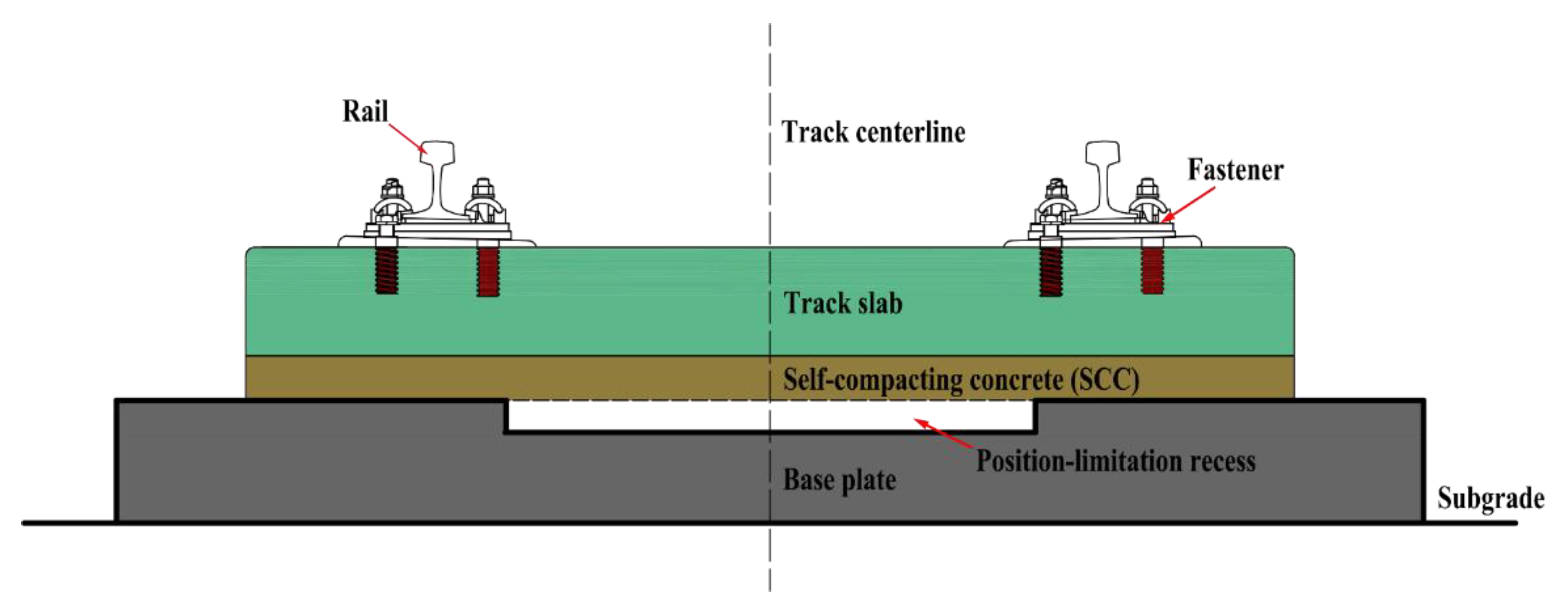
2. Temperature Field Fitting and Simulation of CRTS III Slab Track

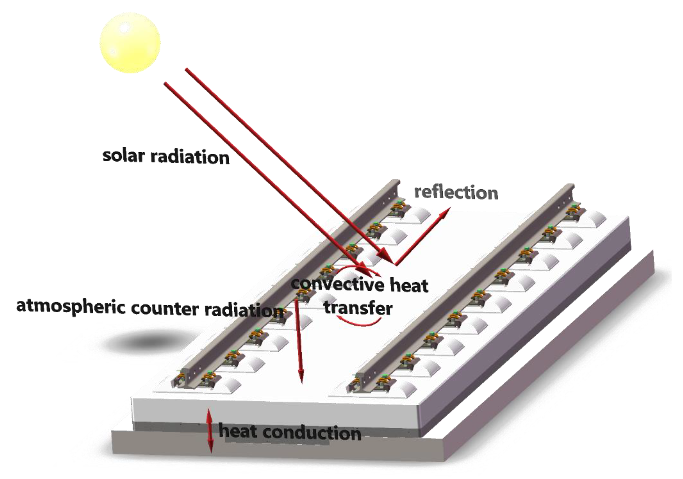
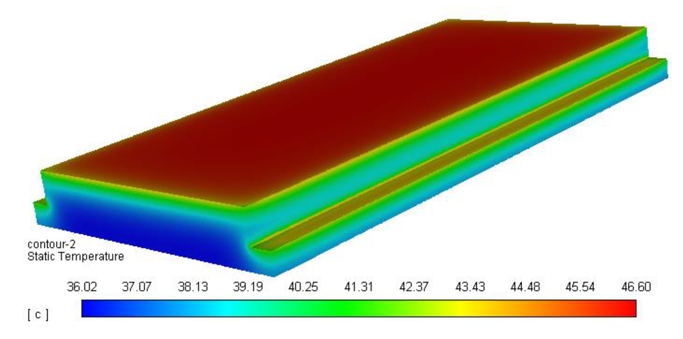
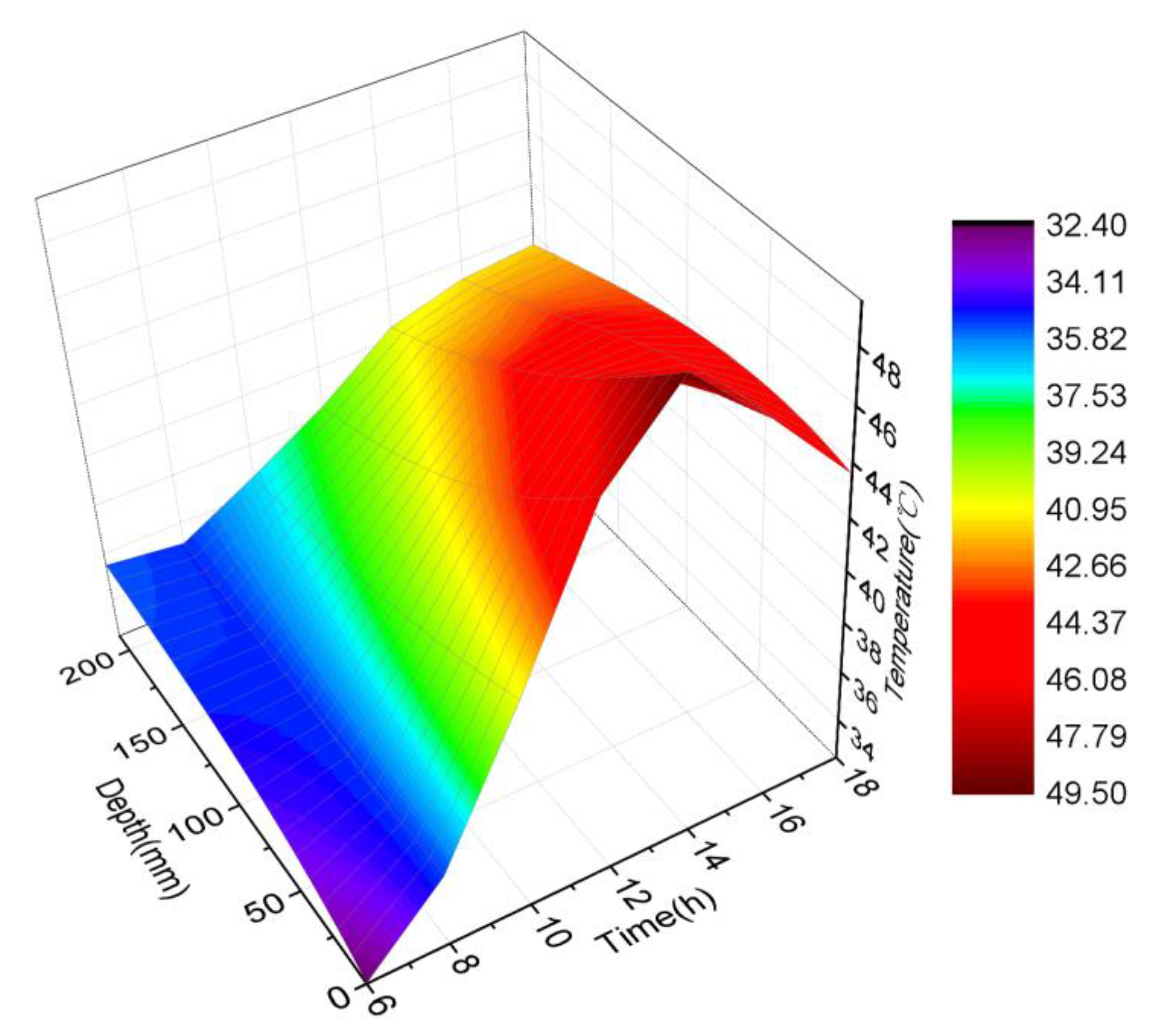
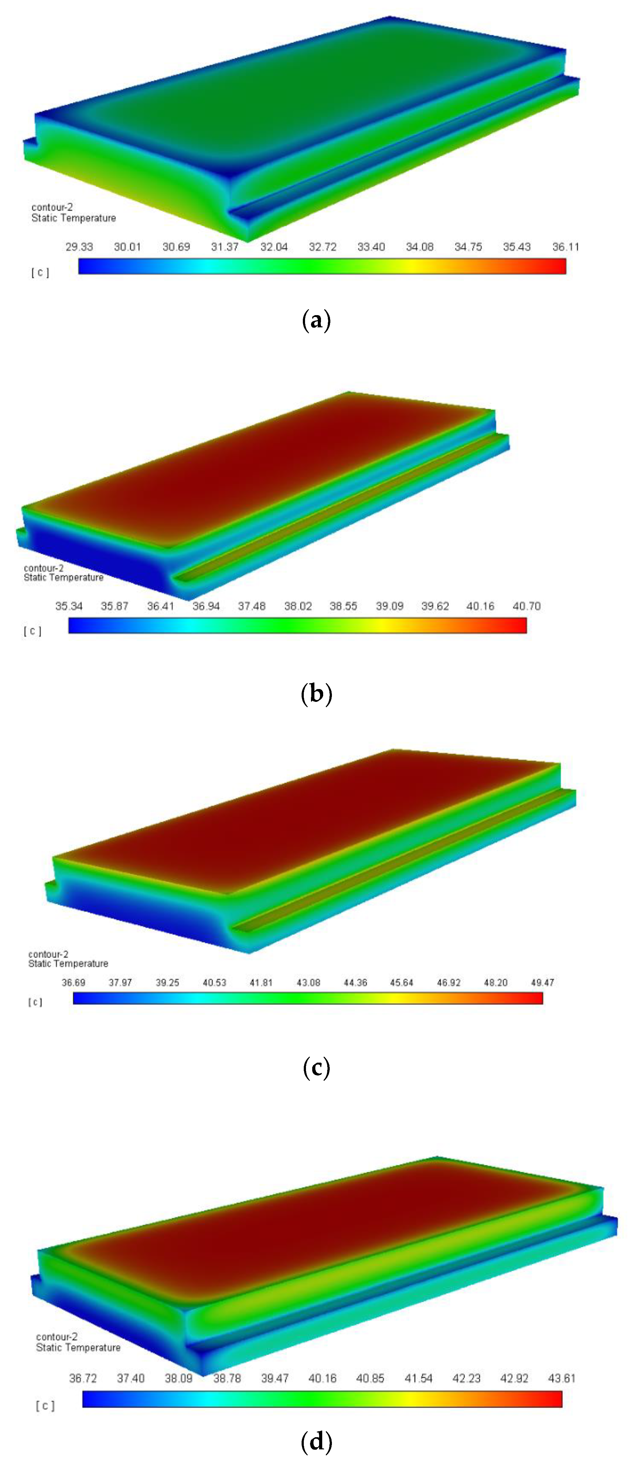
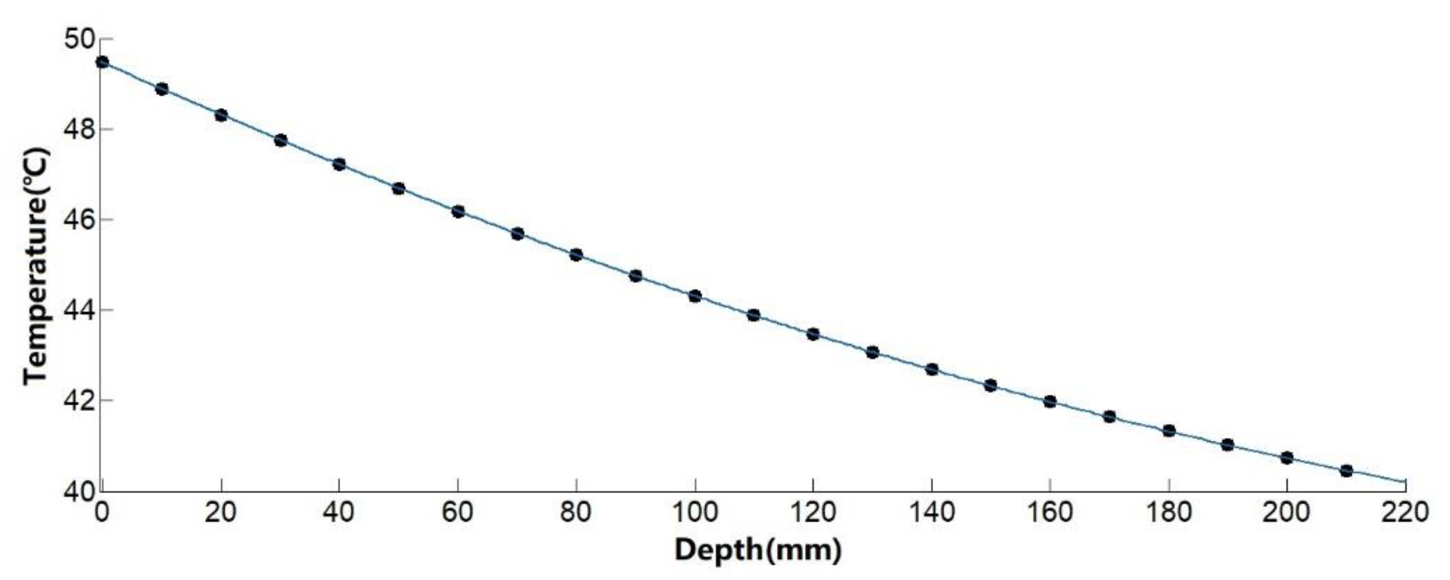
2.1. Temperature Field Fitting

In general, there are three methods of heat transfer: convective heat transfer, heat radiation, and heat conduction. For slab ballastless track, the temperature field inside the slab is affected by solar radiation and ambient temperature, that is, the convective heat transfer of air above the slab, solar radiation, and the self-balance and transfer of temperature inside the slab. Figure 2 is a schematic diagram of the heat exchange process of the ballastless track. The adjacent CRTS III slab tracks are not directly connected. There is a gap between the two slab tracks, and the mutual heat transfer can be ignored; therefore, only one of them was the focus of this study.

The Newtonian cooling equation is used to describe convective heat transfer:

$$q^{″}=h\left(T_s-T_B\right)$$

(1)

where h is the convective heat transfer coefficient, which is related to the surface shape, air temperature, and other factors. T_S is the surface temperature of the slab track and T_B is the ambient air temperature.

According to the literature [5], the atmospheric radiation on a sunny day can be calculated by the following formula:

$$G_a={\epsilon }_a{C}_0{\left(273+T_a\right)}^4$$

(2)

where ${\epsilon }_a$ is the atmospheric radiation coefficient, C₀ is the Stefan–Boltzmann constant, and T_a is the effective temperature, °C.

Combined with the internal temperature field distribution of slab ballastless track, the basic law of heat conduction is

$$\frac{Q}{t}=\frac{KA\left(T_{hot}-T_{cold}\right)}{d}$$

(3)

where Q is the total heat transfer in time period t, K is the heat conductivity, T is the temperature, A is the area of the plane, and d is the area between the two planes.

The model was established according to the dimensional parameters shown in

Table 1. Dimensional parameters of CRTS III slab track.

	Length (mm)	Width (mm)	Height (mm)
Slab track	5600	2500	210
Self-compacting Concrete	5600	2500	100
Base plate	5600	2900	200

. The density of the slab track is 2500 kg/m³, the heat transfer coefficient is 4.74 W/(m²·K), the specific heat capacity is 960 J/(kg·K), and the thermal conductivity is 1.75 W/(m·K). The density of self-compacting concrete is 2450 kg/m³, and the density of the base plate is 2500 kg/m³. The model ignores the influence of rails and fasteners on the temperature of the slab track and the influence of solar radiation on the surroundings of the slab track.

The solar direction vector, direct normal solar radiation from the earth’s surface, diffuse solar radiation from the vertical and horizontal surface, and ground reflection solar radiation are calculated by the calculation module in the CFD software. This study used the slab track of a section of a high-speed railway in operation in China as an example. According to meteorological data, the temperature in this area reaches its highest around 15 August every year. To explore the temperature gradient and deformation of the slab track under extreme conditions, the model was developed to simulate and calculate the temperature field distribution of the slab track in this section on 15 August.

The slab ballastless track is mainly exposed to solar radiation on the surface of the slab. Due to the rotation of the sun, the four sides of the slab will receive direct sunlight at different times, and the area around the slab is small and will not receive solar radiation all the time. To simplify the model, the influence of solar radiation around the model was not considered in the calculation. The boundary conditions around the model mainly consider heat conduction and convective heat transfer. The lower part of the base plate and the surface of the bridge conduct heat. Therefore, the boundary conditions mainly consider heat conduction. In the model, not only the influence of heat conduction and radiation on the upper surface and both sides of the base plate but also the influence of solar radiation on the temperature of the slab track are considered. Since the CFD software used can only load solar radiation energy on semi-transparent or transparent boundary conditions and cannot directly load solar radiation on opaque walls, it needs to use Stefan-Boltzmann’s law, Formula (4) to calculate the need to load the temperature of radiation [26]:

$$q_{rad}=\sigma \epsilon \left(T_{\max }^4-T_{\min }^4\right)$$

(4)

where $\sigma$ is the Stefan–Boltzmann constant, with a value of 5.6704 × 10⁻⁸ W/(m²·K⁴), and $\epsilon$ is the surface emissivity of the object, also known as the degree of blackness.

The temperature field model of ballastless track was used to calculate the temperature field under solar radiation in the daytime in mid-August. As shown in Figure 3, the temperature of the track surface under the influence of solar radiation reached 46.6 °C at 12:00. The temperature around and at the bottom of the slab track is about 41 °C. It can be seen that the temperature of the base plate does not change much. Solar radiation causes the surface temperature of the slab track to rise rapidly and the slab track has poor heat transfer capacity, resulting in a large temperature gradient inside the slab track.

Figure 4 is a three-dimensional diagram of temperature changes inside the slab track during the daytime. It can be seen that there was a negative temperature gradient inside the slab track at 6:00. The temperature gradient inside the slab track was the smallest at 8:00. After 8:00, the surface temperature of the slab track rose rapidly, and the interior of the slab track showed a positive temperature gradient. The surface temperature of the slab track formed an obvious peak at 14:00. Overall, the slab track surface temperature variation is greater than the internal temperature variation.

To carry out the deformation simulation of the slab track, it was necessary to fit the internal temperature field of the slab track. The temperature distribution at each time point in the daytime of the slab track in mid-August was calculated, and the results are shown in Figure 5.

To obtain specific temperature data for the follow-up study, the temperature data at different depths at the center of the slab track were exported and are shown in

Table 2. The vertical temperature at different positions in the center of slab track.

The Distance from Slab Track Surface(mm)	6:00 (°C)	8:00 (°C)	10:00 (°C)	12:00 (°C)	14:00 (°C)	16:00 (°C)	18:00 (°C)
0	32.424	35.28	40.696	46.601	49.475	46.725	43.606
10	32.802	35.26	40.404	45.97	48.887	46.655	43.778
20	33.141	35.242	40.122	45.366	48.314	46.545	43.91
30	33.442	35.225	39.852	44.79	47.757	46.396	44
40	33.709	35.209	39.592	44.242	47.216	46.213	44.052
50	33.945	35.195	39.343	43.721	46.692	45.999	44.067
60	34.153	35.182	39.105	43.226	46.183	45.76	44.05
70	34.337	35.17	38.878	42.757	45.691	45.5	44.002
80	34.498	35.159	38.661	42.312	45.216	45.222	43.927
90	34.64	35.149	38.454	41.891	44.756	44.93	43.828
100	34.765	35.141	38.258	41.494	44.313	44.627	43.706
110	34.876	35.134	38.071	41.118	43.886	44.317	43.565
120	34.973	35.129	37.894	40.763	43.474	44.002	43.408
130	35.06	35.124	37.726	40.429	43.079	43.685	43.236
140	35.137	35.121	37.567	40.115	42.699	43.367	43.051
150	35.206	35.118	37.418	39.819	42.335	43.051	42.857
160	35.269	35.117	37.277	39.541	41.985	42.739	42.654
170	35.325	35.117	37.144	39.281	41.651	42.432	42.445
180	35.376	35.119	37.02	39.036	41.332	42.13	42.231
190	35.422	35.121	36.903	38.807	41.027	41.836	42.015
200	35.465	35.124	36.794	38.593	40.735	41.55	41.796
210	35.505	35.129	36.692	38.392	40.458	41.273	41.578

.

The fitting toolbox in MATLAB was used to fit the temperature data. Generally speaking, the higher the order of the function in the fitting equation, the better the fitting effect, but the corresponding solution cost is also higher. Through calculation and comparison, it was found that the fitting of the cubic function of the slab track depth and temperature at 6:00 can achieve high accuracy, as shown in Figure 6. The fitting function is as follows:

$$\begin{array}{l}y=0.00000033x^3-0.0001812x^2\\ +0.03818x+32.44,R^2=0.9999\end{array}$$

(5)

The relationship between the slab track depth and the temperature at 14:00 can be achieved with high accuracy by quadratic function fitting, as shown in Figure 7. The fitting function is

$$\begin{array}{l}y=0.00007895x^2-0.05944x+\\ 49.47,R^2=1\end{array}$$

(6)

Using the same method, the temperature data under various working conditions were fitted to provide a basis for the subsequent solution of the temperature load applied in the displacement of the slab track.

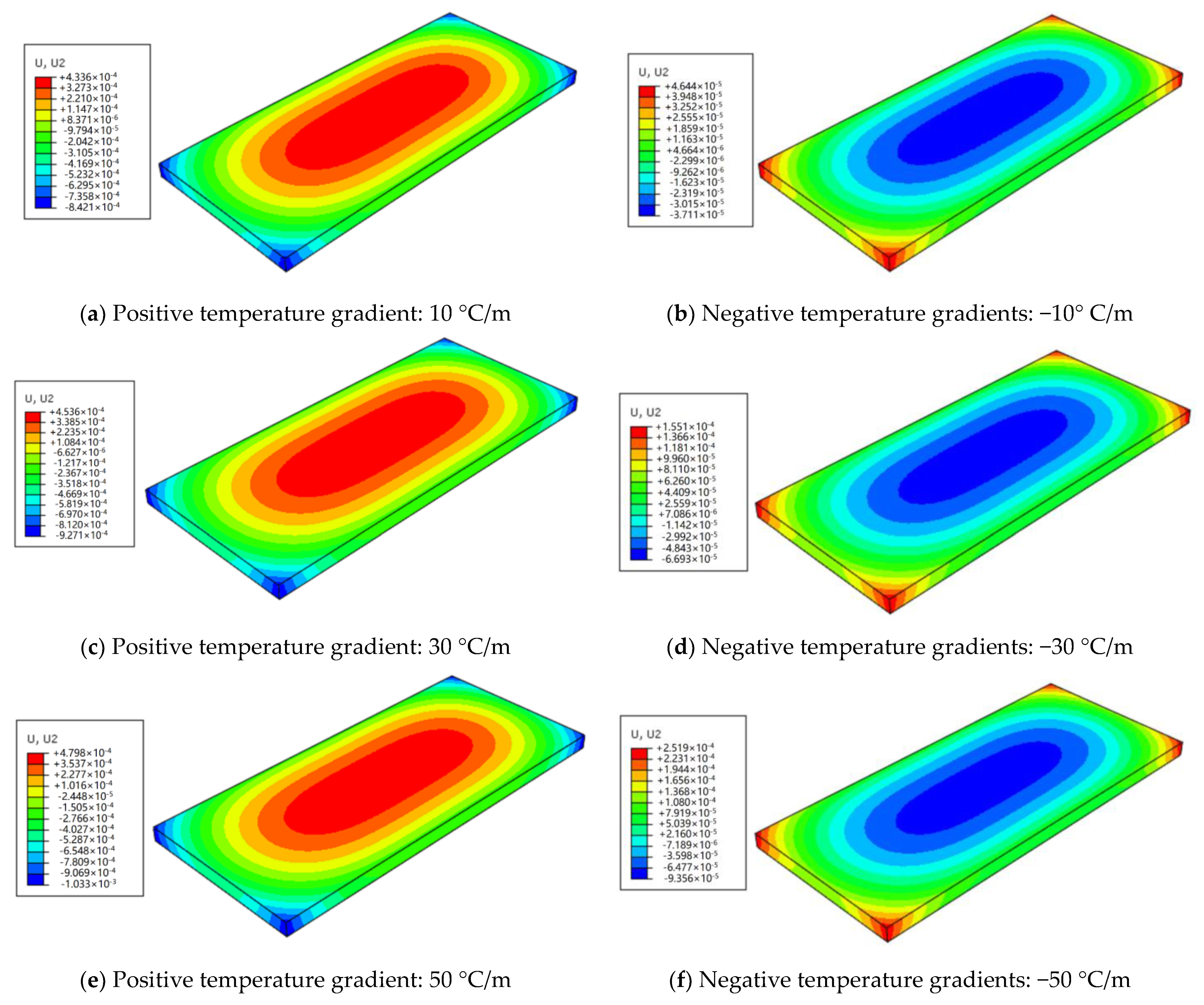
2.2. Simulation Analysis of CRTS III Slab Track Deformation

The research on the thermal stress of an object is the process of obtaining the stress and strain of the object by knowing the temperature distribution inside the object. In this study, finite element software was used to fit the data results of the temperature field obtained by simulation. The vertical temperature load distribution of the slab track was applied according to the function formula fitting the relationship between the temperature and the slab track depth in MATLAB. The temperature division of the slab track model is shown in Figure 8.

The temperature field of sequential coupling thermal stress determines the stress and strain field in the analysis, and the stress and strain field does not affect the temperature field. The obtained stress and strain field was used as a known condition for thermal stress analysis. The stress–strain simulation model of the ballastless track was established according to the parameters shown in

Table 3. Thermodynamic parameters of the ballastless track displacement simulation model.

Material	Properties
Fail	Linear expansion coefficient: 1.2 × 10−5/°C Elastic modulus: 2.1 × 1011 pa Density: 7850 kg/m3 Poisson ratio: 0.3
Fastener	Vertical stiffness: 50 kN/mm Transverse stiffness: 35 kN/mm Fastener spacing: 0.65 m
Slab track	Linear expansion coefficient: 1 × 10−5/°C Elastic modulus: 3.6 × 1010 pa Density: 2500 kg/m3 Poisson ratio: 0.2
Self-compacting concrete (SCC)	Linear expansion coefficient: 1×10−5/°C Elastic modulus: 3.25 × 1010 pa Density: 2450 kg/m3 Poisson ratio: 0.2
Base plate	Linear expansion coefficient: 1 × 10−5/°C Elastic modulus: 3.25 × 1010 pa Density: 2500 kg/m3 Poisson ratio: 0.2

[27].

Based on the above parameters, the stress–strain simulation model of ballastless track was established, and a slab was selected for stress and strain analysis. The size parameters of the model have been given. In the stress–strain simulation model of ballastless track, the rail mesh size is 200 mm. The mesh sizes of slab track, self-compacting concrete, and base plate are 50 mm. In the established finite element model, the lower surface of the slab track is bound to the upper surface of the self-compacting concrete, and the lower surface of the self-compacting concrete is bound to the upper surface of the base plate. The foundation can be divided into three types: elastic foundation, plastic foundation, and elastic–plastic foundation. The foundation under the ballastless track base plate is an elastic foundation. The model uses the grounding spring to simulate the ballastless track foundation, and its supporting stiffness is 76 MPa/m. The initial temperature of the model is set at 25 °C. Ballastless track is generally subjected to an overall temperature load and a positive/negative temperature gradient load. The temperature rise and fall of the track structure will lead to the expansion or contraction of the slab track, and the temperature gradient will cause warping deformation of the slab track. The combined action of the two cases may lead to varying degrees of deformation of the slab track.

Table 4. Displacement changes in the middle of the slab track and the edge of the slab during the overall heating and cooling.

		Displacement Variation in the Middle of Slab/mm	Displacement Variation of the Edge of the Slab/mm
Heating	10 °C	0.032	0.035
	20 °C	0.083	0.086
	30 °C	0.134	0.137
	40 °C	0.185	0.188
Cooling	10 °C	−0.07	−0.067
	20 °C	−0.121	−0.118
	30 °C	−0.172	−0.169
	40 °C	−0.223	−0.22

shows the displacement changes in the middle and corner of the slab under the conditions of heating and cooling. It can be seen that the displacement of the slab is positive due to the thermal expansion of the slab during heating. The displacement variation at the edge of the slab is greater than that at the middle of the slab. When the overall temperature is lowered, the slab track shrinks due to the lowering of the temperature, and the displacement is all negative. The displacement in the middle of the slab is slightly larger than at the edge of the slab.

Table 5. Displacement changes in the middle and edge of the slab track under positive and negative temperature gradients.

		Displacement Variation in the Middle/mm	Displacement Variation of the Edge/mm
Positive temperature gradient	10 °C/m	0.428	−0.781
	30 °C/m	0.453	−0.873
	50 °C/m	0.477	−0.981
Negative temperature gradient	−10 °C/m	−0.035	0.0464
	−30 °C/m	−0.061	0.155
	−50 °C/m	−0.085	0.252

and Figure 9 are the simulation results of vertical displacement of the slab track under a positive temperature gradient and a negative temperature gradient. In Table 5, the center position is the geometric center of the upper surface of the slab track. The edge position is the quadrilateral vertex on the upper surface of the slab track in the model. It can be seen that under the effect of a positive temperature gradient, the middle part of the slab deforms upward, and the edge of the slab deforms downward. The downward displacement of the middle of the slab is the largest under the action of the negative temperature gradient. An elliptical area is formed in the middle. The more outward the displacement, it gradually changes from downward to upward.

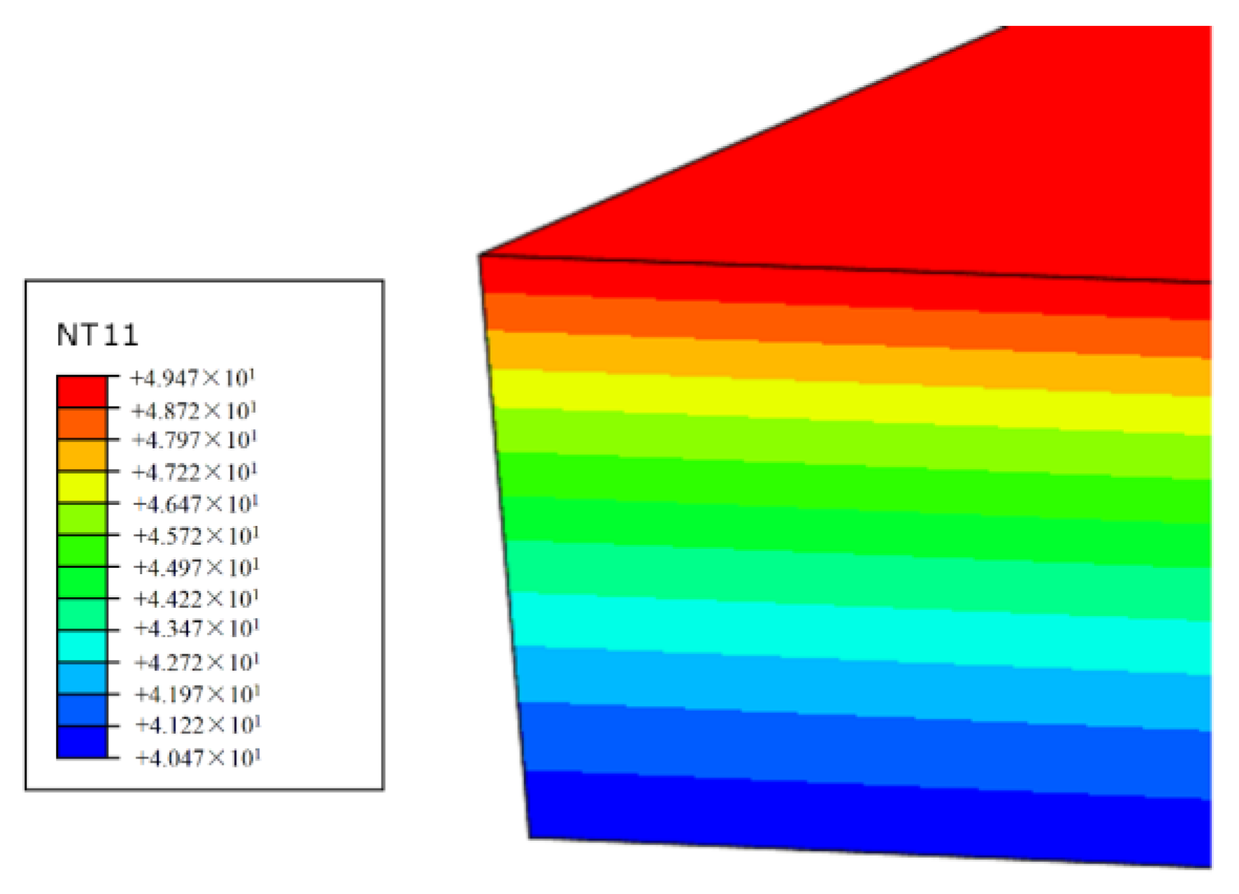
3. Verification of CRTS III Slab Track Deformation Simulation Model

At present, there are few field tests on the deformation of CRTS III slab track. To verify the accuracy of the simulation model established in this paper, the slab track of a high-speed railway under operation was selected for a field test. The test section was a straight section, the slab was on the elevated and simply supported box girder section, and the three slab tracks were located in the middle of the bridge. The test area was surrounded by farmland and there were no buildings. The displacement sensors and temperature sensors selected for the experiment were demarcated and durability-tested to ensure the credibility of the collected data. The installation of the sensors is shown in Figure 10; two contact displacement sensors (LVDT) were installed at each displacement measuring point, with a total of 20 sensors. The temperature sensors were installed in the middle of the slab, with depths of 20 mm, 100 mm, and 180 mm, respectively, as shown in Figure 11. The installation of the sensors in the field test is shown in Figure 12.

According to the working conditions of the measured data, the input parameters of the model were ensured to be consistent with the measured working conditions of the selected date. The temperature field of the ballastless track in the daytime in mid-August was calculated by using the temperature field model of the ballastless track, and the temperature field simulation results of the slab track were obtained and compared with the measured data, as shown in Figure 13. The difference between the simulation results at each time point and the measured results is small, and the changing trend of the curve is the same. The calculation results of the ballastless track temperature field solving model can represent the overall temperature distribution of the slab track.

At the same time, to verify the accuracy of the ballastless track displacement simulation results, the simulation results were compared with the measured slab displacement results. The comparison between the measured and simulated results is shown in Figure 14. The simulation results are slightly less than the measured displacement of the slab track. This error may be mainly caused by the following factors: When the temperature load in the slab track was applied, the calculated entire temperature field was not imported into the ballastless track stress–strain model. The stress–strain model of the ballastless track does not consider the setting of the internal steel reinforcement, and there is no prestressing force in the ballastless track. The displacement difference between the simulation results and the measured results in the middle of the slab is 0.015 mm, and the trend of the simulation results and the measured results is the same. In high-temperature weather, the middle of the slab track was deformed upward, and the edge of the slab was deformed downward. Therefore, the stress–strain model of the ballastless track can be used to study the deformation trend and deformation process of the slab track under temperature loads.

In summary, the stress–strain model of CRTS III slab ballastless track developed in this study can reflect the temperature field inside the slab track and the vertical displacement of the slab track at the macro-level under the condition of meeting the accuracy requirements. According to the simulation results, combined with meteorological conditions, it can provide technical data for the maintenance and repair of CRTS III slab track, focusing on targeted maintenance and repair.

4. Discussion and Future Works

Through the modeling and simulation of CRTS III slab ballastless track, the temperature field inside the slab track and the vertical displacement of the slab track reflected in the macro level was simulated, and the model was verified by field test. The results of the model simulation and the field test are comparable. When the temperature gradient was positive, the central part of the slab track deformed upward and the edge of the slab track deformed downward. The displacement in the central part of the slab track was the largest and the elliptical region was formed in the middle. The more outward the displacement was, the smaller the displacement was. When the temperature gradient was negative, the downward displacement in the middle of the slab track was the largest, an elliptical region was formed in the middle, and the outward displacement gradually changed from downward to upward. The model established in this study can accurately reflect the temperature field inside the slab track and the vertical displacement of the slab track at the macro level. In practical application, the technical data can be provided for the maintenance of CRTS III slab track according to the simulation results. The temperature field distribution and possible deformation of the slab track can be obtained by adding working condition simulation conditions according to climatic conditions. These predictions can be used to focus on targeted maintenance and repair.

Our sensors are still installed on the CRTS III slab ballastless track. We will conduct long-term monitoring of the CRTS III slab ballastless track. The simulation research is not limited by the field test conditions, and can obtain the required data more conveniently. However, simulation research cannot replace field testing. Therefore, in future research, we will combine the measured data to continuously optimize and improve the simulation model, improve the accuracy of the model, and provide basic data for maintenance.

References

1. Yang, C.; Wu, C.L.; Liu, D.Y. The illumination of Tokaido Shinkansen for China’s high-speed rail development. Planners 2016, 32, 136–141. [Google Scholar]
2. Gao, Q.; Zhou, C. Contrasted analysis of the comprehensive performances of CRTS series ballastless tracks on high-speed railway. J. Shandong Agric. Univ. Nat. Sci. 2019, 50, 236–239. [Google Scholar]
3. Schindler, A.K.; Ruiz, J.M.; Rasmussen, R.O.; Chang, G.K.; Wathne, L.G. Concrete pavement temperature prediction and case studies with the FHWA HIPERPAV models. Cem. Concr. Compos. 2004, 26, 463–471. [Google Scholar] [CrossRef]
4. Potgieter, C.; Gamble, W. Nonlinear temperature distributions in bridges at different locations in the United State. PCI J. 1989, 34, 81–103. [Google Scholar] [CrossRef]
5. Kehlbeck, F.; Liu, X.F. The Influence of Solar Radiation on the Bridge Structure; China Railway Publishing House: Beijing, China, 1981. [Google Scholar]
6. Zheng, Y.X.; Cai, Y.C.; Zhang, Y.M. Study on temperature prediction model of asphalt concrete pavement. Adv. Mat. Res. 2011, 243–249, 506–509. [Google Scholar] [CrossRef]
7. Wu, J.X. Characteristics and temperature test technology of CRTS II ballastless track on bridge. Chin. Overseas Archit. 2015, 3, 138–140. [Google Scholar]
8. Sun, Z.J.; Wang, Z.P.; Wang, J.; Kang, W.X.; Liu, X.Y. Temperature analysis of CRTS II slab ballastless track in extremely hot weather. Railw. Stand. Des. 2018, 62, 64–68. [Google Scholar]
9. Wu, B.; Liu, C.; Zeng, Z.P.; Wei, W. Research on the temperature field characteristic of CRTS II slab ballastless. J. Railw. Eng. Soc. 2016, 33, 29–33. [Google Scholar]
10. Liu, Y.; Chen, P.; Zhao, G.T. Study on characteristics of early temperature field of CRTS II slab ballastless track structure. China Railw. Sci. 2014, 35, 1–6. [Google Scholar]
11. Liu, Y. Study on Characteristics and Influences of CRTS II Slab Track Early Temperature Field. Ph.D. Thesis, Southwest Jiaotong University, Chengdu, China, 2013. [Google Scholar]
12. Barber, E.S. Calculation of maximum pavement temperatures from weather reports. Highw. Res. Board Bull. 1957, 168, 1–8. [Google Scholar]
13. Williamson, R.H. Effects of environment on pavement temperatures. In Proceedings of the 3rd International Conference on Structural Design of Asphalt Pavements, London, UK, 1–4 September 1972; pp. 144–158. [Google Scholar]
14. Hall, F.L.; Barrow, D. Effect of weather and the relationship between flow and occupancy on freeways. Transp. Res. Rec. 1988, 1194, 55–63. [Google Scholar]
15. Robertson, W.D. Determining the winter design temperature for asphalt pavement. In Proceedings of the Asphalt Paving Technology 1997, Salt Lake City, UT, USA, 17–19 March 1997; pp. 312–343. [Google Scholar]
16. Huber, G.A. Weather Database for the Superpave (Trademark) Mix Design System; National Research Council: Washington, DC, USA, 1994; Volume 2, p. 143. [Google Scholar]
17. Mohseni, A.; Symons, M. Improved AC pavement temperature models from LTPP seasonal data. In Proceedings of the Transportation Research Board 77th Annual Meeting, Washington, DC, USA, 11–15 January 1998; pp. 71–72. [Google Scholar]
18. Kennedy, T.W.; Huber, G.A.; Harrigan, E.T.; Cominsky, R.J.; Hughes, C.S. Superior Performing Asphalt Pavements (Superpave): The Product of the SHRP Asphalt Research Program; National Research Council: Washington, DC, USA, 1994; pp. 150–156. [Google Scholar]
19. Liu, X.Y.; Zhao, P.R.; Yang, R.S.; Wang, P. Theory and Method of Ballastless Track Design for Passenger Dedicated Line; Southwest Jiaotong University Press: Chengdu, China, 2010. [Google Scholar]
20. Yang, J.J.; Zhang, N.; Gao, M.M.; Sun, J.L. Temperature warping and its impact on train-track dynamic response of CRTS II ballastless track. Eng. Mech. 2016, 33, 210–217. [Google Scholar]
21. Yang, J.J. Temperature Deformation of CRTS II Track Slab and Its Impact on Dynamic Response of Vehicle-Track-Bridge System. Ph.D. Thesis, Beijing Jiaotong University, Beijing, China, 2017. [Google Scholar]
22. Wei, J.; Ban, X.; Dong, R.Z. Analysis of effects and damage of CRTS II ballastless track structure system induced by temperature. J. Wuhan Univ. Technol. 2012, 34, 80–85. [Google Scholar]
23. Ban, X. Analysis of the Performance of CRTS II Slab Ballastless Track Structure under Temperature. Master’s Thesis, Central South University, Changsha, China, 2012. [Google Scholar]
24. Yi, T.B.; Zhao, Q.J.; Xiao, W. Analysis of temperature deformation and stress value of CRTS I track slab on Harbin-Dalian passenger dedicated line. Railw. Stand. Des. 2012, 5, 37–40. [Google Scholar]
25. Zhao, Y.; Si, D.L.; Jiang, Z.Q.; Wang, J.J.; Li, H. Study on temperature field and deformation of CRTS I slab-type ballastless track in severe cold area. Railw. Eng. 2016, 05, 47–52. [Google Scholar]
26. Wen, Z. Application Tutorial of Fluent Fluid Calculation; Tsinghua University Press: Beijing, China, 2009. [Google Scholar]
27. Tan, X. Study on Mechanical and Deformation Characteristics of CRTS III Slab Ballastless Track under Complicated Temperature. Master’s Thesis, Beijing Jiaotong University, Beijing, China, 2018. [Google Scholar]
Figure 1. Schematic diagram of the CRTS III slab ballastless track structure.
Applsci 11 07830 g001
Figure 2. Schematic diagram of the heat exchange process of the ballastless track.
Applsci 11 07830 g002
Figure 3. Simulation results of the ballastless track temperature (12:00).
Applsci 11 07830 g003
Figure 4. Diagram of simulation results of temperature variation with time at different depths during the daytime.
Applsci 11 07830 g004
Figure 5. The overall temperature distribution of the slab track at each time. ((a).6:00, (b).10:00, (c).14:00, (d).18:00).
Applsci 11 07830 g005
Figure 6. The cubic function fitting results of the relationship between the slab track depth and the temperature at 6:00.
Applsci 11 07830 g006
Figure 7. The quadratic function fitting results of the relationship between the slab track depth and the temperature at 14:00.
Applsci 11 07830 g007
Figure 8. The temperature division of the slab track.
Applsci 11 07830 g008
Figure 9. Simulation results of vertical displacement of slab track under positive and negative temperature gradients.
Applsci 11 07830 g009
Figure 10. The schematic diagram of the sensors’ positions.
Applsci 11 07830 g010
Figure 11. Diagram of the installation positions of the temperature sensors.
Applsci 11 07830 g011
Figure 12. The installation of sensors for the field test.
Applsci 11 07830 g012
Figure 13. Comparison between the simulation and measurement results of the slab track temperature.
Applsci 11 07830 g013
Figure 14. Comparison of measured displacement and simulation results of slab track.
Applsci 11 07830 g014