Comparison of Nonlinear and Linear Controllers for Magnetic Levitation System

Abstract

Nonlinear system control belongs to advanced control problems important for real plants control design. Various techniques have been developed in this field. In this paper we compare two different approaches to a nonlinear unstable Magnetic levitation system control. The first control design approach further develops our recent results on robust discrete-time pole-placement, based on convex D_R-regions. The second studied approach is based on feedback linearization and the simplified development of the corresponding nonlinear control law is provided. Both approaches are compared and evaluated. The efficiency of robust discrete-time pole-placement controller is shown as well as its competitiveness in comparison with nonlinear control for Magnetic levitation system.

1. Introduction

In practice, a control is designed mostly for nonlinear systems, various nonlinear control approaches have been developed during past decades (sample of excellent books on nonlinear control is [1,2]). Nevertheless, some kind of linearization is frequently used to simplify analysis and control design of inherently nonlinear systems. Techniques based on feedback linearization can be used under certain, not too strict assumptions on nonlinear system, see e.g., [3,4]. The resulting control design scheme then provides a nonlinear control law which can be designed based on a transformed linearized closed-loop control system. Other possibility to control a nonlinear system is to use a linearized uncertain model or its parameter varying (LPV) alternative and design a corresponding robust, adaptive or gain scheduling control. A nice survey of robust control techniques is in [5], gain scheduling approach can be found in [6].

Among various robust control techniques, Linear Matrix Inequality (LMI) approach attracted notable interest owing to its computational tractability [7,8,9,10]. Specifically, when a polytopic uncertain linear model is used, different robust control algorithms can be formulated in LMI framework, as $H_{inf}$, $H_2$, LQG (Linear–Quadratic–Gaussian) based controllers and other robust controllers designed using quadratic or parameter dependent Lyapunov function [8,10,11]. Successful control design has to meet basic requirements on closed-loop stability and performance. For uncertain system, stability and prescribed performance is required for the whole uncertainty domain. One of the frequently used approaches to guarantee the prescribed closed-loop system dynamics is pole-placement technique [7,12,13,14,15] and others. In pole-placement, it can be advantageous to prescribe only a region, where the closed-loop poles should be placed instead of their exact position. Such approach is especially useful for robust control of uncertain systems. An appropriate region can be determined by the prescribed settling time, overshoot, stability degree, relative damping or other performance indices closely connected with closed-loop pole position [12,13,14]. In this field, so called $D_R$ region concept have been introduced and used for robust control design [7,9,10,16], where $D_R$ region is a convex domain in a complex plane, where the system poles should lie. The corresponding $D_R$ stability condition in the form of LMI, provides computationally efficient way for the respective controller design. The existing results in literature have been mostly proposed for continuous-time systems [10,14,15,17]. In our recent works [18,19,20] we developed specific $D_R$ regions for discrete-time systems, motivated by the fact that in real world application, mostly the digital controllers are implemented. In this paper we aim at the comparison of our recent results on robust pole-placement discrete-time state feedback control design with a nonlinear control developed for a laboratory magnetic levitation (ML) plant.

Magnetic levitation principle is widely used in applications, besides transport systems (as Maglev train) also magnetic bearings, frictionless contacts, microrobotics and others. Magnetic levitation plant, where a magnetic object is positioned in the air space, provides a challenging control task owing to strong nonlinearity and inherent instability. Various methods have been proposed to control the magnetic levitation, as for example feedback linearization approach in [21,22], adaptive state feedback [23], frequency domain method [24] or CDM (Coefficient Diagram Method) based design in [4]. Most of them consider continuous-time control. In [18,19,20] we proposed $D_R$ region based discrete-time robust pole-placement controller for ML system.

This paper is devoted to a study and comparison of two principal approaches applied on a laboratory Magnetic levitation system. The first approach is based on feedback linearization [3,4,22], where an algebraic transformation is applied on nonlinear state space model together with a nonlinear control law to obtain the linearized closed-loop system. The second approach employs robust pole-placement controller design for a system linearized around the working point and described by an uncertain polytopic system [7,9,18,19]. The main contribution of the paper is in simplified development of nonlinear control law with novel approximation of nonlinear terms, developed robust pole-placement controller for different levitating balls, comparison and evaluation of the obtained results received with nonlinear continuous-time control and discrete-time linear one. The advantages and disadvantages of both used approaches are summarized for the studied case.

The paper is structured as follows. Section 2 describes the Magnetic levitation plant, its nonlinear model and parameters. Section 3 is devoted to state feedback control design, two approaches are presented, Section 3.1 recalls our recent results on a discrete-time $D_R$ region based controller design, in Section 3.2, nonlinear control law is developed following the concept introduced in [22]. Section 4 presents designed controllers for Magnetic levitation, the discrete-time robust pole-placement controllers in Section 4.1 and continuous-time nonlinear controller in Section 4.2. Comparison and assessment of the designed controllers is provided in Section 4.3, paper contribution is briefly summarized in Conclusion.

2. Nonlinear Magnetic Levitation System

This paper studies and compares control designs for Magnetic levitation laboratory plant (ML), Figure 1. Magnetic levitation is inherently unstable system with fast dynamics corresponding to electromagnetic forces [19,25]. In our laboratory plant, the aim is to position the levitating ferromagnetic ball (sphere) within the air-space between two electromagnets. Below, we consider the upper coil serving as an actuator which compensates gravitation of the ball.

The ML nonlinear model below can be derived using Lagrange function. More details can be found in [26]. We omit argument t to improve readability. For the readers convenience we recall the basic steps of the development. Lagrange function (the difference between kinetic and potential energy) T is used in the form

$$T=\frac{1}{2}m{\left(\frac{dx}{dt}\right)}^2+\frac{1}{2}L\left(x\right){\left(\frac{dq}{dt}\right)}^2+\frac{1}{2}{\int }_0^{t}R{\left(\frac{dq}{dt}\right)}^{2}dt+mgx+qu$$

(1)

where x is a distance of the sphere from electromagnet (position), q is electric charge, m is a mass of the sphere, R is a resistance of the electromagnet coil, $L\left(x\right)$ is dependence of inductance of the coil on x, $I=dq/dt$ is a current in the coil, g is acceleration of gravity, u is voltage on the coil. From Lagrange equations, the following equations are obtained

$$\begin{array}{cc}\hfill \frac{d^{2}x}{d{t}^2}& =\frac{1}{2m}\frac{dL}{dx}{I}^2+g\hfill \\ \hfill \frac{dI}{dt}& =\frac{1}{L}\left(-\frac{dL}{dx}\frac{dx}{dt}I-RI+u\right).\hfill \end{array}$$

(2)

For inductance L, the next approximation is used

$$\frac{dL}{dx}=-a{L}_{1}exp(-ax)$$

(3)

The term $\frac{dI}{dt}$ is approximated by experimentally received expression

$$\frac{dI}{dt}=\frac{1}{f_1\left(x_1\right)}(k_{1}u+c_1-I),$$

(4)

$k_1,c_1$ can be directly measured, $f_1\left(x_1\right)$ is approximated analogically to (3). Substituting (3) and (4) into (2), splitting the first equation from (2) into two first order equations and introducing denotation

$$a\approx \frac{1}{F_{emP2}},L_1\approx F_{emP1},\frac{dL}{dx}\approx -\frac{F_{emP1}}{F_{emP2}}exp(-\frac{x_1}{F_{emP2}}),$$

the nonlinear ML model (5) is obtained

$$\begin{array}{cc}\hfill \frac{d{x}_1}{dt}& =x_2\hfill \\ \hfill \frac{d{x}_2}{dt}& =-\frac{F_{em1}}{2m}+g\hfill \\ \hfill \frac{d{x}_3}{dt}& =\frac{1}{f_1\left(x_1\right)}(k_{1}u+c_1-x_3)\hfill \end{array}$$

(5)

where

$$F_{em1}=x_3^2\frac{F_{emP1}}{F_{emP2}}exp(-\frac{x_1}{F_{emP2}}),f_1\left(x_1\right)=\frac{f_{1P1}}{f_{1P2}}exp(-\frac{x_1}{f_{1P2}}),$$

state variables are: $x_1=x$—position of the ball, $x_2$—velocity of the ball, $x_3=I$—current in the upper electromagnet coil, control input u is the voltage on the upper coil, output is the position of the ball $x_1$ measured as a distance from the upper coil.

Values for $F_{emP1},F_{emP2},f_{1P1},f_{1P2},k_1,c_1$ are inherent plant parameters, their values are specific for the concrete coil; see

Table 1. ML plant parameters used in nonlinear state model.

Parameters	Values	Units
m	0.016; 0.023; 0.039	kg
g	9.81	m/s2
$F_{emP1}$	0.017521	H
$F_{emP2}$	0.0058231	m
$f_{1P1}$	1.4142 $\times {10}^{-4}$	ms
$f_{1P2}$	4.5626 $\times {10}^{-3}$	m
$c_1$	−0.4	A
$k_1$	4.4	A
$i_{MIN}$	0.03884	A
$i_{MAX}$	2.38	A
$u_{MIN}$	0.00498	MU

for the considered ML.

All parameters are summarized in Table 1. The mass of the ball is 0.016 kg for the small ball, 0.023 kg for the medium ball and 0.039 kg for the big ball.

3. Control Design

A nonlinear system control design frequently uses linearization techniques, which provide powerful tools to simplify analysis and design. The main idea behind linearization approaches is to apply appropriate transformation to the nonlinear system so that the simplified—linearized model is obtained, for which some of many existing control design methods can be used.

In this section, two different approaches to a nonlinear system control design are presented. The first one is based on the classic linearization approach using Taylor series (Jacobian) around the appointed working point. To guarantee stability around the working point, the resulting linearized model is then represented as a polytopic uncertain system. For such system model, we recall a robust pole region approach introduced in [9] and briefly summarize our recent results for a discrete-time domain [18,19]. Robust pole-placement control is designed directly in a discrete-time domain since control implementation uses digital controller. In the second part of this section a nonlinear continuous time control law motivated by [22] and based on feedback linearization is developed for magnetic levitation. Presented result further develops nonlinear control law from [22] and uses approximation of lumped exponential terms by a rational function to simplify the resulting control law. The main motivation is to compare these two approaches and assess the qualities of recently developed, relatively simple robust pole-placement control [19].

3.1. Robust Pole Placement—Pole Region Approach

Robust control will be designed for a linearized model, considering three balls of different sizes and their corresponding masss.

The first step is to linearize the nonlinear model (5) around the determined working point using standard Jacobian method. In the following we will use the closed-loop response comparison for the position control of the ball at pos = 0.01 m. The resulting continuous-time linear state space model is:

$$\begin{array}{cc}\hfill \frac{dx}{dt}& =A_{c}x\left(t\right)+B_{c}u\left(t\right)=\left[\begin{array}{ccc}0& 1& 0\\ a_{21}& 0& a_{23}\\ 0& 0& a_{33}\end{array}\right]x\left(t\right)+\left[\begin{array}{c}0\\ 0\\ b_3\end{array}\right]u\left(t\right)\hfill \end{array}$$

$$y\left(t\right)=C_{c}x\left(t\right)=\left[\begin{array}{ccc}1& 0& 0\end{array}\right]$$

(6)

where

$a_{21}=\frac{1}{2m}\frac{F_{emP1}}{F_{emP2}^2}\left(x_{30}^{2}exp\left(-\frac{x_{10}}{F_{emP2}}\right)\right)$

$a_{23}=-\frac{x_{30}}{m}\frac{F_{emP1}}{F_{emP2}}\left(x_{30}^{2}exp\left(-\frac{x_{10}}{F_{emP2}}\right)\right)$

$a_{33}=-\frac{1}{f_i\left(x_{10}\right)}$

$b_3=k_1\frac{1}{f_i\left(x_{10}\right)}$

$x_{10}=pos$, $x_{20}=0$, $x_{30}=\sqrt{\left(\frac{2mg{F}_{emP2}}{F_{emP1}})\right)exp\left(-\frac{x_{10}}{F_{emP2}}\right)}$.

The control will be designed in discrete time domain, therefore, in the next step continuous time model (6) is discretized for appropriate sampling period $T_s=0.001$ s. Since we consider three different balls, the uncertain parameter corresponds to their mass m. The resulting discrete-time linearized model is then represented by a polytopic system (7) and (8), where the polytope vertices are obtained for different ball masses.

3.1.1. Robust Control Problem Formulation

Robust pole-placement controller is designed for a polytopic uncertain linear discrete-time dynamic system.

$$x(k+1)=A\left(\xi \right)x\left(k\right)+B\left(\xi \right)u\left(k\right),$$

(7)

where $x\left(k\right)\in R^n$ is the state vector, $u\left(k\right)\in R^m$ is the control input, $\xi \in R^N$ denotes the vector of uncertainty parameters corresponding to uncertainties belonging to the convex polytope described as follows

$$(A\left(\xi \right),B\left(\xi \right))\in \{\sum _{i=1}^N(A_i,B_i){\xi }_i,\sum _{i=1}^N{\xi }_i=1,{\xi }_i\ge 0\}$$

(8)

matrices $A_i,B_i$ are constant and have corresponding dimensions. It is assumed that all states can be used for feedback control

$$u\left(k\right)=Kx\left(k\right)$$

(9)

The control design goal is to find such feedback gain matrix K that the corresponding closed-loop system (10) is stable and conform to the prescribed performance limits, in our case it has all poles in the prescribed region in the convex plane.

$$x(k+1)=(A\left(\xi \right)+B\left(\xi \right)K)x\left(k\right)=A_{CL}\left(\xi \right)x\left(k\right).$$

(10)

3.1.2. $D_R$ Regions and $D_R$ Stability

Robust pole-placement belongs to efficient tools for uncertain system control design. So called $D_R$ region approach, introduced in [9] provides computationally tractable LMI condition which can be used for a robust controller design for uncertain polytopic systems. We start with definition of basic notions. A definition of $D_R$ region in the complex plain as set of points conforming to the specified matrix inequality is taken from [9].

$$D_R=\{z\in C:R_{11}+R_{12}z+R_{12}^T{z}^{*}+R_{22}z{z}^{*}<0\}.$$

(11)

To get convex formulation transformable to LMI, we assume that $R_{22}$ is positive definite (semidefinite). A generalized-$D_R$ stability notion can be defined for a specific $D_R$ domain determined for system poles. Matrix $A_{CL}(.)$ is said to be $D_R$ stable if and only if all its eigenvalues lie in the $D_R$ region defined by (11). Standard Lyapunov stability condition can be then generalized for the $D_R$ stability in the form of matrix inequality as summarized in the following lemma.

Lemma 1

([9]). Closed-loop matrix $A_{CL}\left(\xi \right)\in R^{n\times n}$ is $D_R$ stable if and only if there exists a positive definite matrix $P\left(\xi \right)\in R^{n\times n}$ such that

$$R_{11}\otimes P\left(\xi \right)+R_{12}\otimes \left(P\left(\xi \right)A_{CL}\left(\xi \right)\right)+R_{12}^T\otimes \left(A_{CL}{\left(\xi \right)}^{T}P\left(\xi \right)\right)+R_{22}\otimes \left(A_{CL}^T\left(\xi \right)P\left(\xi \right)A_{CL}\left(\xi \right)\right)<0.$$

(12)

It is important to note that the $D_R$ stability condition (12) can be for state feedback control directly converted to LMI which significantly reduces computational effort.

Standard domains for stable poles and matrices $R_{ij}$ defining the corresponding $D_R$ regions (11) can be listed as:

(I)

open left-half plane of the complex plane, $R_{11}=0,R_{12}=1,R_{22}=0$ (continuous-time systems),

(II)

interior of the unit circle, $R_{11}=-1,R_{12}=0,R_{22}=1$ (discrete-time systems),

(III)

shifted left-half plane of the complex plane corresponding to stability degree $\lambda$,

$R_{11}=2\lambda ,R_{12}=1,R_{22}=0$ (continuous-time systems),

(IV)

interior of the circle centered in [0, 0] with radius $r=1/sqrt\left(\alpha \right)$ corresponding to stability degree $sqrt\left(\alpha \right)$, $R_{11}=-1/\alpha ,R_{12}=0,R_{22}=1$ (discrete-time systems),

(V)

interior of the convex cone with vertex angle $2\phi$, corresponding to the relative damping (given by a ratio of the imaginary and real part of the complex pole in continuous-time systems)

$$R_{11}=R_{22}=\left[\begin{array}{cc}0& 0\\ 0& 0\end{array}\right],R_{12}=\left[\begin{array}{cc}sin\left(\phi \right)& cos\left(\phi \right)\\ -cos\left(\phi \right)& sin\left(\phi \right)\end{array}\right].$$

The domains (I) and (II) correspond to basic stability, domains (III) and (IV) to stability degree, which influences the speed of system response and also robustness, domain (V) determines the relative damping, belonging to important performance indices since it is related to oscillations of the system response. Recall that the stability degree defines the distance to the standard stability border, for continuous-time systems it given by the biggest real part of system poles—see (III); for discrete time system it is given by the inverse of radius of the circle where all system poles lie—see (IV).

3.1.3. Robust Pole-Placement Controller Design

Below, we recall the LMI formulation of $D_R$ stability condition for closed-loop uncertain system (12) which can be directly used to compute feedback gain matrix K for robust pole placement controller, more details can be found in [27].

Lemma 2

([9]). Consider the uncertain polytopic system with state feedback control (12). If there exist positive definite matrices $P_i\in R^{nxn}$ and any matrices $H\in R^{nxn}$, $S\in R^{mxn}$ such that the following inequality holds

$$\left[\begin{array}{cc}{M}_{11i}& M_{12i}\\ M_{12i}^T& M_{22i}\end{array}\right]<0i=1,...,N$$

(13)

where

$$\begin{array}{cc}\hfill M_{11i}& =R_{11}\otimes P_i+R_{12}\otimes (A_{i}H+B_{i}S)+R_{12}^T\otimes {(A_{i}H+B_{i}S)}^T\hfill \\ \hfill M_{22i}& =R_{22}\otimes (P_i-H-H^T)\hfill \\ \hfill M_{12i}& =R_{12}^T\otimes (P_i-H^T)+R_{22}\otimes (A_{i}H+B_{i}S),\hfill \end{array}$$

(14)

and the state feedback controller matrix is computed as

$$K=S{H}^{-1}.$$

(15)

then the closed-loop system (10) is $D_R$ stable for stability region (11).

Frequently, the integration term, or PI controller is required to eliminate the steady-state error of the controlled output variable. Then, the robust pole-placement controller design presented in Lemma 2 can be applied for the augmented state model which includes also the integration dynamics of PI controller. The augmented discrete-time system can be then described as

$$A_{i_{aug}}=\left[\begin{array}{cc}{A}_i& 0\\ C& I\end{array}\right],B_{i_{aug}}=\left[\begin{array}{c}{B}_i\\ 0\end{array}\right],i=1,\dots ,N$$

(16)

where matrix C corresponds to those outputs which are considered in the integration controller part. The state feedback gain matrix K is then in the following form

$$K=\left[\begin{array}{cc}{K}_p& K_I\end{array}\right],$$

(17)

matrices $K_p$ and $K_I$ correspond to proportional and integral gains of the PI controller. More details can be found in [27].

For the magnetic levitation system, the ball position is required to track the reference value, therefore in this case, the system output represented by the state $x_1$ enters the integration term and $C=\left[100\right]$.

In robust-pole placement, it is very important to appropriately prescribe the required closed-loop pole region. For ML we aim at achieving the determined stability degree and relative damping. The relative damping belongs to basic closed-loop (CL) performance requirements, however, in this case, the corresponding discrete-time region is no more convex, given by a logharitmic spiral and has a “cardioid” shape. This nonconvex region can be advantageously approximated using convex inner approximations which then enables controller design via LMI solution. Here, the inner ellipse and angle-ellipse approximations, which we developed recently [18,19] will be considered. The detailed description of considered pole regions is as follows.

(A) Standard Stabilizing Controller (Unit Circle)

In the first controller design, based on LMI approach, we will use a standard stabilizing controller from [28]:

$$\begin{array}{cc}\hfill \left[\begin{array}{cc}H+H^T-P_i& {(A_{i_{aug}}H+B_{i_{aug}}S)}^T\\ A_{i_{aug}}H+B_{i_{aug}}S& P_i\end{array}\right]& \ge 0\hfill \\ \hfill P_i>0,i=1,\dots ,N.\end{array}$$

(18)

the state feedback controller matrix is then computed by (15).

(B) Discrete-time Robust Pole-placement Controller Design Using Ellipse Approximation (Ellipse)

In this design of a discrete robust controller, we will use the $D_R$ region for the ellipse, corresponding to the prescribed relative damping. Note, that the inner elliptic approximation of the originally nonconvex domain is less conservative as the circle one. The interior of the ellipse centered in $[x_s,0]$ with semi-axes $1/c$ and $1/d$ for damping $\phi$ prescribed in continuous-time domain [29] is described by (11) with

$$R_{11}=\left[\begin{array}{cc}-1& -c{x}_s\\ -c{x}_s& -1\end{array}\right],R_{22}=\left[\begin{array}{cc}0& 0\\ 0& 0\end{array}\right],R_{12}=\left[\begin{array}{cc}0& (c-d)/2\\ (c+d)/2& 0\end{array}\right],$$

(19)

where $c=\frac{1}{a_{maj}},$ $d=\frac{1}{a_{min}}$, $x_s=e^{-\phi /tg\left(\phi \right)}cos(-\phi )$

$a_{maj}=x_s+e^{-\pi /tg\left(\phi \right)}$, $a_{min}=e^{-\phi /tg\left(\phi \right)}sin(-\phi )$.

Using (19) and (13)–(15) we can design controllers for prescribed angles of damping.

(C) Discrete-time Robust Pole-placement Controller Design Using Angle-Ellipse Approximation (AE)

We have recently developed new convex inner approximation of the nonconvex cardioid domain [18]. This approximation is referred to as angle-ellipse (AE) and is defined as an intersection of the cone end ellipse. The cone is defined by its vertex [1, 0] and the intersection point with cardioid $[xe,ye]$; the ellipse is centered in the middle of the cardioid x-axis, with the y-semi-axis derived so that the ellipse intersects the cardioid in $[xe,ye]$. The common extreme point of the cardioid and ellipse, in the left half plane is denoted as $x0$. The corresponding $D_R$ region (11) matrices for AE inner approximation are

$$R_{11}=\left[\begin{array}{cc}R11e& Z\\ Z& R11v\end{array}\right],R_{12}=\left[\begin{array}{cc}R12e& Z\\ Z& R12v\end{array}\right],R_{22}=\left[\begin{array}{cc}R22e& Z\\ Z& R11v\end{array}\right].$$

(20)

where Z is $2\times 2$ zero matrix; matrices $R11e,R12e,R22e$ correspond to the ellipse centred in $xse$ with semiaxes $ak,bk$ given as

$xse=(1+x0)/2,$$ak=(1-x0)/2,$$bk=ye·ak/sqrt(a{x}^2-{(xe-xse)}^2)$

$$R11e=\left[\begin{array}{cc}-1& -\frac{xse}{ak}\\ -\frac{xse}{ak}& -1\end{array}\right],R12e=\left[\begin{array}{cc}0& \frac{1}{2·ak}-\frac{1}{2·bk}\\ \frac{1}{2·ak}+\frac{1}{2·bk}& 0\end{array}\right],R22e=\left[\begin{array}{cc}0& 0\\ 0& 0\end{array}\right];$$

(21)

matrices $R11v,R12v,R22v$ correspond to the cone (shifted angle) given as

$\gamma =atan(ye/(1-xe\left)\right)$

$$R11v=\left[\begin{array}{cc}-2·xv·sin\left(\gamma \right)& 0\\ 0& -2·xv·sin\left(\gamma \right)\end{array}\right],R12v=\left[\begin{array}{cc}sin\left(\gamma \right)& cos\left(\gamma \right)\\ -cos\left(\gamma \right)& sin\left(\gamma \right)\end{array}\right],R22v=\left[\begin{array}{cc}0& 0\\ 0& 0\end{array}\right].$$

(22)

Using (20) and (13)–(15) we can design controllers for prescribed angles of damping.

3.2. Nonlinear Control of Magnetic Levitation Using Feedback Linearization

The nonlinear control based on feedback linearization and result from [22] is developed in this section. A nonlinear control law compensating the nonlinear terms is combined with the corresponding state space transform to convert the nonlinear closed-loop control to the pole-placement control for a transformed linearized model. The resulting control law aims at shaping the closed-loop system dynamics according to the poles prescribed for the linear system. All the developments are performed for an original continuous nonlinear state space ML model (5). To eliminate the steady-state control error when positioning the levitating ball, additional state is considered corresponding to the controller integration term. To simplify computations and implementation of a resulting nonlinear control law, the nonlinear terms including exponential functions are approximated by rationale functions (such approximations are frequently used in magnetic levitation models). The considered nonlinear model is then

$$\begin{array}{cc}\hfill \frac{d{x}_1}{dt}& =x_2\hfill \\ \hfill \frac{d{x}_2}{dt}& =-\frac{F_{em1}}{2m}+g\approx -\frac{1}{2m}{x}_3^{2}f\left(x_1\right)+g\hfill \\ \hfill \frac{d{x}_3}{dt}& =\frac{1}{f_{ap}\left(x_1\right)}(k_{1}u+c_1-x_3)\hfill \\ \hfill \frac{d{x}_4}{dt}& =x_1-w\hfill \end{array}$$

(23)

where approximating functions for exponential terms are

$$f\left(x_1\right)=\frac{1}{a{x}_1^2+b{x}_1+c},f_{ap}\left(x_1\right)=\frac{1}{{(d{x}_1+e)}^2}.$$

Parameters $a=11234.45;b=39.608;c=0.33387;d=830;e=5.66$ were found by fitting the original nonlinear functions from (5) using least squares method. Approximations $f\left(x_1\right)$ and $f_{ap}\left(x_1\right)$ are depicted in Figure 2 and Figure 3 respectively.

It can be shown that nonlinear system (5) or (23) meets standard assumptions on the existence and uniqueness of its solution. The feedback linearization is based on appropriate nonlinear transformation of the system equations so that the linear system is received. To achieve this end, we consider the state variable transformation

$$\begin{array}{cc}\hfill z_1& =x_1-w\hfill \\ \hfill z_2& =x_2\hfill \\ \hfill z_3& =-\frac{1}{2m}{x}_3^{2}f\left(x_1\right)+g\hfill \\ \hfill z_4& =x_4+\frac{K_1}{K_4}w\hfill \end{array}$$

(24)

and target linear system

$$\begin{array}{cc}\hfill \frac{d{z}_1}{dt}& =z_2\hfill \\ \hfill \frac{d{z}_2}{dt}& =z_3\hfill \\ \hfill \frac{d{z}_3}{dt}& =-(K_1{z}_1+K_2{z}_2+K_3{z}_3+K_4{z}_4)\hfill \\ \hfill \frac{d{z}_4}{dt}& =z_1\hfill \end{array}$$

(25)

as in [22]. The aim is to find the corresponding control law u such that the linear system (25) is for state variables (24) equivalent to nonlinear system (23) with the appropriately determined control u. Note that $z_3$ in (24) corresponds to the right hand side of $\frac{d{x}_2}{dt}$ in (23). Thus, u conforming to the $\frac{d{x}_3}{dt}$ in (23) should be determined so that $\frac{d{z}_3}{dt}$ in (25) is fulfilled. To meet this end, firstly (23) is used to receive

$$u=\frac{1}{k_1}\left(\frac{d{x}_3}{dt}{f}_{ap}\left(x_1\right)-c_1+x_3\right)=\frac{f_{ap}\left(x_1\right)}{k_1}\frac{d{x}_3}{dt}+\frac{x_3-c_1}{k_1}.$$

(26)

From (24), the derivative of $z_3$ is

$$\frac{d{z}_3}{dt}=-\frac{1}{m}{x}_3\frac{d{x}_3}{dt}f\left(x_1\right)-\frac{1}{2m}{x}_3^2\frac{df\left(x_1\right)}{dt}{x}_2.$$

(27)

The control law (26) should make the right hand side of (27) equal to linear term $-(K_1{z}_1+K_2{z}_2+K_3{z}_3+K_4{z}_4)$ from (25). From the latter we obtain

$$\frac{d{x}_3}{dt}=\frac{m}{x_{3}f\left(x_1\right)}\left(K_1{z}_1+K_2{z}_2+K_3{z}_3+K_4{z}_4-\frac{1}{2m}{x}_3^2\frac{df\left(x_1\right)}{dt}{x}_2\right).$$

(28)

Substituting the right hand side of (28) for $d{x}_3/dt$ into (26) and making use of (24) we finally receive the nonlinear control law

$$u=\frac{m{f}_{ap}\left(x_1\right)}{k_1{x}_{3}f\left(x_1\right)}\left(K_1{x}_1+K_2{x}_2+K_3(-\frac{1}{2m}{x}_3^{2}f\left(x_1\right)+g)+K_4{x}_4-\frac{1}{2m}{x}_3^2\frac{df\left(x_1\right)}{dt}{x}_2\right)+\frac{x_3-c_1}{k_1}.$$

(29)

The derived nonlinear control law (29) will be applied to magnetic levitation system and compared with robust pole-placement controller.

4. State Feedback Controller for Nonlinear Magnetic Levitation System

This section presents main results—controllers designed for Magnetic levitation using methods described in Section 3, and corresponding nonlinear ML responses. Several different discrete-time robust pole-placement controllers are designed in Section 4.1. In Section 4.2, nonlinear continuous time controllers are designed for different choice of closed-loop poles. Finally, the comparison of best controllers from both approaches is presented in Section 4.3 together with simulation experiments to show the limits of the designed controllers.

4.1. Discrete-Time Robust Pole-Placement State Feedback Controller Design Based on LMI Solution for Magnetic Levitation

In this section we further develop our recent results on discrete-time robust pole-placement controller design using LMI approach, in this case applied to working points for different ball mass. We evaluate the design parameters of the proposed approach and compare the results for several variants of robust controller.

A linearized ML plant model (6) is evaluated in the determined working points—for different ball masses:

$$A_c=\left[\begin{array}{ccc}0& 1& 0\\ 1684.7& 0& a_{2ci}\\ 0& 0& -0.2888\end{array}\right],B_c=\left[\begin{array}{c}0\\ 0\\ 1270.6\end{array}\right].$$

(30)

Element $a_{2ci}$ varies with the mass of the ball. The following 3 working points, denoted as WP1, WP2, WP3, and parameters of the corresponding continuous-time linearized models are in the

Table 2. Parameters of continuous-time model matrices (30) for 3 working points.

WP	m	${\mathit{a}}_{2\mathbf{ci}}$	${\mathit{x}}_{10}$	${\mathit{x}}_{20}$	${\mathit{x}}_{30}$
WP1	0.0160	−25.7	0.010	0	0.7623
WP2	0.0230	−21.5	0.010	0	0.9139
WP3	0.0390	−16.5	0.010	0	1.1901

.

The continuous linearized model (30) was discretized for all three considered working points with sampling period $T_s=0.001$ s. The resulting discretized polytopic model is described by (7), where matrices $A\left(\xi \right),B\left(\xi \right)$ have the following form

$$A\left(\xi \right)=\left[\begin{array}{ccc}1.0008& 0.001& 0\\ a_{21di}& 1.0008& a_{23di}\\ 0& 0& 0.7492\end{array}\right],B\left(\xi \right)=\left[\begin{array}{c}0\\ b_{2di}\\ 1.1036\end{array}\right].$$

(31)

Elements $a_{21di},a_{23di},b_{2di}$ vary with the mass of the ball. In the next Subsection, the discrete-time polytopic model (7), (8) with vertices corresponding to working points WP1, WP2, WP3 in

Table 3. Parameters of discrete-time model matrices (31) for 3 working points.

WP	m	${\mathit{a}}_{21\mathbf{di}}$	${\mathit{a}}_{23\mathbf{di}}$	${\mathit{b}}_{2\mathbf{di}}$
WP1	0.0160	1.6851	−0.0224	−0.0149
WP2	0.0230	1.6851	−0.0187	−0.0124
WP3	0.0390	1.6852	−0.0143	−0.0095

, is considered for robust pole-placement controller.

4.1.1. Stabilizing Controller Design for Magnetic Levitation (Unit Circle)

We designed stabilizing controller via solution of LMI (18) for the augmented discrete-time system (16), where $A_i$ and $B_i$ are polytope vertices given by (31). This controller places the poles of the closed-loop system inside the unit circle. The resulting controller parameters are shown in

Table 4. Parameters of LMI stabilizing controller (Unit Circle).

${\mathit{K}}_{\mathit{p}}$	${\mathit{K}}_{\mathit{I}}$
$[125.05662.9075-0.7067]$	0.4094

.

4.1.2. Robust Pole-Placement Controller Design for Magnetic Levitation Using Ellipse Approximation (Ellipse)

In this part, we design other robust pole-placement controller by a solution of LMIs (13) and (14) for the augmented discrete-time system (16), where $A_i$ and $B_i$ are polytope vertices given by (31). In this case, we used matrices $R_{ii}$ and $R_{ij}$ from (19). The results for different prescribed damping angle are shown in

Table 5. Parameters of LMI pole placement controllers designed for various damping angle (Elliptic region).

Angle $\left(\mathit{\phi }\right)$	${\mathit{K}}_{\mathit{p}}$	${\mathit{K}}_{\mathit{I}}$
${86}^{\circ }$	$[1994.115.552-0.7836]$	79.109
${87}^{\circ }$	$[1086.411.093-0.7252]$	30.729
${88}^{\circ }$	$[645.48.8646-0.7411]$	11.552

.

Note, that smaller angle corresponds to higher damping, therefore more strict control requirement. For ML system, even small angle differences brings significant changes of control matrices gains.

4.1.3. Robust Pole-Placement Controller Design for Magnetic Levitation Using Angle-Ellipse Approximation (AE)

Finally, we design robust pole-placement controller for more advanced AE region by solving LMIs (13) and (14) for the augmented discrete-time system (16), where $A_i$ and $B_i$ are polytope vertices given by (31), now we use matrices $R_{ii}$ and $R_{ij}$ from (20). The results for different design parameters $x_e$ and r and prescribed damping angle are shown in

Table 6. Parameters of LMI pole placement controllers designed for various damping angle (Angle-Ellipse region).

Angle $\left(\mathit{\phi }\right)$	${\mathit{x}}_{\mathit{e}}$	r	${\mathit{K}}_{\mathit{p}}$	${\mathit{K}}_{\mathit{I}}$
${70}^{\circ }$	0.7	0.99	$[175.543.6675-0.7527]$	1.0661
${70}^{\circ }$	0.8	0.99	$[163.743.416-0.4926]$	1.0013
${80}^{\circ }$	0.9	0.99	$[157.763.2847-0.4672]$	0.9927

.

Note, that controller gains in Table 6 are significantly smaller than the ones in Table 5 though the damping angles are smaller (more strict) in the former case. This illustrates that AE provides less conservative inner approximation than Ellipse which can be noted also in simulation responses.

Robust control laws (9) for standard stabilizing controller (Unit Circle), Table 4, robust pole-placement controllers obtained for Ellipse, Table 5, and Angle-Ellipse, Table 6, regions have been implemented in the simulation nonlinear model of magnetic levitation. Simulation results for step changes around the required position $pos=0.01$ m for small, medium and big ball cases are shown in Figure 4, Figure 5, Figure 6, Figure 7, Figure 8 and Figure 9. Ball position is depicted in mm for better readability. Simulation results indicate the superiority of AE controllers over UC and Ellipse ones, which is especially visible on responses for a big ball, Figure 8 and Figure 9. The closed-loop pole regions and poles corresponding to the designed controllers are shown in Figure 10. It should be noted that AE region poles fulfilles the prescribed damping contrary to UC, while they are less strict than Ellipse ones. The closed-loop pole position influences not only the output response but also control variable u. Comparing Ellipse and AE results, control variable response for AE is significantly less agressive, the Ellipse control action has big overshoot for step change to lower value. This indicates vast control effort in practice.

4.2. Continuous-Time Nonlinear State Feedback Controller Design for Magnetic Levitation

In this section, we design the parameters of nonlinear control law (29), developed in Section 3.2, for three variants of closed-loop poles prescribed for a linearized system (25). It should be noted that in this case, a continuous-time system description and the corresponding closed-loop poles are considered. While in previous section, it was sufficient to define only a region for closed-loop poles, here the exact pole position is required, which complicates the design and simulation experiments were used to find the appropriate pole position to receive good quality control law. Three favourite prescribed closed-loop pole sets and the corresponding control law parameters are summarized in

Table 7. Nonlinear continuous-time controller parameters for the prescribed closed-loop poles determined for a linearized system (feedback linearization).

Closed-Loop Pole Set P	${\mathit{K}}_1$	${\mathit{K}}_2$	${\mathit{K}}_3$	${\mathit{K}}_4$
$P=[-200,-100,-75,-50]$	3.625 $\times {10}^6$	$6.125\times {10}^4$	425	$7.5\times {10}^7$
$P=[-500,-100,-50,-15]$	$3.700\times {10}^6$	$8.975\times {10}^4$	665	$3.75\times {10}^7$
$P=[-500,-100,-50,-8]$	$3.140\times {10}^6$	$8.520\times {10}^4$	658	$2.0\times {10}^7$

.

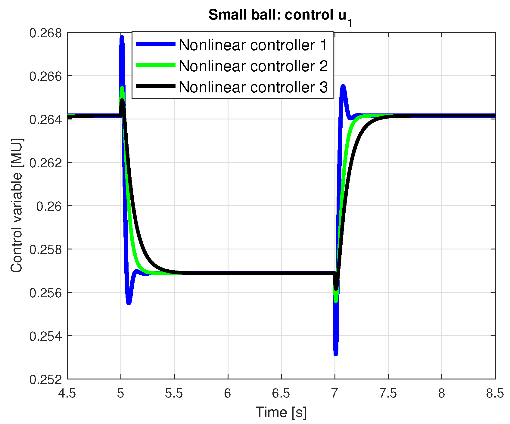
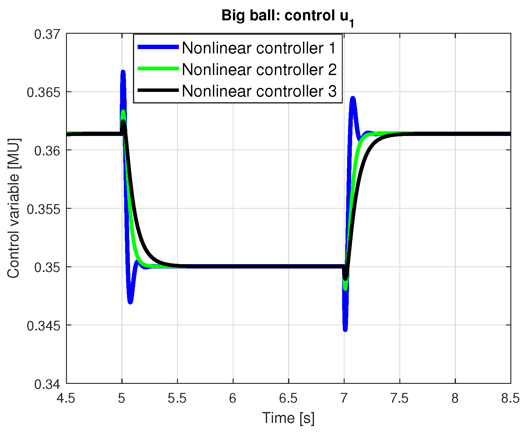
The resulting nonlinear control law (29) have been implemented in the magnetic levitation simulation model. Simulation results for step changes around the ball position $pos=0.01$ m for small and big ball cases are shown in Figure 11, Figure 12, Figure 13 and Figure 14. It should be noted, that step responses for ball position are with nonlinear control very similar for all three balls, therefore the responses for medium ball are omitted. Control variable differs in amplitude due to different ball masses, the shape of transient responses is again very close to each other for all three balls.

4.3. Comparison of Robust Pole-Placement and Nonlinear Controller for Magnetic Levitation

This section compares simulation results for robust pole-placement controller and a nonlinear controller, considering best designs in both cases. To test qualities of the compared controllers, in simulation experiment the required position is changed between 0.01 and 0.015 m, the latter provides upper limit for ball position feasible in simulation for all considered controllers. It can be assumed that the real system limit is even lower. The considered controllers are

-

nonlinear controller designed for continuous-time closed-loop poles

$P=[-500,-100,-50,-15]$, providing the best performance from tested nonlinear ones;

-

robust discrete-time pole-placement controller designed for AE region with design parameters: prescribed damping given by angle 70, $xe=0.7$, and stability degree $r=0.99$.

Simulation results for all three balls are shown in Figure 15, Figure 16, Figure 17, Figure 18, Figure 19 and Figure 20.

Presented comparison shows that the discrete-time pole-placement controller designed for AE region can compete with the continuous-time controller even for relatively big step change of ball position near the limit of feasible setpoints. In Figure 21 the closed-loop poles for both robust linear discrete-time and nonlinear continuous-time controllers are shown. The continuous-time poles are recalculated with sampling period $T_s$ = 0.001 s for all three designed controllers. Robust discrete-time poles correspond to three WPs, therefore we can see 3 times more poles than the system dimension. In the discrete-time case, some of poles are complex conjugated. On the other hand, the dominant poles depicted in detail are close to each other both for robust linear and nonlinear cases. This also confirms the competitiveness of the robust discrete-time pole-placement controller designed for AE region.

Finally, we can summarize the advantages and disadvantages of studied control approaches for nonlinear ML system.

Robust discrete-time pole-placement controller

Advantages:

• pole region instead of exact pole position is prescribed, which can be less demanding both on determining it and on corresponding control effort;
• control design is realized as off line solution of LMIs which is computationally efficient;
• the resulting control law is simple-implemented as state feedback gains;
• robust pole-placement is flexible and various uncertainties as different ball position or ball mass can be easily incorporated into the uncertain model and corresponding controller design.

Disadvantages:

• The main disadvantage of robust pole-placement controller is, that it is designed as a controller with constant gains for the whole uncertainty domain, which limits its use; this can be illustrated in responses in Figure 15, Figure 17 and Figure 19, where the response is nearly the same for nonlinear controller, while for a robust linear one there are significant differences; for the big ball the robust linear controller provides an oscillating response.

Nonlinear continuous-time controller

Advantages:

• The nonlinear control law follows the changing system parameters, for example, ball mass appears explicitly in control law (29). Therefore, the responses are very close to each other for different ball masses. This feature can be advantageous also for other parameter changes.

Disadvantages:

• in feedback linearization design, the exact closed-loop poles are to be prescribed, which are not easy to determine appropriately, since the closed-loop system proves as rather sensitive to pole-position, for example there is a problem when the complex poles are prescribed;
• control law is rather complicated and its implementation is more demanding, since several nonlinear feedback dependent formulas must be computed on-line;
• for simplification of the control law, the appropriate approximations of nonlinear terms should be used which must be found by optimization.

5. Conclusions

The main aim of this paper is in comparison of two principally different approaches to a nonlinear unstable Magnetic levitation system control. The nonlinear continuous-time control based on feedback linearization is compared with a robust pole-placement discrete-time controller for a linearized uncertain polytopic model. The main contribution of the paper can be summarized as: simplified development of nonlinear control law with novel approximation of nonlinear terms; developed robust pole-placement controller for different levitating balls and mainly a comparison and evaluation of the obtained results for both cases. The efficiency of the recently developed robust pole-placement linear controller was shown as well as the advantages and disadvantages of both approaches applied to Magnetic levitation.