Design of an IMCPID Optimized Neural Network for Stepless Flow Control of Reciprocating Mechinery

Abstract

It is usually difficult to design a controller for a nonlinear multiple-input and multiple-output (MIMO) system. The methodological approach taken in this study is a mixed methodology based on a PID-type internal model control (IMC) method and neural network (NN) optimization algorithm. The NN controller is designed for adjusting the sole parameter in IMCPID and compensating the characteristic changes and non-linearity in stepless flow control. In this study, a simulation of a nonlinear MIMO system with strong coupling is carried out. The simulation results indicate that the proposed control method has a better performance in settle time, overshoot, robustness and set-point tracking accuracy compared with other considered methods.

1. Introduction

Reciprocating compressors are widely used in some industrial fields such as petroleum, chemical, natural gas transportation and so on. It is the main power-consuming equipment in industrial factories and it is usually run at factory setting. However, in some conditions, the outlet flow of compressors needs to be regulated with the real-time demand of the downstream production process. Therefore, it is necessary and meaningful to control the outlet flow of compressors. Many approaches have been proposed, and the by-pass regulation is the simplest and most reliable method [1]. However, this method will cause a huge waste of electricity because the reflux gas will be sent back to the inlet of the compressor to be compressed again. In comparison with the by-pass regulation, the stepless flow control method has a better energy-saving performance because excess gas will be expelled from the compression cylinder prior to the compression process. Thus, this part of the gas will not be compressed, and some power consumption can be reduced. After equipping with the stepless flow control system, the effective power of the compressor will be greatly improved, and a lot of electricity will be saved. The stepless flow control system for the reciprocating compressor should meet the following requirements [2,3]:

• The control system should be capable of continuous stepless flow regulation within 0~100% working load.
• The control system should require low investment and low energy consumption.
• The control system should be reliable, safe and convenient to operate.
• The control system should have a wide range of applications.

From the point of view of control science, the stepless flow control system has multiple controlled variables and multiple manipulated variables [4]. The inlet flow of each stage is the manipulated variable, and the outlet gas pressure of each stage is the controlled variable. Thus, this is a multiple-input and multiple-output (MIMO) system. The primary feature of MIMO system is the strong coupling, where each manipulated variable can affect the other controlled variables. It is harder to design the controller than the single-input and single-output (SISO) system due to the interaction process between controlled variables and manipulated variables. Thus, one of the main control objectives for a MIMO system is reducing the coupling. Many approaches have been proposed to solve this control problem in state space and transfer function matrix representations. Some frequency-based frameworks have been researched in this study including the relative gain array (RGA) measure, feed-forward decoupling method, IMCPID and neural network [5].

The Proportional Integral Derivative (PID) control has been widely used in the industrial fields due to its simple structure and stable characteristics. However, for some dynamic processes such as time-delay, nonlinearity and coupling, the PID controller does not always represent high efficiency. In the past decades, the question of how to find simpler PID tuning methods has caught a mass of interest [6]. In both academic research and engineering applications, many PID-type controller designs have been developed, such as the famous Ziegler-Nichols (ZN) tuning rules [7], the well-know H₂/H_∞ robust optimal design method [8], the internal model control principle [9] and neural network PID [10]. In the above methods, IMC is considered as the simplest tuning rule of PID controller. This because all the three controller parameters of PID can be obtained from the only user-defined tuning parameter of IMC called λ (λ > 0). It is easy to control the linear or nonlinear, time-delay and coupling systems for the IMC scheme due to its simple and robust performance characteristics [11].

Many studies have been conducted to obtain PID tuning methods using IMC schemes which are achieved by complex mathematical manipulations or require a filter algorithm. For the stable linear and separable nonlinear system, an IMC-based PID (IMCPID) tuning scheme employing first-order in place of second or higher-order filter is presented [12]. Some heuristic methods have also been developed to get PID parameters [13,14,15]. A IMCPID controller has been slightly modified in [16] to demonstrate the importance of mid-frequency and high-frequency robustness for tuning parameters. As some processes having model uncertainty, [17] proposed an IMC tuning method based on gain margin and maximum peak criterion.

In order to eliminate the effects of uncertainty of system parameters, some adaptive control methods have been used in industrial processes [18,19]. The model-reference adaptive control and self-tuning regulator control can effectively solve the disturbance problem in linear system [20]. The method in [21] combines IMC and adaptive PSD control. The result of applying it to the main steam temperature system shows that the method is effective. However, the parametric uncertainties and external disturbances of nonlinear systems are more sophisticated than those of linear systems. To solve this problem, some intelligent techniques [11] have been applied to adaptive controller, including neural network and fuzzy logic control, etc. Paper [22] presents an IMCPID control method to modified the weight of the set-point online with fuzzy logic, which can improve the set-point tracking performance and robustness of the system. In paper [23], the technique of the self-tuning neural network PID control for the stabilizer fin to reduce ship rolling motion is successfully developed. Because the neural network can approximate any continuous function, the adaptive controller based on neural networks has excellent online estimation characteristics [22].

In this paper, a neural network based on IMCPID control strategy is proposed to improve the performance of the stepless flow controller. A feedforward decoupling method is designed which can eliminate the coupling and transform the multiloop system into several independent single-input and single-output loops [24]. In the feedback loop, an adaptive IMCPID control method is proposed which uses the system error as the input signal of the neural network and regulates the IMCPID parameter λ by its self-learning in real time [23]. The main purpose of this paper is to solve the problem of PID parameter setting in the actual industrial field operation process, which is usually a complex job. Therefore, we proposed a more concise neural network combined with an IMCPID control method, which reduces the number of system parameters and the difficulty of parameter setting. Some researchers found out that after applying neural networks to these nonlinear systems, not only will the parameter tuning process become simpler, but also the control performance will present more excellently [25]. PID neural network will automatically adjust the control parameters due to its self-organizing, self-learning and self-adaptation characteristics [26]. The simulation experiments show that the IMCPID controller based on neural network for a stepless flow control system has better performances in set-point tracking, stability and robustness than those of the other considered controllers.

The rest of this paper is organized as follows. Section 2 gives the mathematical model for a stepless flow control system of a reciprocating compressor. In Section 3, The IMCPID-based neural network (IMCPIDNN) control scheme is presented. The simulation results of a multivariable nonlinear control system are compared and discussed in Section 4. Finally, the conclusion and some open problems are given in Section 5.

2. Problem Formulation

The stepless flow control system for a two-cylinder type reciprocating compressor [27] is shown in Figure 1, where $r$ denotes the gas to be compressed and $y$ denotes the compressed gas. In standard operating conditions, the gas satisfies the following ideal gas assumptions:

$$P=\frac{\rho RT}{M},$$

(1)

$$\dot{m}=\frac{d}{dt}(\rho V),$$

(2)

$${\dot{m}}_{in}-{\dot{\mathit{m}}}_{out}=\rho \dot{V}+\dot{\rho }V,$$

(3)

where $\mathit{P}$ is gas pressure, $\rho$ is gas density, $\mathit{R}$ is gas constant, $\mathit{T}$ is gas temperature, $\mathit{M}$ is gas molar mass, $\mathit{m}$ is derivative of gas mass, $\mathit{V}$ is gas volume, ${\dot{m}}_{in}$ is derivative of the gas mass flowing into the cylinder, ${\dot{m}}_{out}$ is derivative of the gas mass flowing out of the cylinder and $\dot{V}$ and $\dot{\rho }$ are derivatives of the gas volume and gas density, respectively. Usually, the gas volume is invariable in the buffer tank, so $V=0$.

Combining Equations (1)–(3), the dynamic pressure change of the cylinder can be described as:

$$\dot{P}=\frac{RT}{V}({\varphi }_{in}{\dot{\mathit{m}}}_{in}-{\varphi }_{out}{\dot{\mathit{m}}}_{out}),$$

(4)

where ${\varphi }_{in}$ and ${\varphi }_{out}$ are process coefficients of the inlet gas or outlet gas, which are ranging from 0 to 1 depending on the gas process characteristic.

According to the mathematical model for reciprocating compressors introduced in paper [28], the gas mass flowing into the first stage cylinder and the second stage cylinder during the compressing process can be given as Equations (5) and (6), respectively.

$${\dot{\mathit{m}}}_{in1}=\frac{P_{s1}}{R_m}\frac{M}{T_{s1}}\frac{1}{T}{V}_{h1}{\omega }_{p1}{w}_{t1}{w}_{l1}[1+{\sigma }_1-{\sigma }_1{(\frac{P_1}{P_{s1}})}^{\frac{1}{m_1}}]{\theta }_1,$$

(5)

$${\dot{\mathit{m}}}_{in2}=\frac{P_1}{R_m}\frac{M}{T_{s2}}\frac{1}{T}{V}_{h2}{\omega }_{p2}{w}_{t2}{w}_{l2}[1+{\sigma }_2-{\sigma }_2{(\frac{P_2}{P_1})}^{\frac{1}{m2}}]{\theta }_2,$$

(6)

where ${\mathit{P}}_{\mathit{s}}$ is pressure of inlet gas, ${\mathit{R}}_{\mathit{m}}$ is gas constant, ${\mathit{T}}_{\mathit{s}}$ is temperature of inlet gas, $\mathit{T}$ is temperature of buffer tank, ${\mathit{V}}_{\mathit{h}}$ is volume of cylinder stroke volume, ${\mathsf{\omega }}_{\mathit{p}}$ is pressure coefficient, ${\mathsf{\omega }}_{\mathit{t}}$ is temperature coefficient, ${\mathsf{\omega }}_{\mathit{l}}$ is leakage coefficient, $\mathsf{\sigma }$ is volume coefficient, $\mathit{P}$ is pressure of buffer tank, $\mathit{m}$ is gas mass and $\mathsf{\theta }$ is working load. The subscript $\mathit{i} (\mathit{i}=1, 2)$ indicates the cylinder number of the compressor.

The gas compressed by the first stage cylinder will be sent into the second stage cylinder. Then, we can obtain the relationship between the outlet mass of the first-stage cylinder and the inlet mass of the second-stage cylinder.

$${\dot{\mathit{m}}}_{out1}={\dot{m}}_{in2}.$$

(7)

Considering the dynamic principle of the exhaust valve, the equation of the outlet mass of the second-stage cylinder can be expressed as

$${\dot{m}}_{out2}=C_f{A}_0{C}_1\frac{P_2}{\sqrt{T_2}}.$$

(8)

Combing Equations (4)–(8), the dynamic change of cylinder pressure can be presented as:

$${\dot{P}}_1=\frac{R{T}_1}{V_1}\left\{\begin{array}{l}{\sigma }_{in1}\frac{P_{s1}}{R_m}\frac{M}{T_{s1}}\frac{1}{T}{V}_{h1}{\omega }_{p1}{w}_{t1}{w}_{l1}[1+{\sigma }_1-{\sigma }_1{(\frac{P_1}{P_{s1}})}^{\frac{1}{m_1}}]{\theta }_1\\ -{\sigma }_{out1}\frac{P_1}{R_m}\frac{M}{T_{s2}}\frac{1}{T}{V}_{h2}{\omega }_{p2}{w}_{t2}{w}_{l2}[1+{\sigma }_2-{\sigma }_2{(\frac{P_2}{P_1})}^{\frac{1}{m2}}]{\theta }_2\end{array}\right\},$$

(9)

$${\dot{P}}_2=\frac{R{T}_2}{V_2}\left\{\begin{array}{l}{\sigma }_{in2}\frac{P_1}{R_m}\frac{M}{T_{s2}}\frac{1}{T}{V}_{h2}{\omega }_{p2}{w}_{t2}{w}_{l2}[1+{\sigma }_2-{\sigma }_2{(\frac{P_2}{P_1})}^{\frac{1}{m2}}]{\theta }_2\\ -{\varphi }_{out2}{C}_f{A}_0{C}_1\frac{P_2}{\sqrt{T_2}}\end{array}\right\}.$$

(10)

The operation parameters of a two-cylinder reciprocating compressor with a stepless flow control system are listed in

Table 1. Operation parameters of a two-cylinder reciprocating compressor.

Item	Value	Unit
Rated speed	300	r/min
Suction pressure	0.1	MPa
Number of suction valves	8
Number of exhaust valves	8
Number of cylinders	2
Buffer tank volume of first cylinder exit	0.3	m3
Buffer tank volume of second cylinder exit	1.5	m3
Quantity of flow	1.2	m3/h
Stroke volume	0.0086	m3
Pressure coefficient	0.95
Temperature coefficient	0.9
Leakage coefficient	0.125
Volume coefficient	1.25
Expansion index	0.25
Cross-sectional area of export valve	0.007885	m3
Intake temperature of first cylinder	313	K
Exhaust temperature of first cylinder	343	K
Exhaust temperature of second cylinder	293	K

.

Substituting the operation parameter values in Table 1 into Equations (9) and (10), the relationship between the outlet pressure and working load can be written as Equation (11), where ${\mathit{y}}_1$ and ${\mathit{y}}_2$ are outlet pressure, ${\mathit{u}}_1$ and ${\mathit{u}}_2$ are working load of each cylinder, respectively, and $\mathsf{\xi }$ is the opening of outlet:

$$\left\{\begin{array}{l}\frac{d{y}_1}{dt}=29422u_1+5547.82+0.082y_1{u}_2+0.0142y_2\\ \frac{d{y}_2}{dt}=0.0106y_1+0.057y_1{u}_2-0.00562y_2-0.072y_2\sqrt{323}\xi \end{array}\right..$$

(11)

3. Controller Design

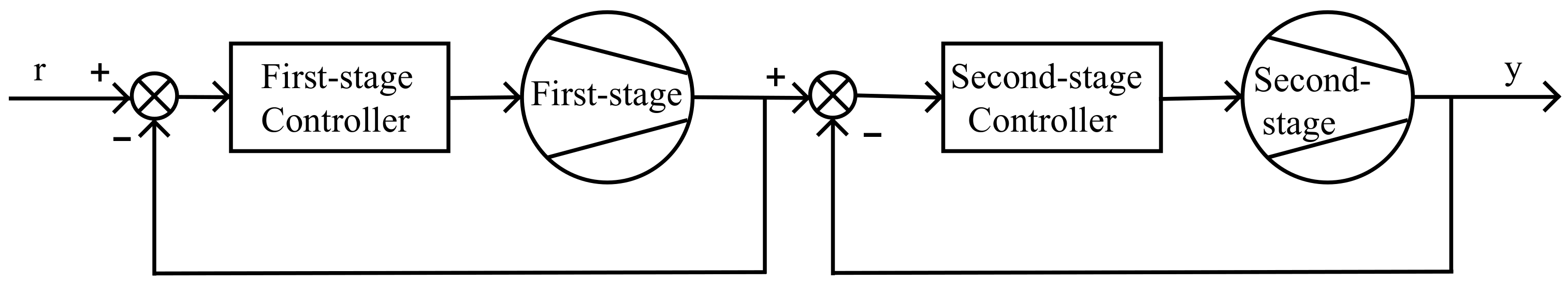
In this section, the set-point tracking and decoupling control scheme will be proposed. The basic structure of the IMCPIDNN control system is shown in Figure 2. The design process of the IMCPIDNN controller mainly consists of four parts: relative gain array, feed-forward decoupling, IMC controller based on standard PID and IMCPIDNN controller design. In the whole control system, $r(k)$ is set-point value, $e(k)$ is error of subtracting the output value from the set-point value, $y(k)$ is output value, $u(k)$ is control signal, $\lambda (k)$ is the only IMCPID controller parameter to be adjusted and $d$ is external disturbance. The whole control algorithm is established based on the adaptive IMCPID controller and neural network algorithm, which is presented in Algorithm 1.

Algorithm 1 IMCPIDNN algorithm for MIMO nonlinear system.

Step 1: Initialize the weights of IMCPIDNN.

Step 2: Input the set-point value of controlled system into the controller.

Step 3: Regulate the compressor flow by IMCPIDNN controller.

Step 4: Calculate error and evaluation function.

Step 5: Adjust the weights of IMCPIDNN controller by back propagation algorithm.

Step 6: Repeat steps 3 to 5.

Step 7: Stop the algorithm until the error is small enough. If not, return to Step 3.

3.1. Relative Gain Array (RGA)

As we can see in Equation (11), there are two controlled variables and two manipulated variables in the presented control process. There are two ways to pair control variables with operation variables and they are ${\mathit{u}}_1{-\mathit{y}}_1{/\mathit{u}}_2{-\mathit{y}}_2$ and ${\mathit{u}}_1{-\mathit{y}}_2{/\mathit{u}}_2{-\mathit{y}}_1$, respectively. To find which configuration has a better performance in terms of resisting the system coupling, the RGA method is proposed. For the system ${\mathit{G}}_{\mathit{m}}\left(\mathit{s}\right)$ with n inputs and m outputs, its RGA can be calculated by:

The RGA method is proposed. For the system ${\mathit{G}}_{\mathit{m}}\left(\mathit{s}\right)$ with n inputs and m outputs, its RGA can be calculated by:

$$\beta (s)=[{\beta }_{ij}(s)]=G_m(s)\cdot *{[G_m{(s)}^{-1}]}^T{}_{j=1,2,...,n}^{i=1,2,...,m},$$

(12)

where * is the multiplication of Hadamard.

Considering that the sum of each row and each column is 1, the RGA for a two-input and two-output system satisfies the following equation:

$$\left\{\begin{array}{l}{\beta }_{11}(s)={\beta }_{22}(s)\\ {\beta }_{12}(s)={\beta }_{21}(s)\\ {\beta }_{11}(s)+{\beta }_{12}(s)=1\end{array}\right.,$$

(13)

where ${\mathsf{\beta }}_{11}\left(\mathit{s}\right)$ and ${\mathsf{\beta }}_{22}\left(\mathit{s}\right)$ are the relative gains of main channel and ${\mathsf{\beta }}_{12}\left(\mathit{s}\right)$ and ${\mathsf{\beta }}_{21}\left(\mathit{s}\right)$ are the relative gains of coupled channel.

Therefore, the whole RGA matrix can be calculated from ${\mathsf{\lambda }}_{11}\left(\mathit{s}\right)$. In the RGA method, the value of $\mathsf{\beta }\left(\mathit{s}\right)$ describes the coupling degree within the system. If is $\mathsf{\beta }\left(\mathit{s}\right)$ close to 1, every loop can be considered to run independently. If it is close to 0, the coupling is serious. Negative $\mathsf{\beta }\left(\mathit{s}\right)$ must be avoided because it results in instability. Therefore, we should choose the $\mathsf{\beta }\left(\mathit{s}\right)$ which is positive and close to 1 to be the best configuration.

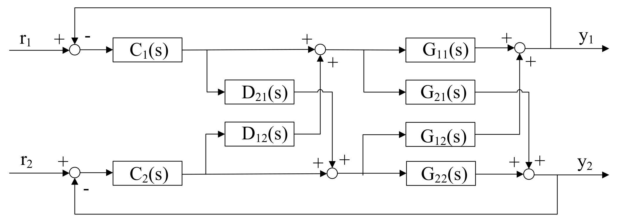
3.2. Feed-Forward Decoupling

The undesirable dynamic coupling within the system will affect the stability and control performance of the stepless control system [29]. This paper introduces a simple and efficient feed-forward decoupling method to eliminate the coupling, and the block diagram for a two-input and two-output system is shown in Figure 3 [24].

Here, ${\mathit{r}}_{\mathit{i}}$ is the set-point value, ${\mathit{y}}_{\mathit{j}}$ is the output value, ${\mathit{C}}_{\mathit{i}}\left(\mathit{s}\right)$ is the proposed controller, ${\mathit{G}}_{\mathrm{ij}}\left(\mathit{s}\right)$ is the process plant and $D_{\mathrm{ij}}\left(s\right)$ is the decoupler.

Supposing the system is decoupled completely, the transfer function matrix will turn into a diagonal matrix. $D_{21}\left(s\right)$ and $D_{12}\left(s\right)$ satisfy the following relationship:

$$\left\{\begin{array}{l}{u}_1{G}_{21}(s)+u_1{D}_{21}(s)G_{22}(s)=0\\ u_2{G}_{12}(s)+u_2{D}_{12}(s)G_{11}(s)=0\end{array}\right..$$

(14)

Then, we can obtain $D_{21}\left(s\right)$ and $D_{12}\left(s\right)$ as:

$$\left\{\begin{array}{l}{D}_{21}(s)=-\frac{G_{21}(s)}{G_{22}(s)}\\ D_{12}(s)=-\frac{G_{12}(s)}{G_{11}(s)}\end{array}\right..$$

(15)

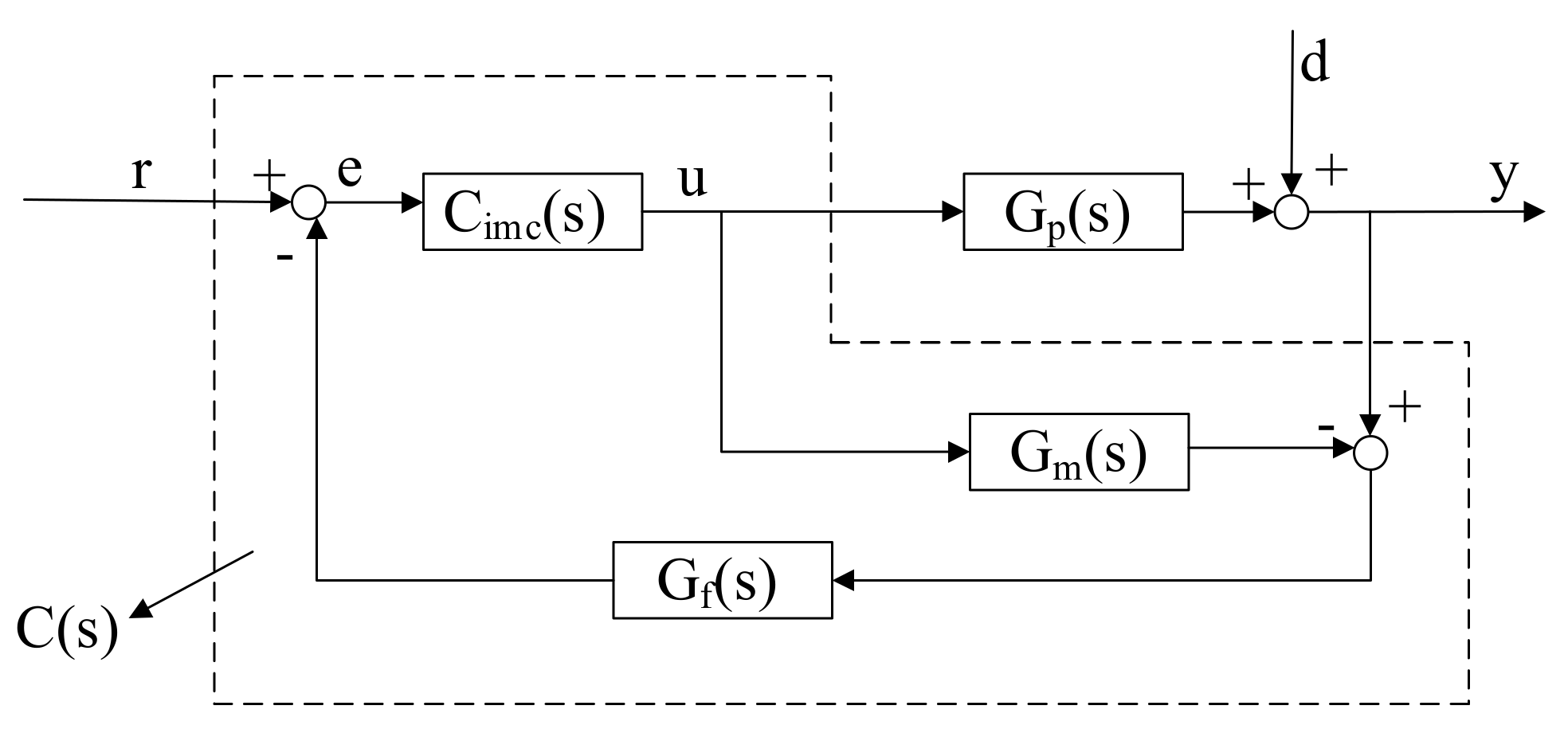
3.3. IMC Controller Design Based on Standard PID

In this part, an improved IMC control based on standard PID controller and classical feedback structures is proposed. The Standard IMC structure is presented in Figure 4, where $G_p\left(s\right)$ is the process, $G_m\left(s\right)$ is the process model, $G_f\left(s\right)$ is the filter, $C_{\mathrm{imc}}\left(s\right)$ is IMC controller and $C\left(s\right)$ is the IMC controller with feedback structure.

The closed-loop transfer function obtained from Figure 4 is:

$$y=\frac{C_{imc}(s)G_p(s)}{1+C_{imc}(s)[G_p(s)-G_m(s)]}r+\frac{1-C_{imc}(s)G_m(s)}{1+C_{imc}(s)[G_p(s)-G_m(s)]}d.$$

(16)

If the process model is completely accurate, it is $G_m{\left(s\right)=G}_p\left(s\right)$, and the external disturbances $d=0$. Then, Equation (16) can be written as:

$$y=C_{imc}(s)G_p(s)r.$$

(17)

From Equation (17), we find an interesting property: the closed-loop transfer function can be considered as an open-loop system only related to ${\mathit{C}}_{\mathrm{imc}}\left(\mathit{s}\right)$. The designing process of the IMC controller can be regarded as the product of the inverted process and the closed-loop transfer function.

The design process of the IMCPID controller includes three steps which are shown in Algorithm 2.

Algorithm 2 The design process of the IMCPID controller.

Step 1: Factorize ${\mathit{G}}_{\mathit{m}}\left(\mathit{s}\right)$

$$G_m(s)=G_m^{-}(s)G_m^{+}(s),$$ (18)

where ${\mathit{G}}_{\mathit{m}}^{-}\left(\mathit{s}\right)$ contains the minimum phase part of the model and ${\mathit{G}}_{\mathit{m}}^{+}\left(\mathit{s}\right)$ contains all the right half plane zeros and the time delays of ${\mathit{G}}_{\mathit{m}}\left(\mathit{s}\right)$. $\left|{\mathit{G}}_{\mathit{m}}^{+}\left(0\right)\right| = 1$.

Step 2: Design ${\mathit{C}}_{\mathrm{imc}}\left(\mathit{s}\right)$ and ${\mathit{G}}_{\mathit{f}}\left(\mathit{s}\right)$

$$\left\{\begin{array}{l}{C}_{imc}(s)=\frac{1}{G_m^{-}(s)}{G}_f(s)\\ G_f(s)=\frac{1}{{(\lambda s+1)}^n}\end{array}\right.$$ (19)

where ${\mathit{G}}_{\mathit{f}}\left(\mathit{s}\right)$ is the filter which provides good performance for set-point tracking and disturbance suppression, $\mathsf{\beta }$ is the time constant of ${\mathit{G}}_{\mathit{f}}\left(\mathit{s}\right)$ and the only tuning parameter of the IMC controller that affects the closed-loop response and stability and $\mathit{n}$ is the filter order decided by ${\mathit{G}}_{\mathit{m}}^{-}\left(\mathit{s}\right)$.

Step 3: Calculate the IMCPID controller $\mathit{C}\left(\mathit{s}\right)$ and turn it into the PID-type

$$\begin{array}{ll}C(s)& =\frac{C_{imc}(s)}{1-G_m(s)C_{imc}(s)}\\ & =\frac{G_f(s)}{G_m^{-}(s)-G_f(s)G_m(s)}\\ & =K_p(1+\frac{1}{T_i}s+T_d(s))\end{array}$$ (20)

where ${\mathit{K}}_{\mathit{p}}$, ${\mathit{T}}_{\mathit{I}}$ and ${\mathit{T}}_{\mathit{d}}$ are proportional gain, integral time and derivative time, respectively.

Most industrial processes can be represented by a first-order model plus time-delay system as shown below:

$$G_m(s)=\frac{k}{ts+1}{e}^{-\tau s},$$

(21)

where $k$, $t$ and $\tau$ are open-loop gain, time constant and delay time, respectively.

Considering that the delay time $e^{-\tau s}$ is difficult to implement physically, we could replace it with first the order Pade approximation, that is, $e^{-\tau s}=1-\tau s$. Then, $G_m\left(s\right)$ can be factorized as:

$$G_m(s)\approx \frac{k}{ts+1}\frac{1-\frac{\tau }{2}s}{1+\frac{\tau }{2}s}.$$

(22)

${\mathit{G}}_{\mathit{m}}^{+}\left(\mathit{s}\right)$ and ${\mathit{G}}_{\mathit{m}}^{+}\left(\mathit{s}\right)$ can be obtained as:

$$G_m^{+}(s)=1-\frac{\tau }{2}s,$$

(23)

$$G_m^{-}(s)=\frac{k}{(ts+1)(1+\frac{\tau }{2}s)}.$$

(24)

The filter order $\mathit{n}$ should be consistent with the system order, that is, $\mathit{n}=1$. Substituting Equations (19), (22) and (24) into Equation (20), the PID-type IMCPID controller can be written as:

$$C(s)=\frac{2t+\tau }{k(2\lambda +\tau )}(1+\frac{2}{\tau +2t}\frac{1}{s}+\frac{t\tau }{\tau +2t}s).$$

(25)

Then, the PID parameters can be presented by the following equation:

$$\left\{\begin{array}{l}{K}_p=\frac{2t+\tau }{k(2\lambda +\tau )}\\ K_i=\frac{2}{\tau +2t}\\ K_d=\frac{t\tau }{\tau +2t}\end{array}\right.,$$

(26)

where ${\mathit{K}}_{\mathit{p}}$ is proportional gain, ${\mathit{K}}_{\mathit{a}}$ is integral gain and ${\mathit{K}}_{\mathit{d}}$ is differential gain, respectively.

3.4. IMCPIDNN Controller Design

In order to compensate the nonlinearity of the stepless flow control system, the neural network algorithm based on the IMCPID control scheme is proposed [30]. The block diagram of a MIMO system with a backpropagation (BP) neural network structure is as shown in Figure 5.

Here, $\mathit{r}$ and $\mathit{y}$ are set-point value and output value, respectively. ${\mathit{W}}_{\mathrm{if}}$ is the network weight between the ${\mathit{j}}_{\mathrm{th}}$ node of the input layer and the ${\mathit{i}}_{\mathrm{th}}$ node of the hidden layer and ${\mathit{W}}_{\mathit{i}}$ is the network weight between the ${\mathit{i}}_{\mathrm{th}}$ node of the hidden layer and the output layer node.

From Equation (26), the discrete PID gains can be written as:

$$\left\{\begin{array}{l}{K}_p(k)=\frac{2t+\tau }{k(2\lambda (k)\gamma +\tau )}\\ K_i(k)=\frac{2}{k(2\lambda (k)\gamma +\tau )}\\ K_d(k)=\frac{t\tau }{k(2\lambda (k)\gamma +\tau )}\end{array}\right.,$$

(27)

where $\gamma$ is the tuning coefficient to determine the flexibility of the control process.

Then, according to the incremental PID principle [31], the output of IMCPID controller can be written as:

$$\begin{array}{l}u(k)=u(k-1)+[K_P(k)+K_I(k)+K_D(k)]e(k)\\ -[K_P(k)+2K_D(k)]e(k-1)+K_D(k)e(k-2)\end{array}$$

(28)

In this article, a three-layer BP neural network is proposed as show in Figure 5. There are five input nodes, six hidden nodes and one output node in the neural network structure.

The input of the neural network is defined as:

$$I_j(k)=[r(k),y(k),e(k-1),u(k-1)](j=1,2,3,4).$$

(29)

The input of the hidden layer is defined as:

$$ne{t}_i(k)={\displaystyle \sum _{j=0}^4{W}_{ij}\cdot I_j(k)(i=1,2,...,6)}.$$

(30)

The output of the hidden layer is defined as:

$$O_i(k)=f[ne{t}_i(k)],$$

(31)

where $\mathit{f}\left(\mathit{x}\right)$ is the sigmoid function:

$$f(x)=\frac{1}{1+e^{-x}}.$$

(32)

The input of the output layer is defined as:

$$net(k)={\displaystyle \sum _{j=0}^6{W}_i\cdot O_i}.$$

(33)

The output of the output layer is defined as:

$$\lambda (k)=g[net(k)],$$

(34)

where $\mathit{g}\left(\mathit{x}\right)$ is a non-negative sigmoid function to ensure the outputs to be positive as shown below:

$$g(x)=\frac{e^x}{1+e^{-x}}.$$

(35)

The central ideal of the learning algorithm for the IMCPIDNN is to obtain a gradient vector recursively. In this study, we define energy function as:

$$J(k)=\frac{1}{2}{[r(k)-y(k)]}^2.$$

(36)

In order to get the minimum $J(k)$, the iterative algorithm of $\Delta w_i(k)$ can be calculated as the following equation according to the gradient descent method:

$$\begin{array}{ll}\Delta w_i(k)& =w_i(k)-w_i(k-1)\\ & =\alpha \Delta w_i(k-1)+\eta \frac{\partial J(k)}{\partial w_i(k)}\end{array}$$

(37)

where $\mathsf{\eta }$ is the learning rate, and $\mathsf{\eta } > 0$; $\alpha$ is the inertial coefficient, and $\frac{\partial J\left(k\right)}{\partial W_i\left(k\right)}$ can be written as:

$$\frac{\partial J(k)}{\partial w_i(k)}=\frac{\partial J(k)}{\partial y(k)}\frac{\partial y(k)}{\partial u(k)}\frac{\partial u(k)}{\partial \lambda (k)}\frac{\partial \lambda (k)}{\partial net(k)}\frac{\partial net(k)}{\partial w_i(k)}.$$

(38)

From Equation (37), we can obtain:

$$\frac{\partial J(k)}{\partial y(k)}=-e(k).$$

(39)

Considering that $\frac{\partial \mathit{y}\left(\mathit{k}\right)}{\partial \mathit{u}\left(\mathit{k}\right)}$ cannot be written [32], we use the sign function to approximate it.

Combining Equations (27) and (28), we can obtain $\frac{\partial \mathit{u}\left(\mathit{k}\right)}{\partial \mathsf{\lambda }\left(\mathit{k}\right)}$ as below:

$$\begin{array}{ll}\frac{\partial u(k)}{\partial \lambda (k)}=& -[{\overline{K}}_P(k)+{\overline{K}}_I(k)+{\overline{K}}_D(k)]e(k)\\ & +[{\overline{K}}_P(k)+2{\overline{K}}_D(k)]e(k-1)-{\overline{K}}_D(k)e(k-2)\end{array}$$

(40)

where ${\overline{K}}_P(k)$, ${\overline{K}}_I(k)$ and ${\overline{K}}_D(k)$ are the discrete style of $K_P(k)$, $K_I(k)$ and $K_D(k)$, respectively.

$$\left\{\begin{array}{l}{\overline{K}}_P(k)=\frac{2\gamma (2t+\tau )}{k{[2\lambda (k)\gamma +\tau ]}^2}\\ {\overline{K}}_I(k)=\frac{2\gamma }{k{[2\lambda (k)\gamma +\tau ]}^2}\\ {\overline{K}}_D(k)=\frac{2t\tau }{k{[2\lambda (k)\gamma +\tau ]}^2}\end{array}\right.,$$

(41)

From Equations (33) and (34), we can get $\frac{\partial \mathsf{\lambda }\left(\mathit{k}\right)}{\partial \mathrm{net}\left(\mathit{k}\right)}$ and $\frac{\partial \mathrm{net}\left(\mathit{k}\right)}{\partial {\mathit{W}}_{\mathit{i}}\left(\mathit{k}\right)}$ as:

$$\frac{\partial \lambda (k)}{\partial net(k)}=g[net(k)]=\lambda (k)[1-\lambda (k)],$$

(42)

$$\frac{\partial net(k)}{\partial w_i(k)}=h_j(k).$$

(43)

According to Equations (37)–(43), the output layer weight change $\Delta w_i(k)$ can be written as:

$$\Delta w_i(k)=\alpha \Delta w_i(k-1)+\eta {\delta }^{(1)}{h}_j(k-1),$$

(44)

where

$$\begin{array}{ll}{\delta }^{(1)}=& e(k)\mathrm{sgn}[\frac{\partial y(k)}{\partial u(k)}][-({\overline{K}}_P(k)+{\overline{K}}_I(k)+{\overline{K}}_D(k))e(k)\\ & +[{\overline{K}}_P(k)+2{\overline{K}}_D(k)]e(k-1)-{\overline{K}}_D(k)e(k-2)]\lambda (k)[1-\lambda (k)]\end{array}$$

(45)

The hidden layer weights $\Delta w_{ij}(k)$ can be obtained in the same way with the following equation:

$$\Delta w_{ij}(k)=\alpha \Delta w_{ij}(k-1)+\eta {\delta }^{(2)}{I}_j(k-1),$$

(46)

where

$${\delta }^{(2)}={\delta }^{(1)}{w}_{ij}(k-1)h_j(k-1)[1-h_j(k-1)].$$

(47)

Through the above derivation, we obtain the weight coefficient learning algorithm for the neural network, and only the parameter $\mathsf{\lambda }$ can be adjusted in real time according to the above derivation. The parameters of the IMCPIDNN controller are shown in

Table 2. Parameters of the IMCPIDNN controller.

Symbol	Parameter	Value
$\eta$	Learning coefficient	0.5
$\alpha$	Inertia coefficient	0.2
$l$	Number of input layer nodes	5
$j$	Number of hidden layer nodes	6
$i$	Number of output layer nodes	1

.

4. Algorithm Simulation and Results

In this section, some simulations are completed to illustrate the effect of the proposed IMCPIDNN controller in a stepless flow control system. The design and training process of IMCPIDNN and PID, IMCPID and FLSMC (feedback linearization sliding mode control) are done with the MATLAB/SIMULINK environment. Some possible external disturbances have also been taken into consideration during the simulation process. The simulation sampling time is set as 0.01s. The controller output threshold is set as $\left[0,1\right]$ to simulate the real action of the actuators. The learning rate $\eta$ and the inertial coefficient $\alpha$ are set as 0.5 and 0.1, respectively. In addition, the simulation results of the control effects are compared in terms of step responses, anti-interference and robustness, which shows the superior performance of the proposed IMCPIDNN controller in all aspects.

The industrial process presented in Section 2 is a two-input and two-output system whose open-loop transfer function can be described as:

$$G_m(s)=\left[\begin{array}{cc}\frac{244}{6s+1}{e}^{-s}& \frac{-394}{5s+1}{e}^{-3s}\\ \frac{254}{72s+1}{e}^{-s}& \frac{133}{13s+1}{e}^{-2s}\end{array}\right].$$

(48)

The RGA matrix is:

$$\beta (s)=\left[\begin{array}{cc}0.25& 0.75\\ 0.75& 0.25\end{array}\right].$$

(49)

According to the controller design method presented in Section 3, we know that the system coupling is serious, and the best paring configuration is $u_1/y_2$ and $u_2/y_1$. Thus, the process model $G_m\left(s\right)$ can be simplified as:

$$G_m(s)=\left[\begin{array}{cc}0& \frac{-394}{5s+1}{e}^{-3s}\\ \frac{254}{72s+1}{e}^{-s}& 0\end{array}\right].$$

(50)

The value of the filter parameter $n$ is selected as $n=1$ to meet the order of the model $G_m\left(s\right)$. The PID-IMC controller $G_c\left(s\right)$ can be obtained as the following equation according to the controller design method given in Equations (16)–(26):

$$G_m(s)=\left[\begin{array}{cc}0& -\frac{13}{394(2{\lambda }_1+3)}(1+\frac{2}{13}\frac{1}{s}+\frac{15}{13}s)\\ \frac{145}{254(2{\lambda }_2+1)}(1+\frac{2}{145}\frac{1}{s}+\frac{72}{145}s)& 0\end{array}\right].$$

(51)

4.1. Step Response Test and Validation

To demonstrate the characteristics of the proposed IMCPIDNN controller, step response tests are made for the reciprocating compressor numerical model. The PID controller, IMCPID controller and FLSMC controller are constructed to make comparisons under the same condition. The simulations are carried out with reference pressure profile under the simulated condition to verify the control performance of the proposed controller.

In order to evaluate the performance of the proposed controllers, we use the integral of absolute value error criterion (IAE), integral of time multiplied by the absolute value of error criterion (ITAE), integral of square error criterion (ISE) and integral of time multiplied by squared error criterion (ITSE) as the evaluation function [33]. Two-system step response performance indicators have also been applied and they are ${\mathit{t}}_{\mathit{s}}$ and ${\mathit{M}}_{\mathit{p}}$, where ${\mathit{t}}_{\mathit{s}}$ means the shortest time that reaches the step response steady-state value of 2% error and ${\mathit{M}}_{\mathit{p}}$ means the overshoot, respectively.

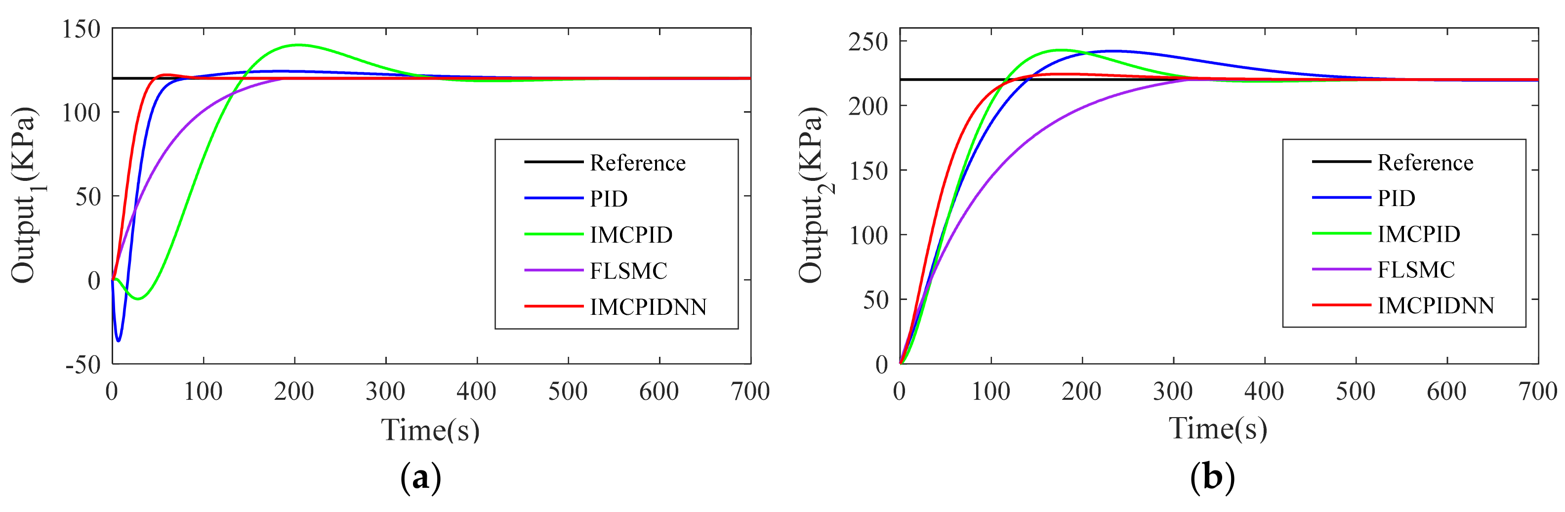
Figure 6 shows that the dynamic output of each loop meets the desired set point. The dynamic tracking performances obtained by PID, IMCPID, FLSMC and IMCPIDNN controllers for the two-input and two-output nonlinear system were compared. The process of starting the system from the shutdown state is imitated, where the set-points of the first output and the second output change from 0 kPa to 120 kPa and 220 kPa at moment t = 0 synchronously. Obviously, IMCPIDNN has the shortest settle time and the smallest overshoot, and it performs the best among the four algorithms while PID performs worst.

Table 3. Performance comparison of the four algorithms used for concurrent step responses.

Algorithm		${\mathbf{M}}_{\mathbf{p}} (\%)$	${\mathbf{t}}_{\mathbf{s}} \left(\mathbf{s}\right)$	IAE(×103)	ISE(×105)	ITAE(×105)	ITSE(×106)
Output1	PID	2.73	272.96	5.42	4.88	2.71	7.10
	IMCPID	9.73	319.01	11.53	9.24	8.65	38.42
	FLSMC	0	73.68	5.09	3.21	1.91	7.08
	IMCPIDNN	0	61.91	2.62	1.98	0.42	1.96
Output2	PID	7.63	435.42	16.70	18.96	15.99	65.07
	IMCPID	18.27	278.99	14.48	18.42	9.59	53.10
	FLSMC	0	102.54	16.47	19.43	10.70	73.88
	IMCPIDNN	0	82.83	10.60	14.05	4.01	31.14

presents the best control performance indices obtained by each controller. What stands out in the table is all the performance indices of the IMCPIDNN controller are optimal in the closed-loop step response. The value of the settle time ${\mathit{t}}_{\mathit{s}}$ of the step responses for the two loops are: 61.91 s and 146.78 s, respectively. They are smaller than those obtained by the other three algorithms. The IAE, ITAE, ISE and ITSE values obtained with the proposed algorithm for loop 1 are: 2.62, 1.98, 0.42 and 1.96, and for loop 2: 10.60, 14.05, 4.01 and 31.14. Compared with the PID controller, IMCPID controller and FLSMC controller, the proposed IMCPIDNN controller performs better in terms of set-point tracking.

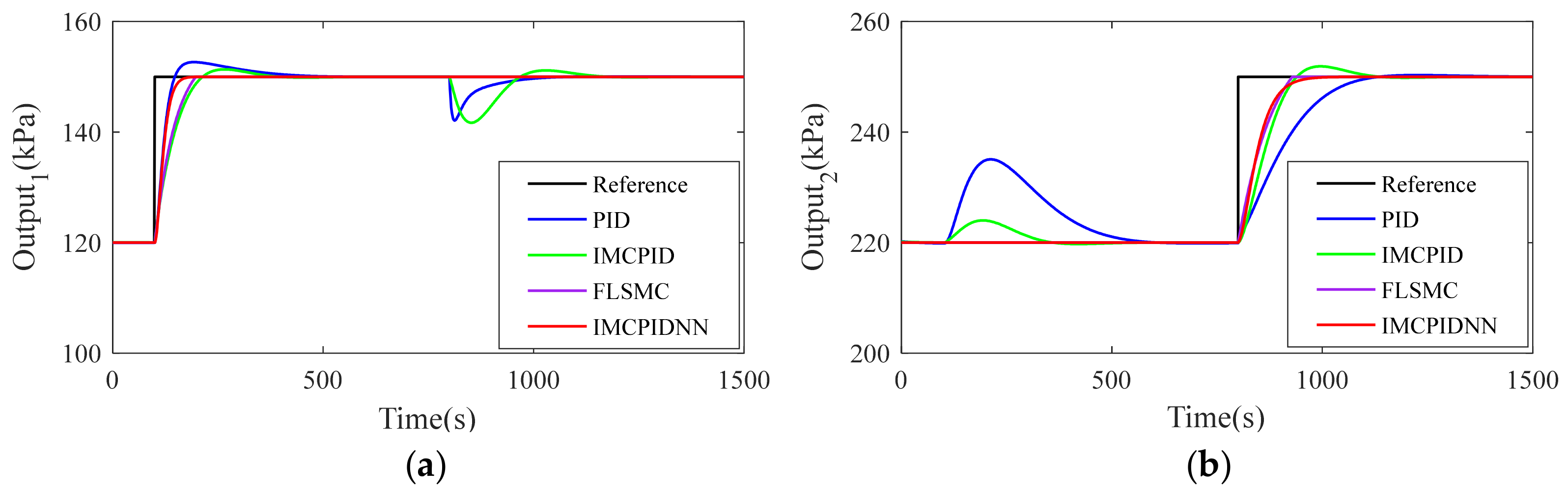
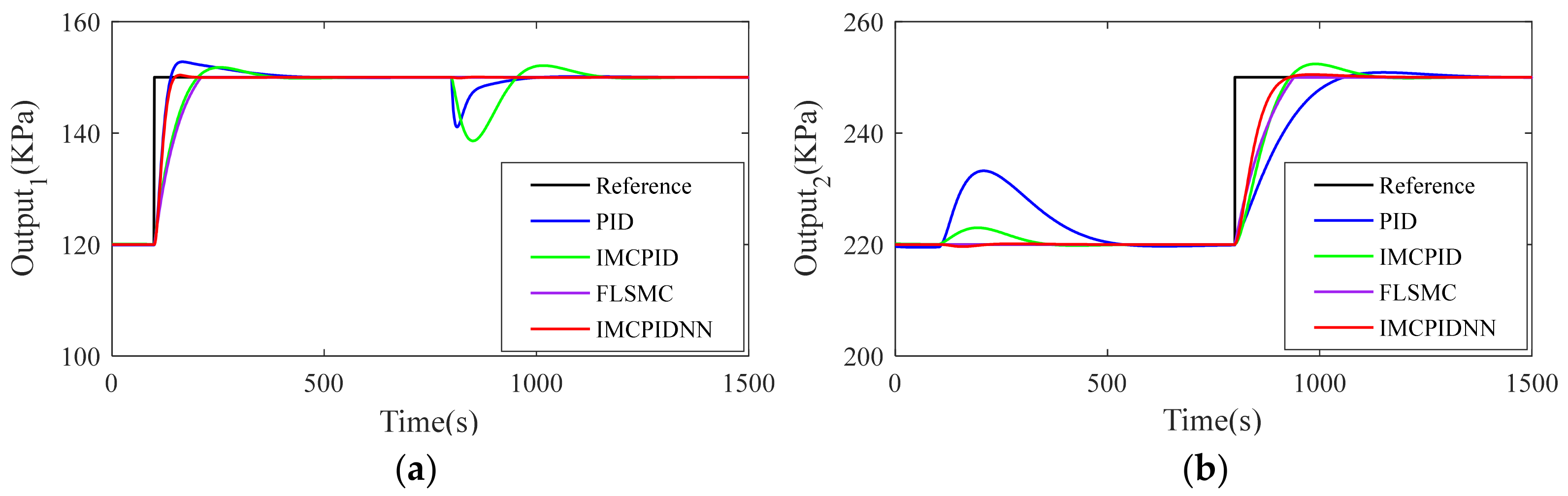
At the moments t = 100 and t = 800, the set-point value is changed sequentially in the two loops. The simulation result in Figure 7 shows the step response and control effect obtained by the proposed IMCPIDNN controller. It is relevant to note that the performance of the PID and IMDPID controllers are not satisfied, and this is expected because of the strong interactions. The common problem of the two controllers is that they cannot eliminate the system coupling problem. For example, the step change at moment t = 100 in the set-point of the first input caused a negative effect on the second output, which is undesirable. It indicates that the system coupling is serious with no decoupling method. The FLSMC controller eliminates the coupling of the system by nonlinear method, but its performance in step response is not as good as that of the IMCPIDNN controller. Compared with the other three controllers, the proposed IMCPIDNN controller performs better in set-point tracking. Neither the first step change nor the second step change has a large effect on the other loop.

The performance comparison of the four algorithms used for sequential step responses are presented in

Table 4. Performance comparison of the four algorithms used for sequential step responses.

Algorithm		${\mathit{M}}_{\mathit{p}} (\%)$	${\mathit{t}}_{\mathit{s}} \left(\mathbf{s}\right)$	IAE(×103)	ISE(×105)	ITAE(×105)	ITSE(×106)
Output1	PID	2.01	85.37	1.01	0.12	7.86	8.80
	IMCPID	0.93	113.68	1.28	0.19	9.62	13.79
	FLSMC	0	53.85	1.02	0.17	7.38	12.52
	IMCPIDNN	0	42.32	0.65	0.12	4.72	8.89
Output2	PID	0.11	182.10	3.20	0.56	47.59	81.71
	IMCPID	0.76	99.97	2.06	0.37	30.18	53.67
	FLSMC	0	83.90	1.56	0.27	22.05	39.57
	IMCPIDNN	0	81.43	1.49	0.27	21.44	38.98

. For loop 1 and 2, the settle times $t_s$ obtained using the proposed controller are 61.91 s and 146.78 s respectively, and the overshoots ${\mathit{M}}_{\mathit{p}}$ are both zero. Meanwhile, the results of the smallest four error evaluation indexes obtained by the IMCPIDNN controller can ensure the set-point tracking accuracy. Obviously, the IMCPIDNN controller performs better in terms of facing the interactions.

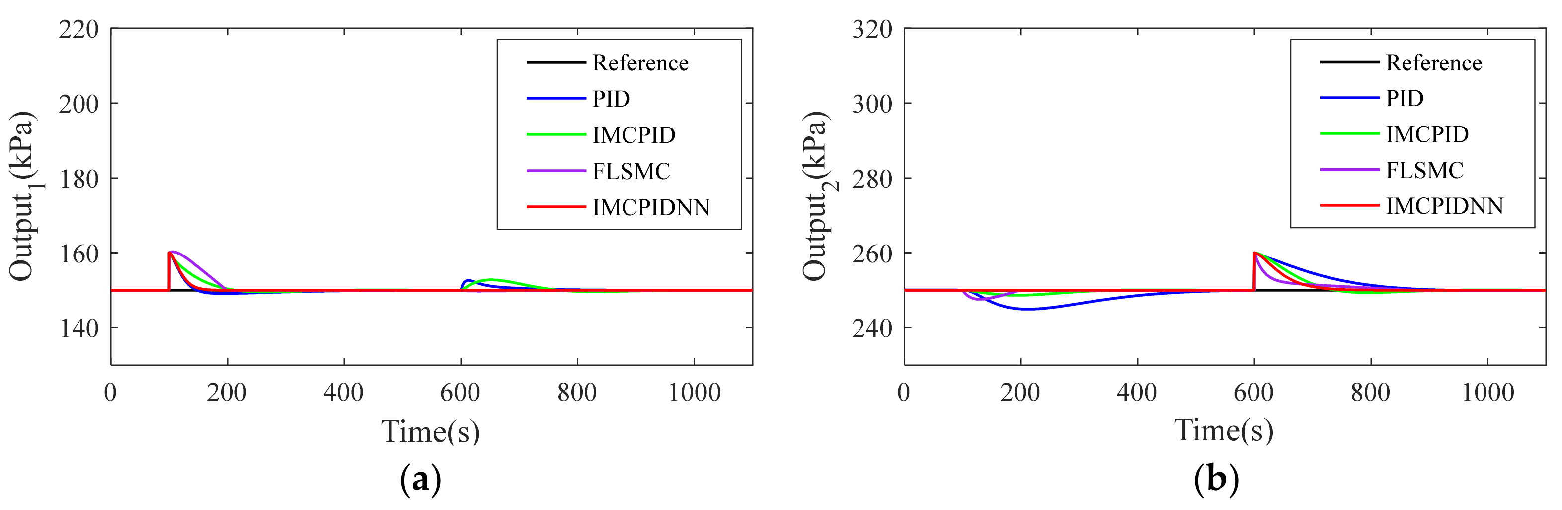
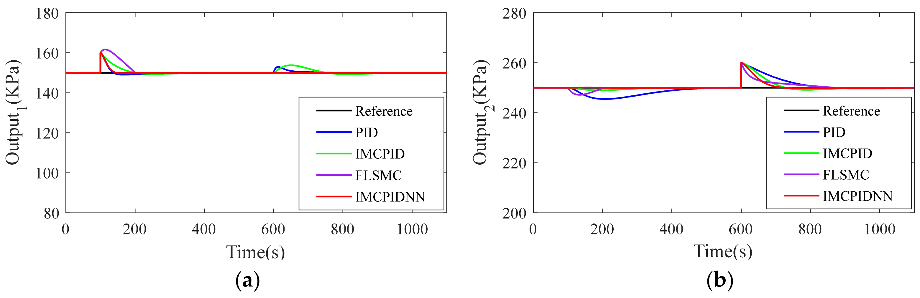
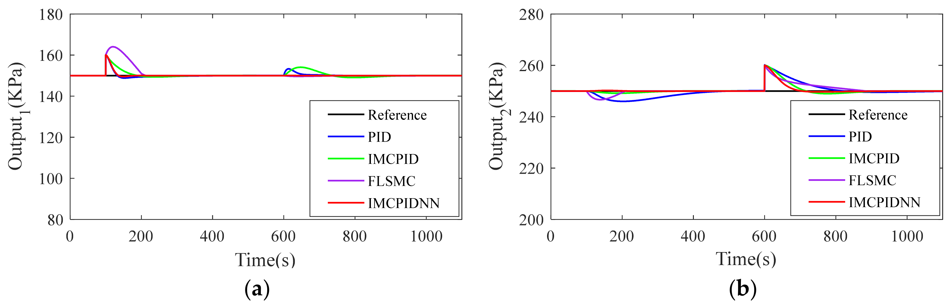
4.2. Anti-Interference and Robustness Test

To illustrate the stability of the proposed IMCPIDNN controller, some anti-interference and robustness tests had been done. We want to know how the control effect changes when the values of the transfer function time constant and gain are mismatched with the actual system and how these controllers perform when the control process encounters external disturbance.

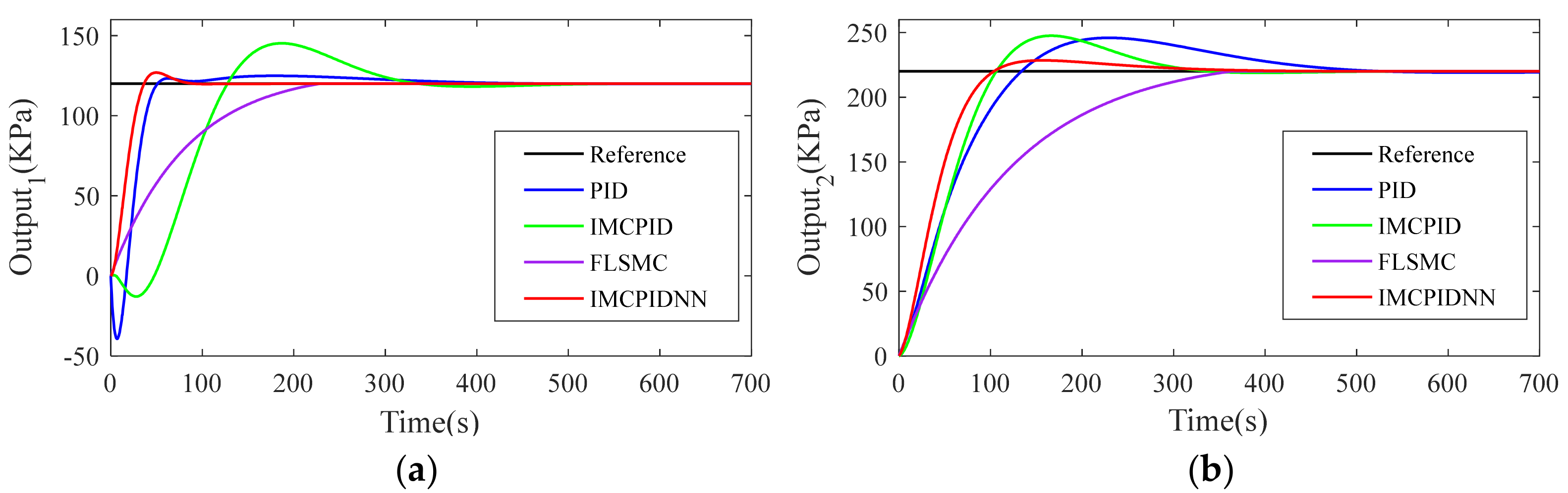
Figure 8 and Figure 9 present the step response with +40% variation on time constant and gains. We can see that the proposed IMCNNPID controller is very stable to the changes of model parameters. Figure 8 shows that the overshoot of PID, IMCPID, FLSM and IMCPIDNN in the face of model mismatch is 3.60%, 16.59%, 0% and 1.79%, respectively. Additionally, it can be seen that the IMCPIDNN controller has a faster adjustment speed than the other three controllers. 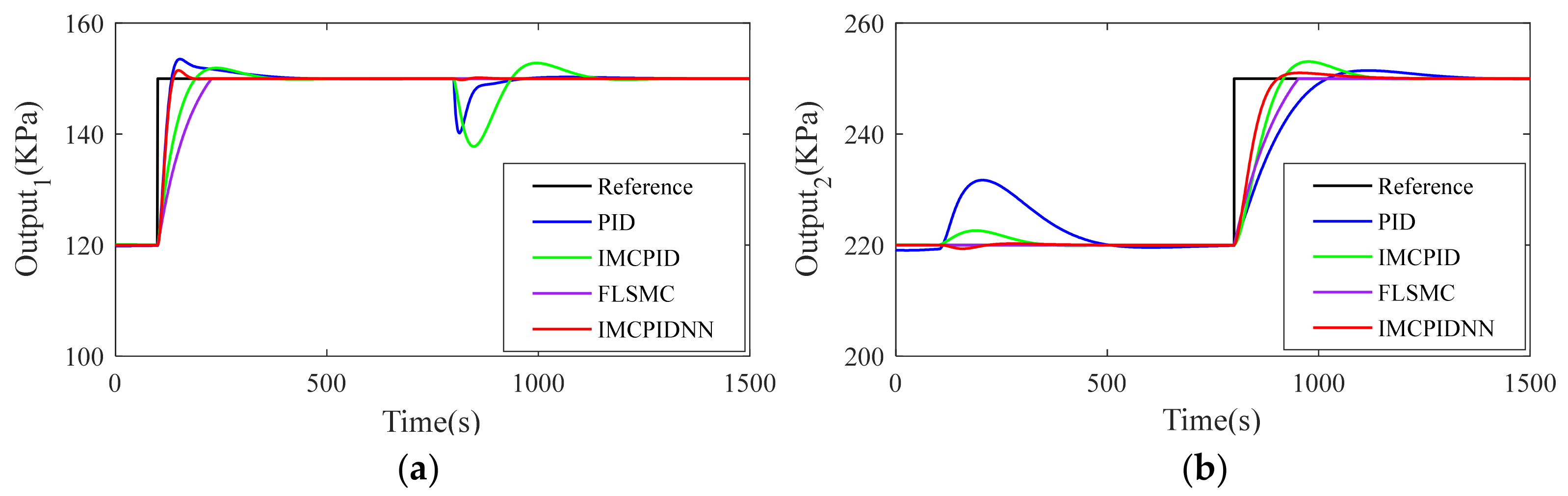Figure 9 shows the process outputs when the model mismatch increases to +40%. The most interesting aspect of these two figures is that the overshoot obtained by the IMCPIDNN controller is slightly larger than Figure 10 and Figure 11, but it is acceptable because it is still small enough. Obviously, the proposed IMCPIDNN controller is effective and superior to other three controllers for the varied system errors.

Next, 20 kPa of external disturbance was added to output 1 and output 2 at t = 100 s and t = 600 s, respectively. The simulation results are shown in Figure 12, Figure 13, Figure 14. Compared with the PID, IMCPID and FLSMC controllers, the settle time and overshoot of the proposed IMCPIDNN controller performed better, obviously. Under the action of the IMCPIDNN controller, the output can return to the set-point faster and more steadily, and the other loop is not interfered. This is meaningful for a stepless flow control system as it can ensure that the system runs more safely in the presence of external interference and reduce the failure rate of the equipment.

5. Conclusions

In this paper, an IMCPIDNN controller based on IMCPID and a neural network optimization algorithm is proposed to optimize the control effect of MIMO processes such as stepless flow control of reciprocating compressors. The main contributions of this paper are the stepless flow process model with dynamic parameters as well as an IMCPIDNN controller, which inherits the main structure of a PID controller. In order to adjust the control parameters more efficiently, an adaptive algorithm based on a BP neural network is constructed. In terms of efficiently adjusting control parameters, the BP neural network algorithm with dynamically adjustable parameters has played a key role. Numerical experiments show that the proposed IMCPIDNN controller has good setpoint tracking performance and adaptability to a system model mismatch. Compared with PID, IMCPID and FLSMC controllers under the same conditions, the proposed IMCPIDNN controller performs best in terms of settle time, overshoot, robustness and anti-interference ability. More importantly, the process of the proposed IMCPIDNN controller to adjust the control parameters is the simplest because of the fewest adjustable parameters, which will provide great convenience for actual industrial applications. Finally, the proposed controller can be applied to any linear or non-linear MIMO system. We will continue to study process modeling, stability analysis, system convergence and robustness analysis to achieve better control effects.