
Machine Learning for the Identification of Hydration Mechanisms of Pharmaceutical-Grade Cellulose Polymers and Their Mixtures with Model Drugs


Abstract
:1. Introduction
2. Materials and Methods
2.1. DSC Studies
- the water concentrations of the hydrated samples under study were expressed as Wc, although Wc is defined as the water fraction mH2O related the to dry mass mdry of raw HPC or an HPC mixture (Wc = mH2O/mdry)
- the decomposition of the curves was used for the DSC plots, from the lowest to the highest hydration level Wc
- only melting peaks were used for decomposition analysis
- the amount of NFW water calculated for raw HPC was equal to 0.54 g/g, which is comparable to the amount calculated for HPC/NaSA 0.48 g/g
- NFW calculated for HPC/SA was equal to 0.18 g/g, which is almost 1/3 of the NFW amount measured for raw HPC and the HPC/NaSA mixture
- for water contents below NFW, all water found in the matrix is considered non-freezing NFW
- below the NFW value, the melting peaks for raw HPC and its mixtures are not visible in the DSC measurements; for that reason, the decomposition procedure was performed only for samples with a water concentration Wc > NFW, usually, above 0.7–0.8 g/g
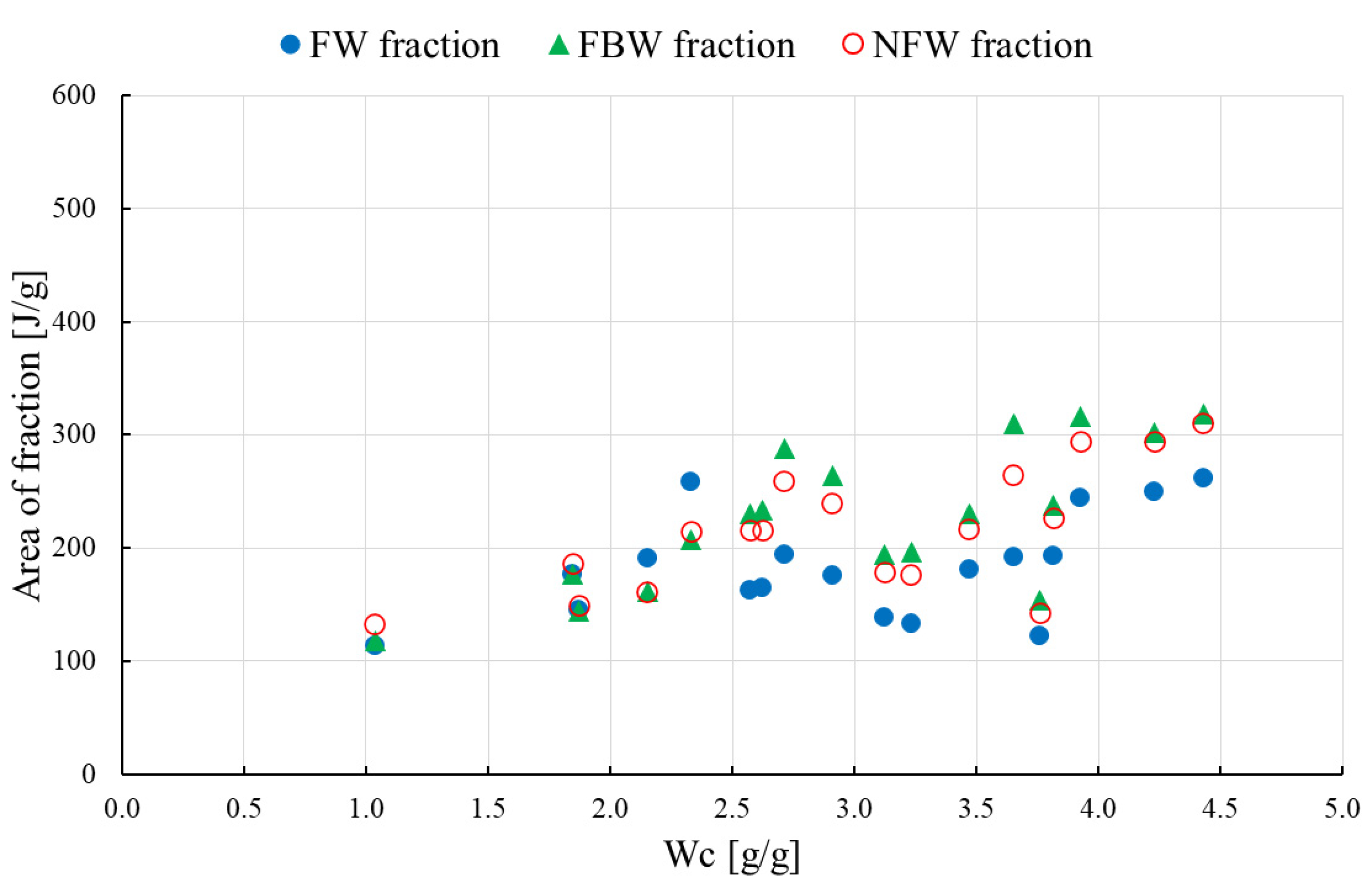
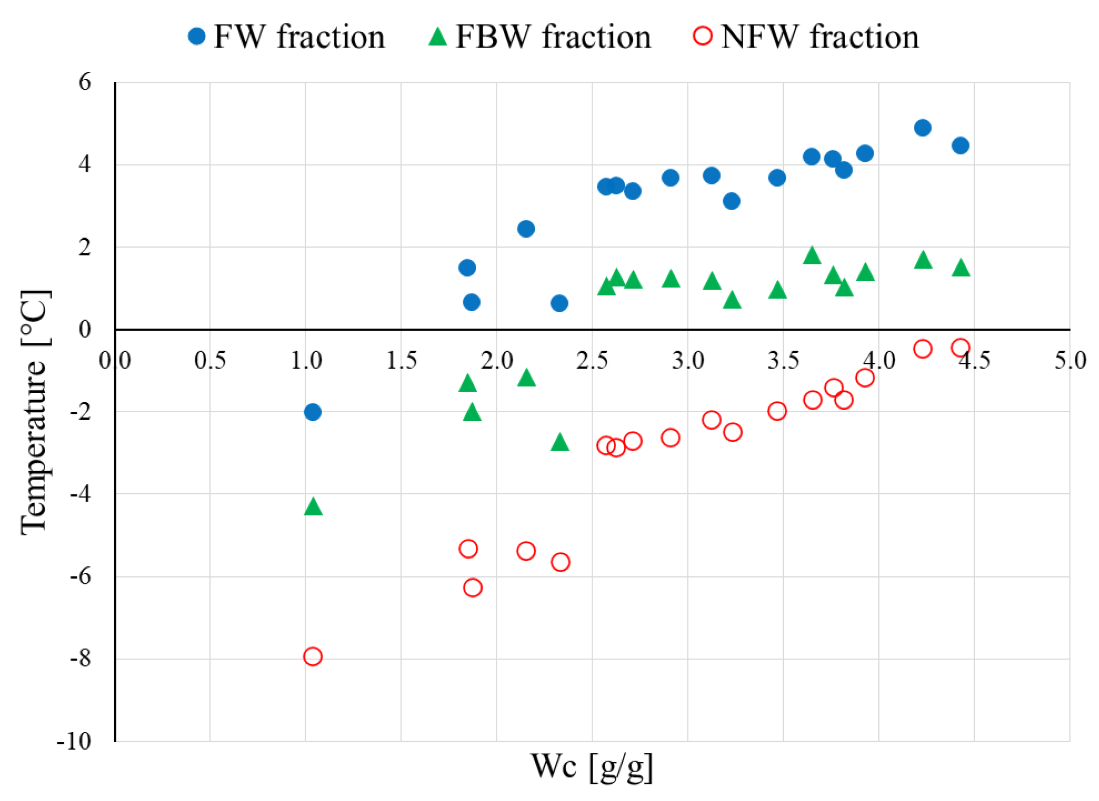
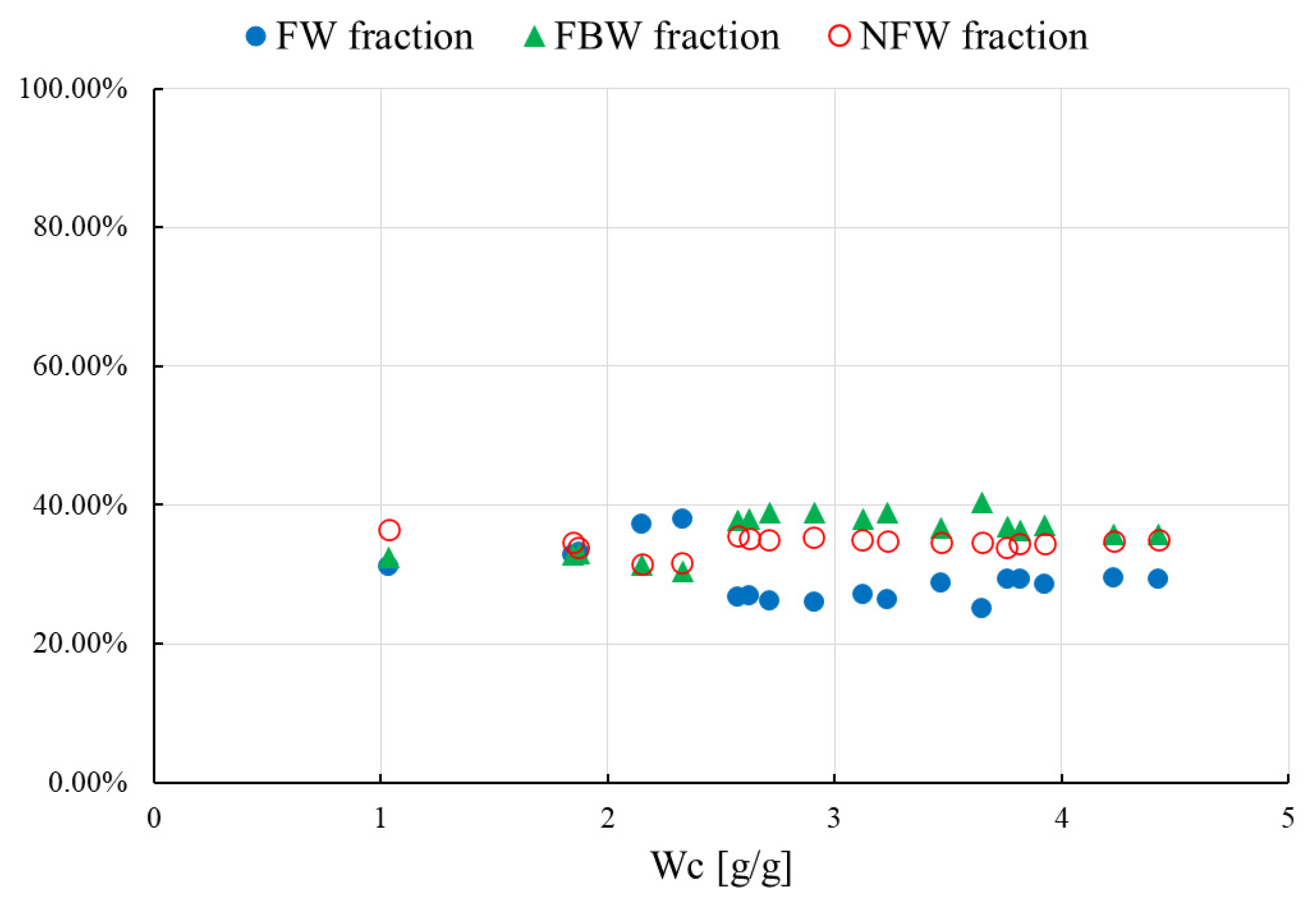
- the weight of freezing-bound FBW and non-freezing NFW water per g HPC or HPC/mixture is constant
- the developed model should consider the contribution of specific nanostructures, the so-called nanocavities, in water holding
- the developed model should consider the strong dissociative effect of the Na+ cation
2.2. Curve Decomposition Tool
- -
- nloptr
- -
- GenSA
- -
- rgenoud
- -
- optimx
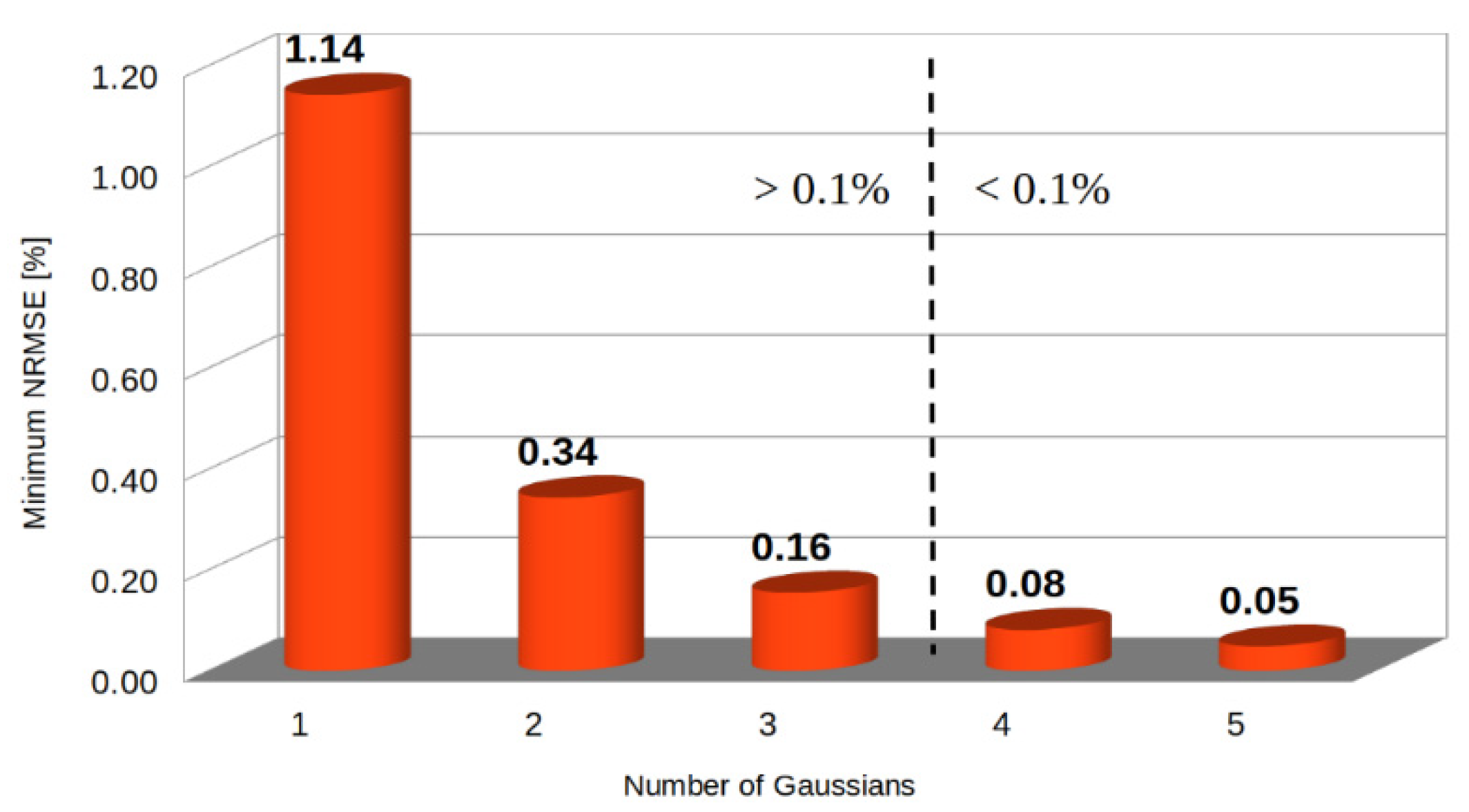
- following Occam’s razor, the number of components curves should be minimal
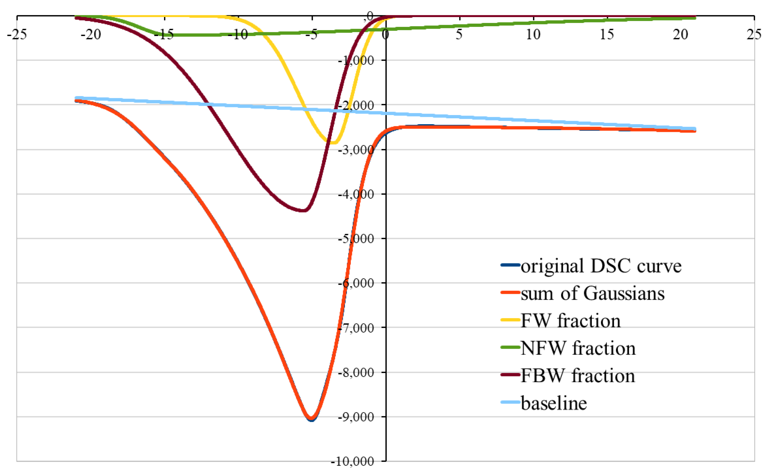
- since the ice-melting curves were asymmetrical, they were deconvoluted using bi-Gaussian functions
- the theoretical curve given by the sum of the individual ones was best fitted to the experimental DSC curve
- the goodness-of-fit criterion was normalized root-mean-squared error (NRMSE) calculated according to the formula in Equation (2); an empirical rule of NRMSE < 0.1% was employed as an algorithm stopping criterion.
3. Results and Discussion
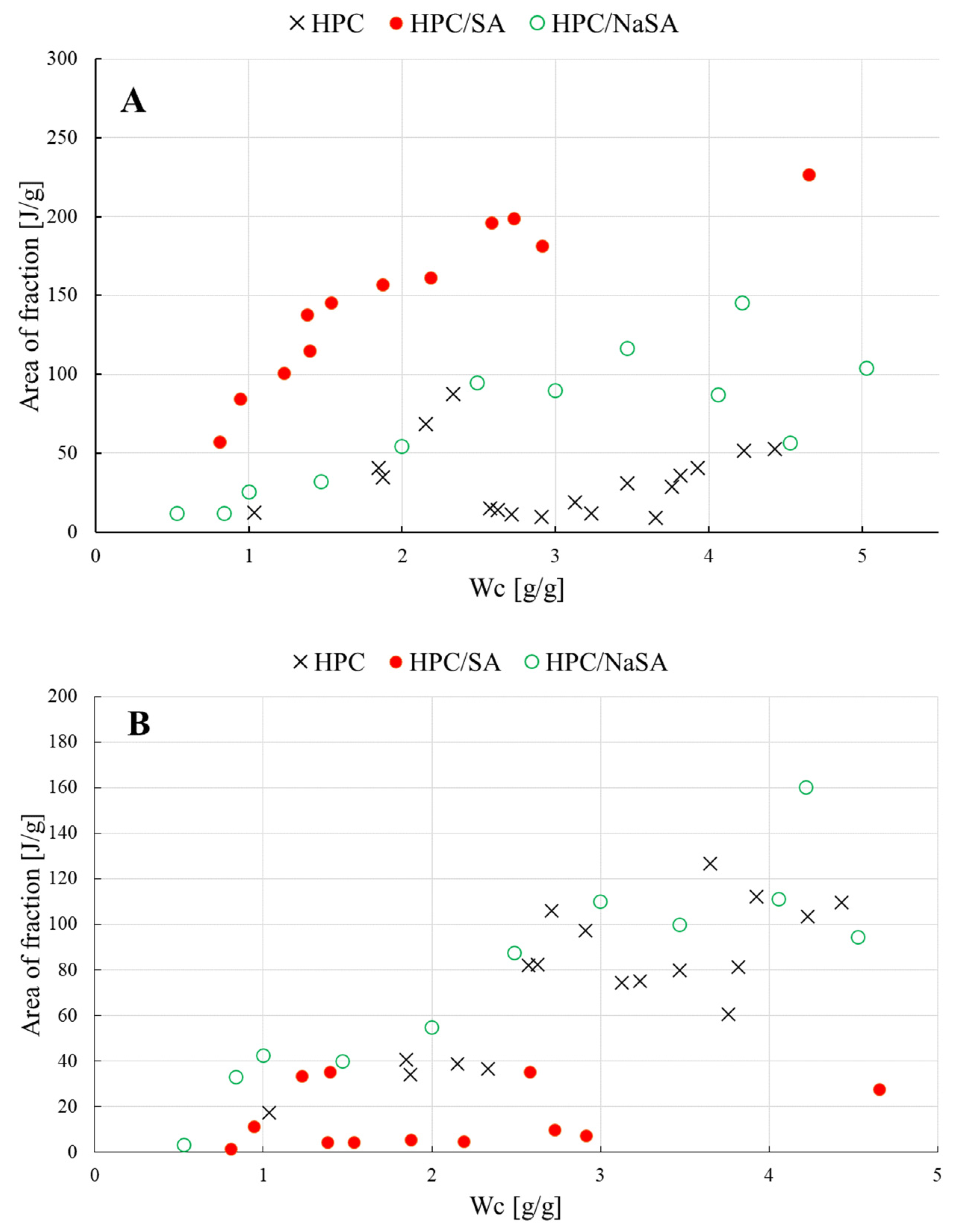
3.1. Search for the Optimum Number of Gaussian Components
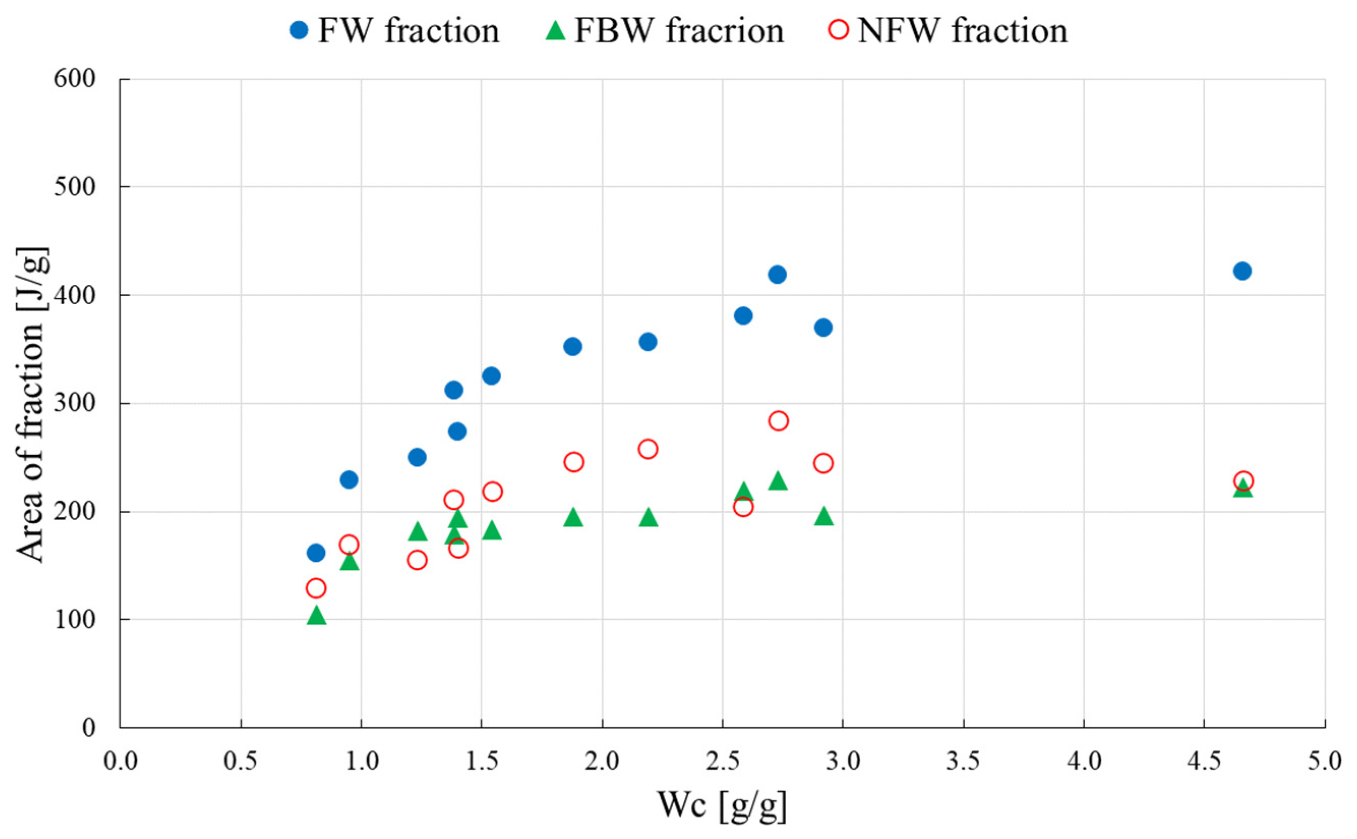
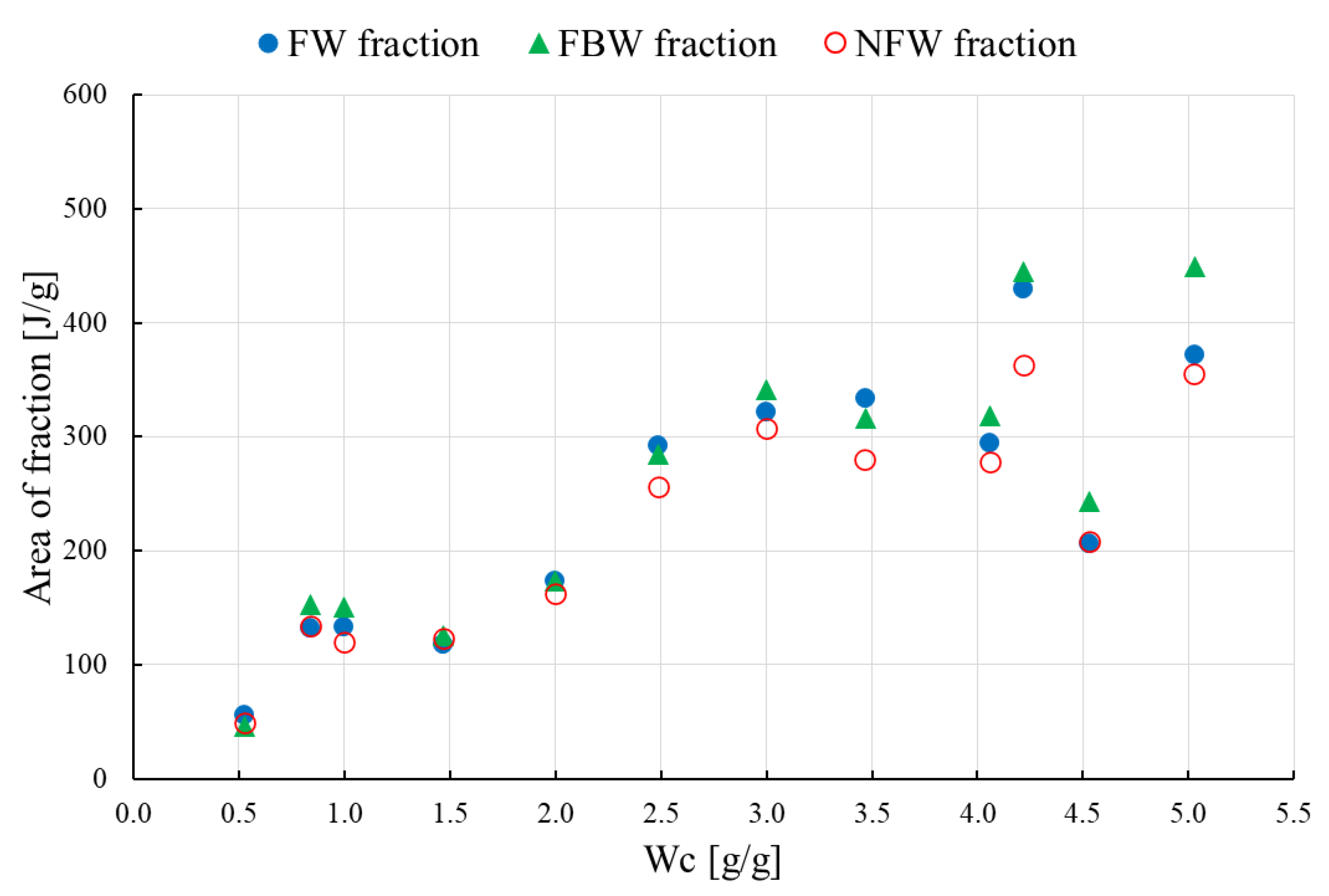
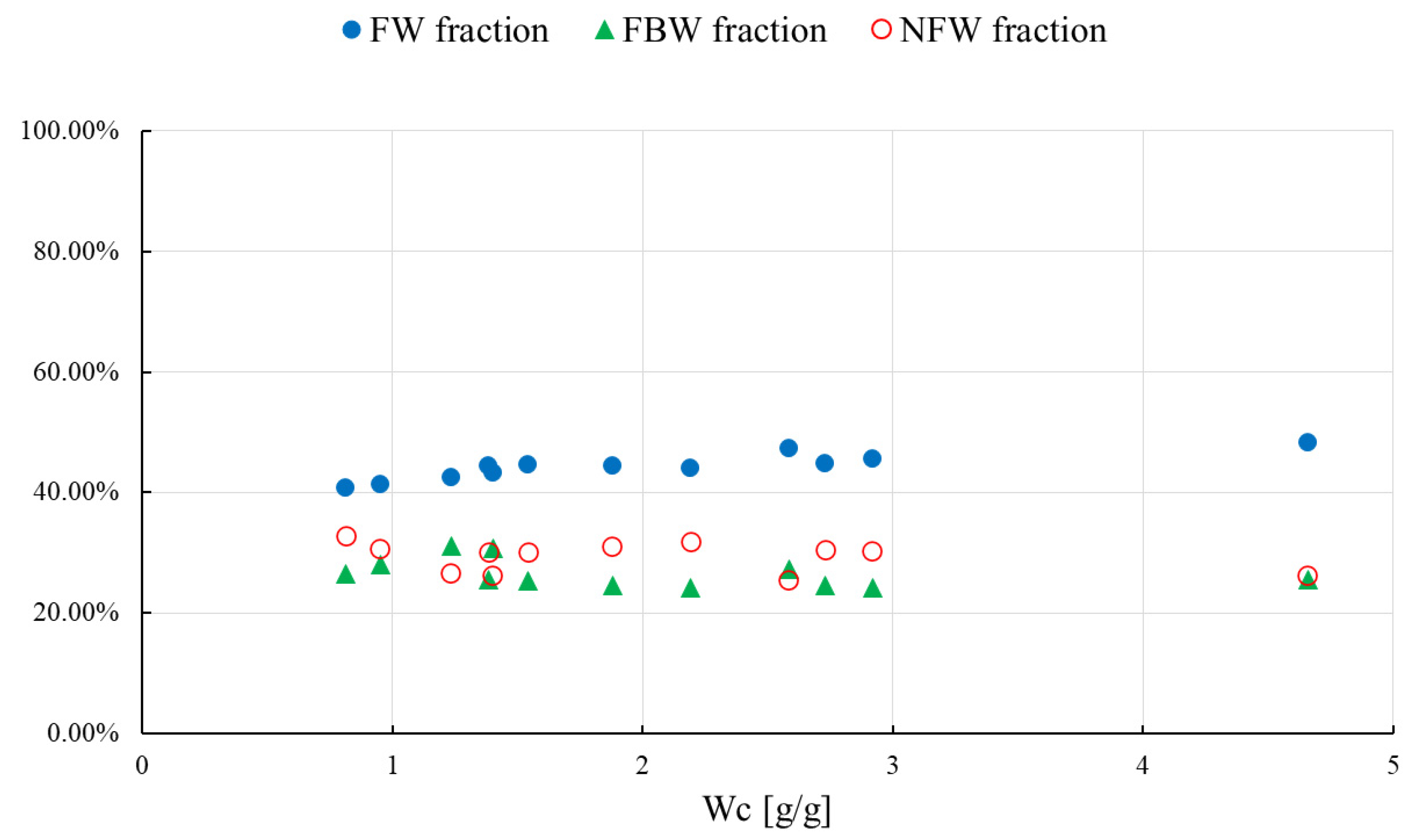
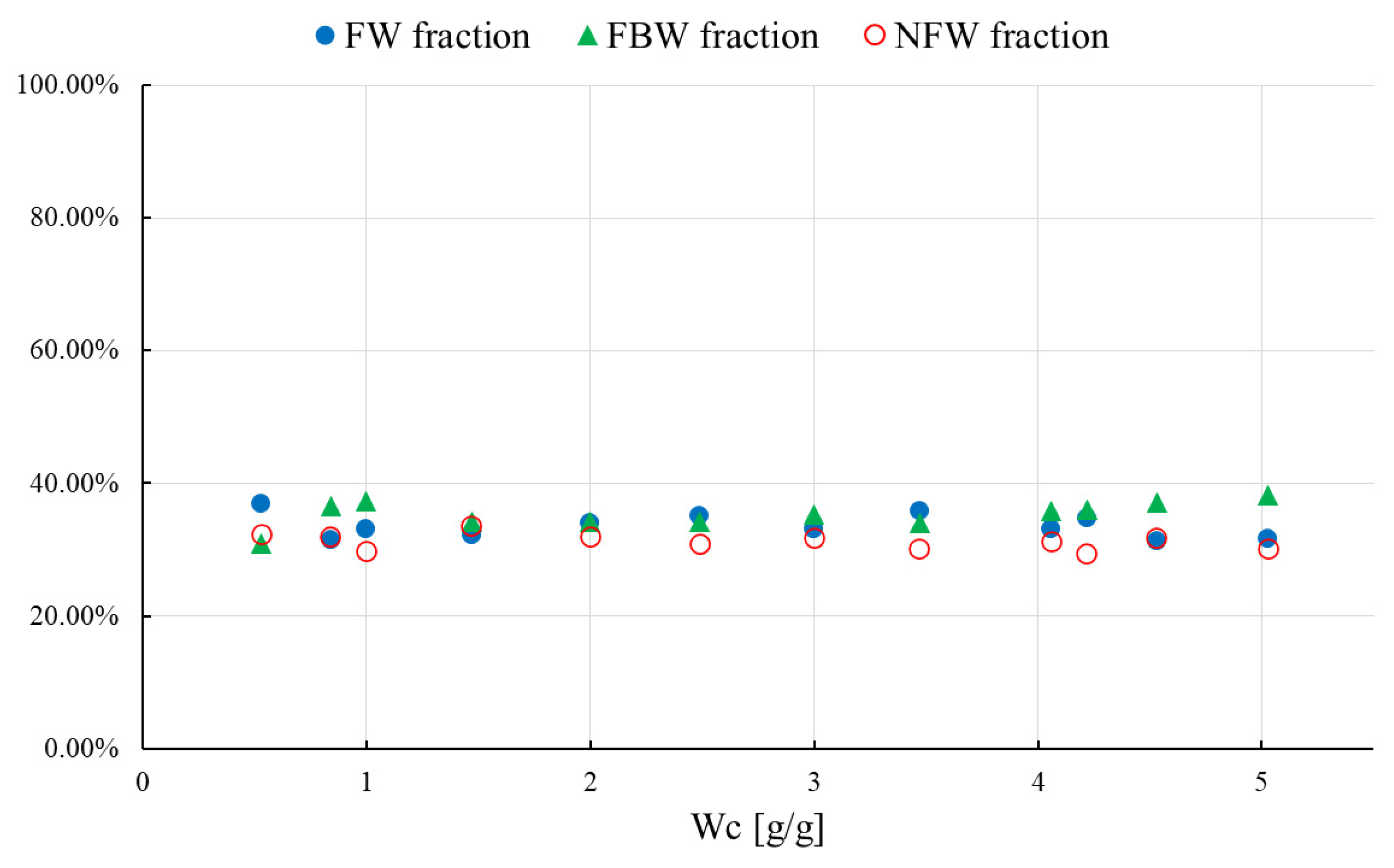
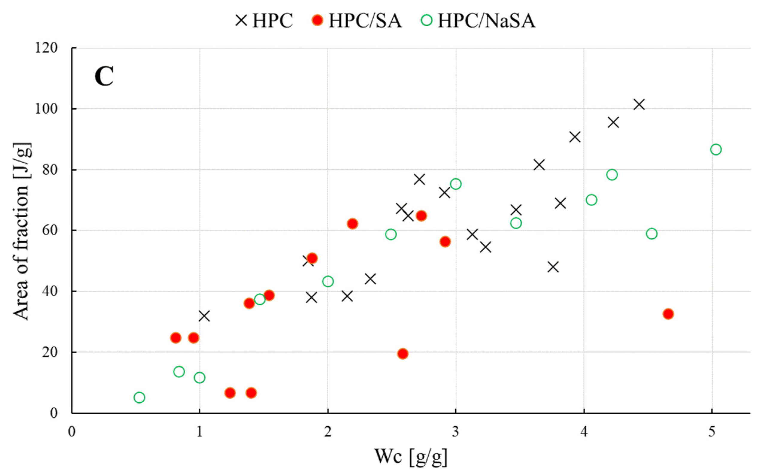
3.2. Three-Component Analysis
4. Conclusions
- assigning the maximum temperatures Tmax to the empirically determined components allowed confirming the identity of each water fraction—the same conclusions regarding the relationship Tmax vs. Wc, but obtained from raw, not decomposed DSC curves, were the subject of another publication [20]
- -
- the development and publication of the AI/ML tool for the decomposition of DSC curves as an open source software freely available both for personal and for commercial use [28]
- -
- the proof-of-concept use of the above-mentioned tool for DSC results for HPC/water mixtures with model drugs
- -
- the confirmation of some AI/ML empirically developed hypotheses in the literature about the thermal behavior of HPC/water mixtures
Author Contributions
Funding
Institutional Review Board Statement
Informed Consent Statement
Data Availability Statement
Conflicts of Interest
Abbreviations
| PAT | process analytical technologies |
| QbD | quality by design |
| DSC | differential scanning calorimetry |
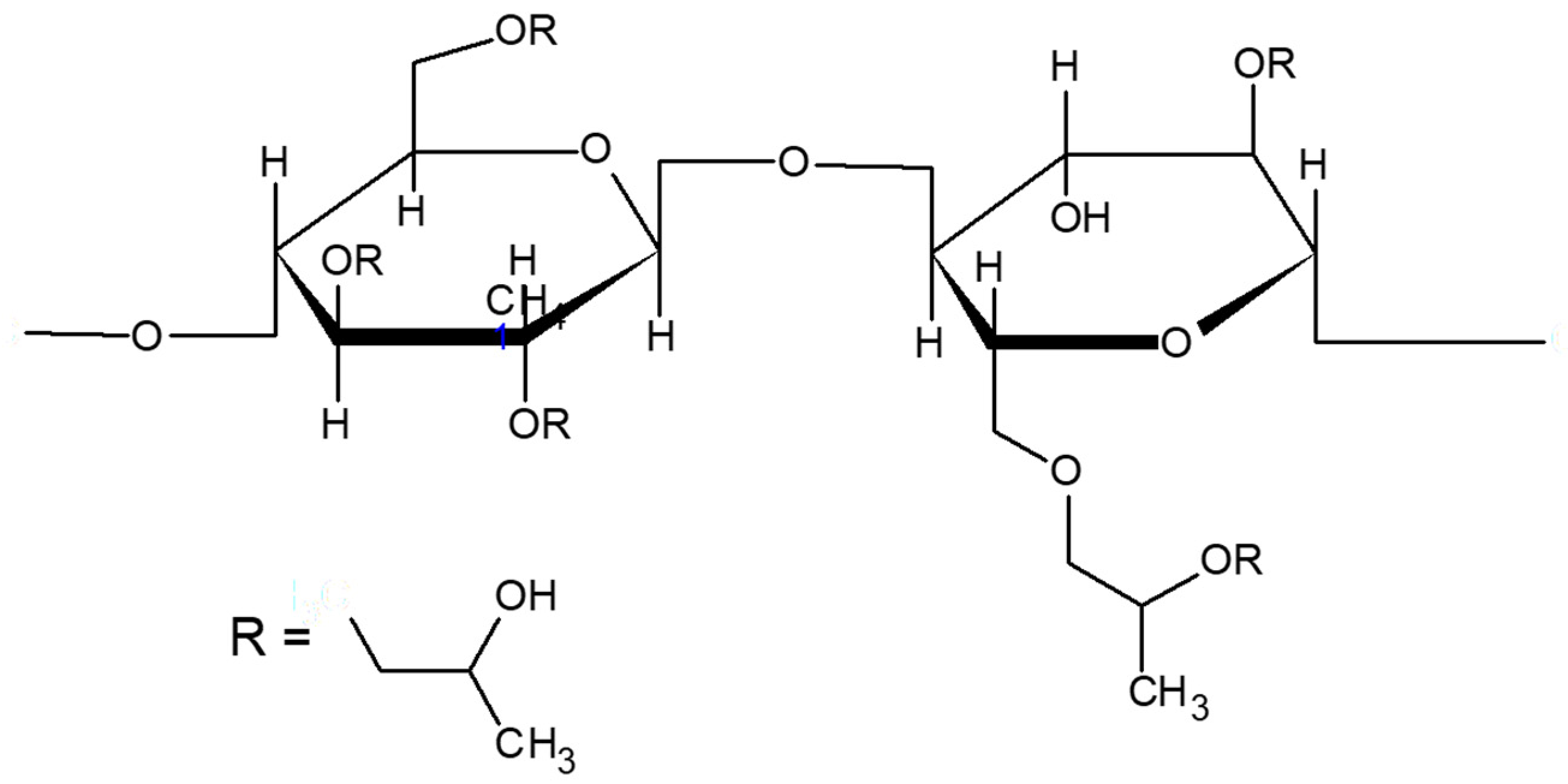
| HPC | hydroxypropyl cellulose |
| FW | free (or bulk) water |
| FBW | freezing bound water |
| NFW | non-freezing bound water |
| SA | salicylic acid |
| NaSA | sodium salicylate |
| HPC/SA | a binary physical mixture of hydroxypropyl cellulose and salicylic acid 1:1 w/w |
| HPC/NaSA | a binary physical mixture of hydroxypropyl cellulose and sodium salicylate 1:1 w/w |
| BFGS | Broyden–Fletcher–Goldfarb–Shanno (BFGS) algorithm is an iterative method for solving unconstrained nonlinear optimization problems |
| LADME | Liberation, Absorption, Distribution, Metabolism, Excretion—major processes responsible for drugs behavior in the human body. |
References
- ICH. The International Conference on Harmonization of Technical Requirements for Registration of Pharmaceuticals for Human Use, Quality Guideline Q8(R2) Pharmaceutical Development. 2009. Available online: http://www.ich.org/fileadmin/Public_Web_Site/ICH_Products/Guidelines/Quality/Q8_R1/Step4/Q8_R2_Guideline.pdf (accessed on 21 June 2021).
- Clas, S.D.; Dalton, C.R.; Hancock, B.C. Differential scanning calorimetry: Applications in drug development. Pharm. Sci. Technol. Today 1999, 2, 311–320. [Google Scholar] [CrossRef]
- Witika, B.A.; Aucamp, M.; Mweetwa, L.L.; Makoni, P.A. Application of Fundamental Techniques for Physicochemical Characterizations to Understand Post-Formulation Performance of Pharmaceutical Nanocrystalline Materials. Crystals 2021, 11, 310. [Google Scholar] [CrossRef]
- Knopp, M.M.; Löbmann, K.; Elder, D.P.; Rades, T.; Holm, R. Recent advances and potential applications of modulated differential scanning calorimetry (mDSC) in drug development. Eur. J. Pharm. Sci. 2016, 87, 164–173. [Google Scholar] [CrossRef] [PubMed]
- Leyva-Porras, C.; Cruz-Alcantar, P.; Espinosa-Solís, V.; Martínez-Guerra, E.; Piñón-Balderrama, C.I.; Compean Martínez, I.; Saavedra-Leos, M.Z. Application of Differential Scanning Calorimetry (DSC) and Modulated Differential Scanning Calorimetry (MDSC) in Food and Drug Industries. Polymers 2020, 12, 5. [Google Scholar] [CrossRef] [Green Version]
- Bernardes, C.E.S.; Joseph, A.; Minas da Piedade, M.E. Some practical aspects of heat capacity determination by differential scanning calorimetry. Thermochim. Acta 2020, 687, 178574. [Google Scholar] [CrossRef]
- Faroongsarng, D. Theoretical Aspects of Differential Scanning Calorimetry as a Tool for the Studies of Equilibrium Thermodynamics in Pharmaceutical Solid Phase Transitions. AAPS PharmSciTech 2016, 17, 572–577. [Google Scholar] [CrossRef] [PubMed]
- Aloisio, C.; Gomes De Oliveira, A.; Longhi, M. Characterization, inclusion mode, phase-solubility and in vitro release studies of inclusion binary complexes with cyclodextrins and meglumine using sulfamerazine as model drug. Drug Dev. Ind. Pharm. 2014, 40, 919–928. [Google Scholar] [CrossRef] [PubMed]
- Talik, P.; Żuromska-Witek, B.; Hubicka, U.; Krzek, J. The use of the DSC method in quantification of active pharmaceutical ingredients in commercially available one component tablets. Acta Pol. Pharm. 2017, 74, 1049–1055. [Google Scholar]
- Wyttenbach, N.; Niederquell, A.; Kuentz, M. Machine Estimation of Drug Melting Properties and Influence on Solubility Prediction. Mol Pharm. 2020, 17, 2660–2671. [Google Scholar] [CrossRef]
- Picker-Freyer, K.M.; Durig, T. Physical mechanical and tablet formation properties of hydroxypropylcellulose: In pure form and in mixtures. AAPS PharmSciTech 2007, 8, 82–90. [Google Scholar] [CrossRef] [Green Version]
- Arca, H.C.; Mosquera-Giraldo, L.I.; Bi, V.; Xu, D.; Taylor, L.S.; Edgar, K.J. Pharmaceutical applications of cellulose ethers and cellulose ether esters. Biomacromolecules 2018, 19, 2351–2376. [Google Scholar] [CrossRef] [PubMed]
- Klose, R.E.; Glickman, M. Gums. In Handbook of Food Additives, 2nd ed.; Furia, T.E., Ed.; CRC Press: Boca Raton, FL, USA, 1973; Volume 1, pp. 295–360. [Google Scholar]
- Tanaka, A.; Furubayashi, T.; Tomisaki, M.; Kawakami, M.; Kimura, S.; Inoue, D.; Kusamori, K.; Katsumi, H.; Sakane, T.; Yamamoto, A. Nasal drug absorption from powder formulations: The effect of three types of hydroxypropyl cellulose (HPC). Eur. J. Pharm. Sci. 2017, 96, 284–289. [Google Scholar] [CrossRef]
- Macchi, E.; Zema, L.; Pandey, P.; Gazzaniga, A.; Felton, L.A. Influence of temperature and relative humidity conditions on the pan coating of hydroxypropyl cellulose molded capsules. Eur. J. Pharm. Biopharm. 2016, 100, 47–57. [Google Scholar] [CrossRef] [PubMed]
- Hughey, J.R.; Keen, J.M.; Bennett, R.C.; Obara, S.; McGinity, J.W. The incorporation of low-substituted hydroxypropyl cellulose into solid dispersion systems. Drug Dev. Ind. Pharm. 2015, 41, 1294–1301. [Google Scholar] [CrossRef] [PubMed]
- Mlčoch, T.; Kučerík, J. Hydration and drying of various polysaccharides studied using DSC. J. Therm. Anal. Calorim. 2013, 113, 1177–1185. [Google Scholar] [CrossRef]
- Ping, Z.H.; Nguyen, Q.T.; Chen, S.M.; Zhou, J.Q.; Ding, Y.D. States of water in different hydrophilic polymers—DSC and FTIR studies. Polymer 2001, 42, 8461–8467. [Google Scholar] [CrossRef]
- Hatakeyama, T.; Inui, Y.; Iijima, M.; Hatakeyama, H. Bound water restrained by nanocellulose fibres. J. Therm. Anal. Calorim. 2013, 113, 1019–1025. [Google Scholar] [CrossRef]
- Talik, P.; Hubicka, U. The DSC approach to study non-freezing water contents of hydrated hydroxypropylcellulose (HPC): A study over effects of viscosity and drug addition. J. Therm. Anal. Calorim. 2018, 132, 445–451. [Google Scholar] [CrossRef] [Green Version]
- Talik, P.; Hubicka, U. A study of the drying behaviour of various types of hydrated hydroxypropyl cellulose (HPC) and their mixtures with drugs of different solubility using DSC. J. Therm. Anal. Calorim. 2021, 143, 247–254. [Google Scholar] [CrossRef]
- Singh, B.; Chauhan, G.S.; Sharma, D.K.; Kant, A.; Gupta, I.; Chauhan, N. The release dynamics of model drugs from the psyllium and N-hydroxymethylacrylamide based hydrogels. Int. J. Pharm. 2006, 325, 15–25. [Google Scholar] [CrossRef]
- Pade, V.; Stavchansky, S. Estimation of the Relative Contribution of the Transcellular and Paracellular Pathway to the Transport of Passively Absorbed Drugs in the Caco-2 Cell Culture Model. Pharm. Res. 1997, 14, 1210–1215. [Google Scholar] [CrossRef] [PubMed]
- Tungprapa, S.; Jangchud, I.; Supaphol, P. Release characteristics of four model drugs from drug-loaded electrospun cellulose acetate fiber mats. Polymer 2007, 48, 5030–5041. [Google Scholar] [CrossRef]
- Taepaiboon, P.; Rungsardthong, U.; Supaphol, P. Drug-loaded electrospun mats of poly(vinyl alcohol) fibres and their release characteristics of four model drugs. Nanotechnology 2006, 17, 2317–2329. [Google Scholar] [CrossRef]
- Brehm, M.; Pulst, M.; Kressler, J.; Sebastiani, D. Triazolium-Based Ionic Liquids: A Novel Class of Cellulose Solvents. J. Phys. Chem. B 2019, 123, 3994–4003. [Google Scholar] [CrossRef] [Green Version]
- Brehm, M.; Radicke, J.; Pulst, M.; Shaabani, F.; Sebastiani, D.; Kressler, J. Dissolving Cellulose in 1,2,3-Triazolium- and Imidazolium-Based Ionic Liquids with Aromatic Anions. Molecules 2020, 25, 3539. [Google Scholar] [CrossRef] [PubMed]
- R Peak Decomposer. Available online: https://sourceforge.net/projects/r-peak-decomposer (accessed on 21 June 2021).
- R Interface to NLopt. Available online: https://cran.r-project.org/package=nloptr (accessed on 21 June 2021).
- Generalized Simulated Annealing. Available online: https://cran.r-project.org/package=GenSA (accessed on 21 June 2021).
- R Version of GENetic Optimization Using Derivatives. Available online: https://cran.r-project.org/package=rgenoud (accessed on 21 June 2021).
- R Optimx Package. Available online: https://cran.r-project.org/package=optimx (accessed on 21 June 2021).
- Kaelo, P.; Ali, M.M. Some variants of the controlled random search algorithm for global optimization. J. Optim. Theory Appl. 2006, 130, 253–264. [Google Scholar] [CrossRef]
- Xiang, Y.; Gubian, S.; Suomela, B.; Hoeng, J. Generalized Simulated Annealing for Efficient Global Optimization: The GenSA Package for R. R J. 2013, 5, 13–28. Available online: https://journal.r-project.org/archive/2013/RJ-2013-002/index.html (accessed on 21 June 2021). [CrossRef] [Green Version]
- Walter, R.; Mebane, J.; Sekhon, J.S. Genetic Optimization Using Derivatives: The rgenoud Package for R. J. Stat. Softw. 2011, 42, 1–26. Available online: http://www.jstatsoft.org/v42/i11/ (accessed on 21 June 2021).
- Nash, J.C.; Varadhan, R. Unifying Optimization Algorithms to Aid Software System Users: Optimx for R. J. Stat. Softw. 2011, 43, 1–14. Available online: https://www.jstatsoft.org/v43/i09/ (accessed on 21 June 2021). [CrossRef] [Green Version]
- Liu, G.L.; Yao, K.D. What causes the unfrozen water in polymers: Hydrogen bonds between water and polymer chains? Polymer 2001, 42, 3943–3947. [Google Scholar] [CrossRef]
- Talik, P.; Moskal, P.; Proniewicz, L.M.; Wesełucha-Birczyńska, A. The Raman spectroscopy approach to the study of Water–Polymer interactions in hydrated hydroxypropyl cellulose (HPC). J. Mol. Struct. 2020, 1210, 128062. [Google Scholar] [CrossRef]
- Park, S.; Venditti, R.A.; Jameel, H.; Pawlak, J.J. Studies of the heat of vaporization of water associated with cellulose fibres characterized by thermal analysis. Cellulose 2007, 14, 195–204. [Google Scholar] [CrossRef]
- Berthold, J.; Desbrieres, J.; Rinaudo, M.; Salmén, L. Types of adsorbed water in relation to the ionic groups and their counter-ions for some cellulose derivatives. Polymer 1994, 35, 5729–5736. [Google Scholar] [CrossRef]


Publisher’s Note: MDPI stays neutral with regard to jurisdictional claims in published maps and institutional affiliations. |
© 2021 by the authors. Licensee MDPI, Basel, Switzerland. This article is an open access article distributed under the terms and conditions of the Creative Commons Attribution (CC BY) license (https://creativecommons.org/licenses/by/4.0/).
Share and Cite
Talik, P.; Mendyk, A. Machine Learning for the Identification of Hydration Mechanisms of Pharmaceutical-Grade Cellulose Polymers and Their Mixtures with Model Drugs. Appl. Sci. 2021, 11, 7751. https://doi.org/10.3390/app11167751
Talik P, Mendyk A. Machine Learning for the Identification of Hydration Mechanisms of Pharmaceutical-Grade Cellulose Polymers and Their Mixtures with Model Drugs. Applied Sciences. 2021; 11(16):7751. https://doi.org/10.3390/app11167751
Chicago/Turabian StyleTalik, Przemysław, and Aleksander Mendyk. 2021. "Machine Learning for the Identification of Hydration Mechanisms of Pharmaceutical-Grade Cellulose Polymers and Their Mixtures with Model Drugs" Applied Sciences 11, no. 16: 7751. https://doi.org/10.3390/app11167751
APA StyleTalik, P., & Mendyk, A. (2021). Machine Learning for the Identification of Hydration Mechanisms of Pharmaceutical-Grade Cellulose Polymers and Their Mixtures with Model Drugs. Applied Sciences, 11(16), 7751. https://doi.org/10.3390/app11167751