Optimal Control of a Virtual Power Plant by Maximizing Conditional Value-at-Risk

Abstract

This research acquired data from the Central Weather Bureau Observation Data Inquiry System (CODIS) for historical weather information, such as observation time, temperature, humidity, wind speed, global radiation, etc., and constructed a historical weather database by using Excel software. Least square support vector machine (LSSVM) was used to forecast wind speed and solar radiation; then, the power output of wind and solar was derived. Considering factors of the demand response and the load and electricity pricing, a maximized risk income model of the virtual power plant (VPP) is established based on conditional value-at-risk (CVAR). An enhanced bacterial foraging algorithm (EBFA) was proposed to solve the risk dispatch problem of a VPP in this paper. In an EBFA, the stochastic weight trade-off is embedded to improve the behavior pattern of individual bacteria to enhance their sorting efficiency and accuracy in a high-dimension solution space. Various moving patterns of EBFA were considered for improvement, which were demonstrated by using a VPP system on Penghu island, Taiwan. Many scenarios were created, including various seasons, power rebate pricings, and confidence levels, so the maximal risk and return of VPP could be simulated and analyzed. Simulation and tests show a positive result for a VPP to perform the power dispatch by maximizing risk income. This paper also provides a guideline for the VPP to handle the risk management.

1. Introduction

Climate change due to the greenhouse effect is a major topic in studying the increasingly serious problem of global warming. Controlling greenhouse gases is an important gateway for international organizations to perform environmental protection. The use of distributed energy resources (DERs) is a popular trend for friendly energy dispatch in reducing greenhouse gases. They are generally close to the load and can improve power quality and reliability [1]. DERs refer to distributed generations (DGs), including renewable energy and energy storage systems (ESS), which require a dispatch strategy to coordinate DERs for reliable operations. However, it is difficult to manage and control a large number of small-scale DERs in a conventional power system. To integrate and control scattered DERs, the concept of a virtual power plant (VPP) is proposed in [2]. A VPP can aggregate capacities of many DERs and create a single operating profile to participate in electricity markets and provide system support. Furthermore, VPP can utilize flexible loads to perform demand management (DM); it is also attractive to power utilities in electricity markets.

When selecting DERs for the aggregation of VPPs, it is necessary to understand the characteristics and correlations of various DERs. A VPP is not only a power provider, but it is also a customer who can sell or buy power from the market. It can perform a demand response to shift a demand profile and reduce peaks. However, VPP operations also inherit uncertain factors from DERs in the scheduling process [3]. Optimized operation of a VPP is needed to maximize the profits of DERs and customers [4]. Challenges come from the intermittent nature of renewables, which are not predictable and are dependent on weather and other climate factors. By a proper daily dispatch in minimizing the risks of the grid, a VPP can maximize its profit to ensure higher levels of energy security and reliability. Profit may be at risk due to uncertainties. While risk is expected in the formation and operation of VPPs, addressing uncertainties in VPP operations is a key issue when studying this topic.

Previous studies were conducted to solve the VPP operation problem in relation to electricity markets. M. Shafiekhani et al. [5] and E.G. Kardakos et al. [6] proposed a bidding strategy for VPPs in the power market, where a bi-level program with equilibrium constraints was presented for modeling the behavior of each producer. Based on the concept of aggregators, a bidding strategy for the dispatch of a VPP was proposed to obtain maximal profit [7]. VPP architecture was proposed in [8,9] based on a smart producer to establish an energy management platform by integrating distributed power and energy storage with demand response. By considering the optimal sizing of DGs, and the price of electricity, energy management of VPPs was proposed in order to achieve security issues and technical constraints [10]. Duan et al. [11] established a multi-objective VPP construction model based on decision area division, and an improved bat algorithm was used to solve this model. Based on the demand response strategy, the demand bidding mechanism of the VPP was used in the electricity market [12,13,14] to help participants obtain profit. Some approaches, such as the binding scenario identification approach [15], mixed integer quadratic programming [16], deep learning-based prediction and particle swarm optimization [17], etc., were used to solve the operation and dispatch problem of VPPs. In the above studies, VPP problems were addressed by considering the risks without the related uncertainties, i.e., with the concept of a “deterministic” risk, regardless of the fact that uncertainties are inherent in risk. Combining the conditional value-at-risk (CVAR) method and robust stochastic optimization theory, a revenue–risk equilibrium model was constructed taking into account uncertainties [18]. Risk assessments of VPPs are considered in energy and reserve markets [19], providing valuable information to decision makers. Decision makers require comprehensive risk assessments, providing a full distribution of profitability outcomes before making a decision [20]. By using two risk formulas, the rolling horizon control was used to explore the risk aversion of VPPs, which can efficiently solve the risk problem of VPPs [21].

In studies [22,23], the operating cost was minimized while maintaining the power equality of the system in question. X. Kong et al. [24] used the robust stochastic method to analyze uncertain factors and solve the optimal scheduling of multi-energy VPPs. For the uncertainty of electricity pricing, a risk-averse stochastic stage [25,26] was introduced by using CVAR. R. Lima et al. [27] considered both risk-neutral and risk-averse formulations that depend on CVAR to solve the optimal operation of a VPP. Value-at-risk (VAR) is a viable measure for the risk analysis and is generally used by financial institutions to measure the minimum loss expected in a given portfolio within an assigned period [28,29]. Conditional value-at-risk is the extended risk measure of VAR that quantifies the average loss over a specified time period of unlikely scenarios beyond the confidence level. It works similarly to a market risk measure for capital calculation.

This paper used CVAR to model the risk associated with uncertainties in the objective function and constructed a CVAR-based risk aversion model [25,26]. Uncertainties that are specific to companies can be acquired and built from operation data. An enhanced bacterial foraging algorithm (EBFA) is proposed to solve the risk dispatch problem of a VPP. In the EBFA procedure, stochastic weight trade-off (SWT) is embedded in bacterial foraging to improve the behavior patterns of each bacterium to enhance its searching efficiency in high-dimension solution space. Various moving patterns of EBFA were also proposed to improve the efficiency and effectiveness, which were demonstrated by using a VPP system on Penghu island, Taiwan. Many scenarios were created, including various seasons, power rebate pricings, and confidence levels, so the maximal risk and return of VPPs could be simulated and analyzed. Simulation results show a positive direction for a VPP to perform the power dispatch by maximizing risk income. This paper also provides a guideline for planning a VPP and includes risk management.

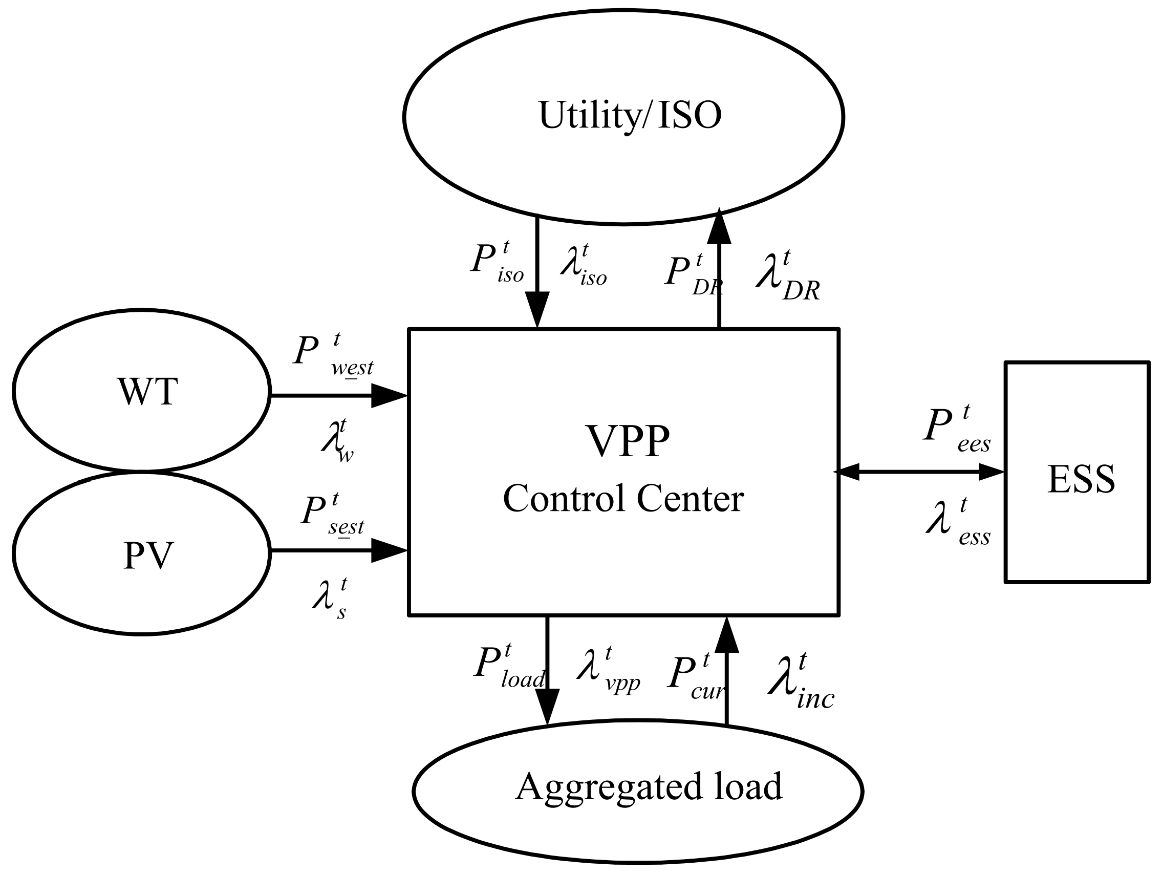
2. Problem Formulation

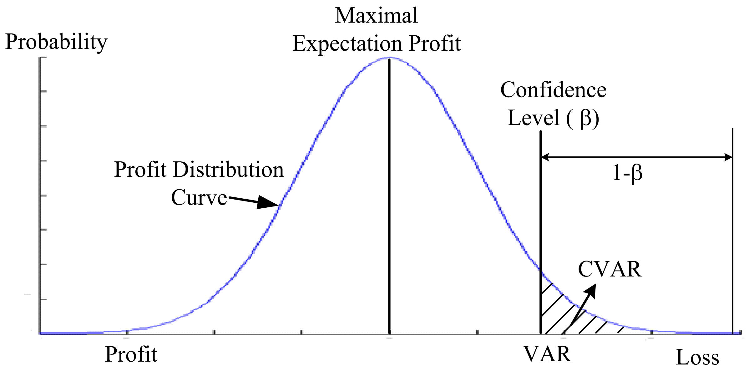
The VPP’s architecture studied in this paper is shown in Figure 1. The VPP control center has a link to the utilities/independent system operator (ISO), integrating wind power, solar power, and energy storage systems (ESS), and sells power to aggregated loads in order to obtain profit. The ISO selling power to the VPP determines whether or not to perform demand response (DR), which involves money rebate to the VPP. If DR is performed, the VPP will curtail the aggregated loads and return part of the rebate to the aggregated load. In the uncertain environment with wind and solar, VPPs seek to maximize the risk return of power dispatch through power trading and DR.

2.1. CVAR Model

Let $f(x,y)$ be a loss function with a set of decision variables $x$ and random variables $y$. $\rho (y)$ is a probability density function for VAR with $\beta$ confidence level and can be represented in Equation (1). By using the model in [28,29], we have

$${\mathrm{VAR}}_{\beta }(x)=\min \{\alpha \in R;{\displaystyle {\int }_{f(x,y)\le \alpha }\rho (y)dy\ge \beta \}}$$

(1)

CVAR, for a confidence level $\beta$, is defined as

$${\phi }_{\beta }(x)=E[f(x,y)|f(x,y)\ge {\mathrm{VAR}}_{\beta }(x)]=\frac{1}{1-\beta }{\displaystyle {\int }_{f(x,y)\ge VaR(x)}f(x,y)\rho (y)dy}$$

(2)

CVAR of the cost, calculated in NT$, can be approximated by

$$F_{\beta }(x,\mathrm{VAR})=\mathrm{VAR}+\frac{1}{1-\beta }{\displaystyle {\int }_{y\in R}[f(x,y)-\mathrm{VAR}]\rho (y)dy}$$

(3)

In Equation (3), CVAR can be expressed as a discrete function as in Equation (4).

$$F_{\beta }(x,\mathrm{VAR})=\mathrm{VAR}+\frac{1}{m(1-\beta )}{\displaystyle \sum _{k=1}^m[f(x,y^k)-\mathrm{VAR}}]$$

(4)

$F_{\beta }(x,\mathrm{VAR})$ is an estimated value of CVAR cost. $y^k$ are the k samples of variable $y$.

VAR is an estimate of loss for a given probability of occurrence. The given probability is called the confidence level, which represents the degree of the VAR. The VAR value is a threshold. We know the probability of future losses exceeding this threshold, but do not know how bad the situation is when the loss exceeds this threshold.

CVAR cost refers to the condition where loss exceeds the given VAR value. CVAR takes into account the characteristics of tail events, satisfaction of positive homogeneity, transmission immutability, and subadditivity. It can overcome several disadvantages of the VAR measure and become more accurate in risk assessment. The difference between VAR and CVAR is shown in Figure 2. VAR relates to the probability of loss excess and CVAR is the expectation of loss excess. CVAR is generally preferable, is more widely used, and is used in this paper.

2.2. The Power Output of the PVs/WTs

In this paper, an Excel database was constructed with data from the Central Weather Bureau Observation Data Inquiry System (CODIS) [30]. The least square support vector machine (LSSVM) [31] was developed for wind speed and global radiation forecasts, as shown in Figure 3. The LSSVM performs model training, where data of the input layer are trained and transferred to the output layer using the radial basis function network (RBFN) with kernel function, $K{\left(x,y\right)}^{}=e^{\left(-{\sigma }^2{\left|x-y\right|}^2\right)}$. The function can yield a good prediction, while error is calculated by using mean absolute percentage error (MAPE) as

$$\mathrm{MAPE}=\frac{1}{T}{\displaystyle \sum }_{t=1}^T\frac{\left|S_t^A-S_t^F\right|}{S_t^A}\times 100\%$$

(5)

where $S_t^A$ is the ‘time $t$ actual data’ to be forecast, while $S_t^F$ is the ‘time $t$ data’ constructed with LSSVM. $T$ is training time.

By using the predicted value of solar radiation and wind speed, power generation of PV and WT is simultaneously calculated as

$$P_{w\_est}^t=\frac{1}{2}\hspace{0.17em}\rho \hspace{0.17em}\hspace{0.17em}{C}_p(\lambda ,\theta )\hspace{0.17em}A{v}_t^3$$

(6)

$$P_{s\_est}^t={\eta }_{PV}\times P_G^t\times A_{PV}$$

(7)

$C_p(\lambda ,\theta )$ is assigned as follows.

$$C_p(\lambda ,\theta )=0.73\times ((\frac{151}{{\lambda }_i}-0.58\theta -0.002{\theta }^{2.14}-13.2)\times e^{-\frac{18.4}{{\lambda }_i}})$$

(8)

$${\lambda }_i=\frac{1}{\hspace{0.33em}\frac{1}{\lambda -0.02\theta }\hspace{0.33em}\hspace{0.33em}-\hspace{0.33em}\hspace{0.33em}\frac{0.003}{{\theta }^3+1}\hspace{0.33em}}$$

The ON/OFF status of the WT is explained in Equation (9).

$$\left\{\begin{array}{l}{v}_t=v_t^i\hspace{1em}\hspace{1em}\hspace{1em}\hspace{0.33em}\hspace{0.33em}\hspace{1em}if\hspace{1em}{v}_{start}\le v_t\le v_{full}\\ v_t=v_{full}\hspace{1em}\hspace{1em}\hspace{1em}\hspace{0.33em}\hspace{0.33em}if\hspace{1em}{v}_{full}<v_t<v_{stop}\\ v_t=0\hspace{1em}\hspace{1em}\hspace{1em}\hspace{1em}\hspace{0.33em}if\hspace{1em}{v}_{stop}\le v_t\hspace{1em}or\hspace{1em}{v}_t<v_{start}\end{array}\right.$$

(9)

2.3. The Model for the ESS

The power output of ESS can be calculated as the difference between the stored energies of two consecutive stages. Regardless of charging or discharging, ESS must be traded with the VPP. ESS is expressed as follows [32]:

• If the battery is charging:

  $$-{\eta }_c{P}_{ess}^t\le k_c{Q}_{s,max}$$

  (10)

  $$Q_s^{t+1}=Q_s^t-{\eta }_C{P}_{ees}^t\mathsf{\Delta }t$$

  (11)
• If the battery is discharging:

  $$\frac{P_{ees}^t}{{\eta }_D}\le k_D{Q}_s^t$$

  (12)

  $$Q_s^{t+1}=Q_s^t-\frac{P_{ees}^t\mathsf{\Delta }t}{{\eta }_D}$$

  (13)

  where ${\eta }_C$ and ${\eta }_D$ are charging efficiency and the discharging efficiency, both are brand-dependent. $P_{ees}^t$ is the electrical power of the battery output at the $t-th$ h. $Q_s^t$ is the aggregated capacity of the batteries at $t-th$ h. $Q_{s,max}$ is the rated maximum storage energy. $k_c$/$k_D$ is the maximum portion of the rated capacity that can be added to/withdrawn from storage in an h. $\mathsf{\Delta }t$ is the scheduling hour. In this paper, $\mathsf{\Delta }t$ was equal to 1 h.

2.4. Objective Function and Constraints

The VPP needs to plot its daily dispatch in the electricity market, and the proposed model combines the expected profit and risk. The objective of Equation (14) is to maximize the VPP’s profit, where risk income is also included. Risk income equals the summation of the average income of the VPP under various scenarios, and the CVAR considers not only risk but also economic income. Total income and total cost of the VPP are formulated in Equations (15) and (16), respectively.

$${\mathit{Profit}}^{DA}=\mathit{Max}\left[\frac{1}{m}{\displaystyle \sum _{n=1}^m(R(n)-C(n))+}{\mu }^{DA}(\xi -\frac{1}{m(1-\beta )}{\displaystyle \sum _{n=1}^m{Z}_n\times R_{\exp }})\right]$$

(14)

$$R(n)={\displaystyle \sum _{t=1}^{k-1}{\lambda }_{vpp}^t\times }{\mathrm{P}}_{\mathit{load}}^{\mathrm{t}}+{\displaystyle \sum _{t=k}^l({\lambda }_{vpp}^t}(P_{load}^t-P_{cur}^t)+{\lambda }_{DR}^t{P}_{DR}^t)+{\displaystyle \sum _{t=l+1}^{24}{\lambda }_{vpp}^t{P}_{load}^t}$$

(15)

$$\begin{array}{l}C(n)={\displaystyle \sum _{t=1}^{k-1}({\lambda }_{iso}^t}{\mathrm{P}}_{\mathrm{iso}}^{\mathrm{t}}\pm {\lambda }_{ess}^t{P}_{ess}^t+{\lambda }_w^t{P}_{w\_est}^t+{\lambda }_s^t{P}_{s\_est}^t)+{\displaystyle \sum _{t=k}^l({\lambda }_{inc}^t{P}_{cur}^t}+{\lambda }_{iso}^t{\mathrm{P}}_{\mathrm{iso}}^{\mathrm{t}}\pm {\lambda }_{ess}^t{P}_{ess}^t+{\lambda }_w^t{P}_{w\_est}^t+{\lambda }_s^t{P}_{s\_est}^t)\\ \hspace{1em}\hspace{1em}\hspace{1em}+{\displaystyle \sum _{t=l+1}^{24}({\lambda }_{iso}^t{\mathrm{P}}_{\mathrm{iso}}^{\mathrm{t}}\pm {\lambda }_{ess}^t{P}_{ess}^t+{\lambda }_w^t{P}_{w\_est}^t+{\lambda }_s^t{P}_{s\_est}^t})\end{array}$$

(16)

The daily dispatch in the objective function is divided in three intervals. DR interval is performed from h $k\text{-}th$ to h $l\text{-}th$. During the NO_DR interval, the profit of the VPP only comes from selling the electricity to the aggregated load, while the costs of the VPP will include the cost of buying electricity from ISO, WTs, PVs, and the operating cost of the battery. The profit of the DR interval includes the profit of selling electricity after load curtailment (${\lambda }_{vpp}^t(P_{load}^t-P_{cur}^t)$) and the provision of ISO to rebate any money (${\lambda }_{DR}^t{P}_{DR}^t$) to DR. Similarly, the VPP must provide the rebate money to the aggregated load in the DR interval (${\lambda }_{inc}^t{P}_{cur}^t$).

The following constraints are also defined with:

(1)

VPP energy balance constraint

$$P_{load}^t=P_{iso}^t+P_{ess}^t+P_{cur}^t+P_{w\_est}^t+P_{s\_est}^t$$

(17)

(2)

demand response

$$P_{cur}^t=P_{load}^t\times (1-e^{-{\theta }^t({\lambda }_{{}_{inc}}^t-{\lambda }_{vpp}^t)})$$

(18)

(3)

rebate constraints

$${\lambda }_{vpp}^t\le {\lambda }_{inc}^t\le {\lambda }_{DR}^t$$

(19)

(4)

the expected return on investment

$$\zeta -(R(n)-C(n))\le Z_n\times R_{\exp }$$

(20)

(5)

the rate of expected return on investment

$$Z_n=\frac{R(n)-C(n)}{C(n)}\ge 0$$

(21)

(6)

the capacity of battery

$$0\le \left(P_{ees}^{initial}+{\displaystyle \sum _{t=1}^H{P}_{ees}^t}\right)\le P_{ees,\mathit{max}}$$

(22)

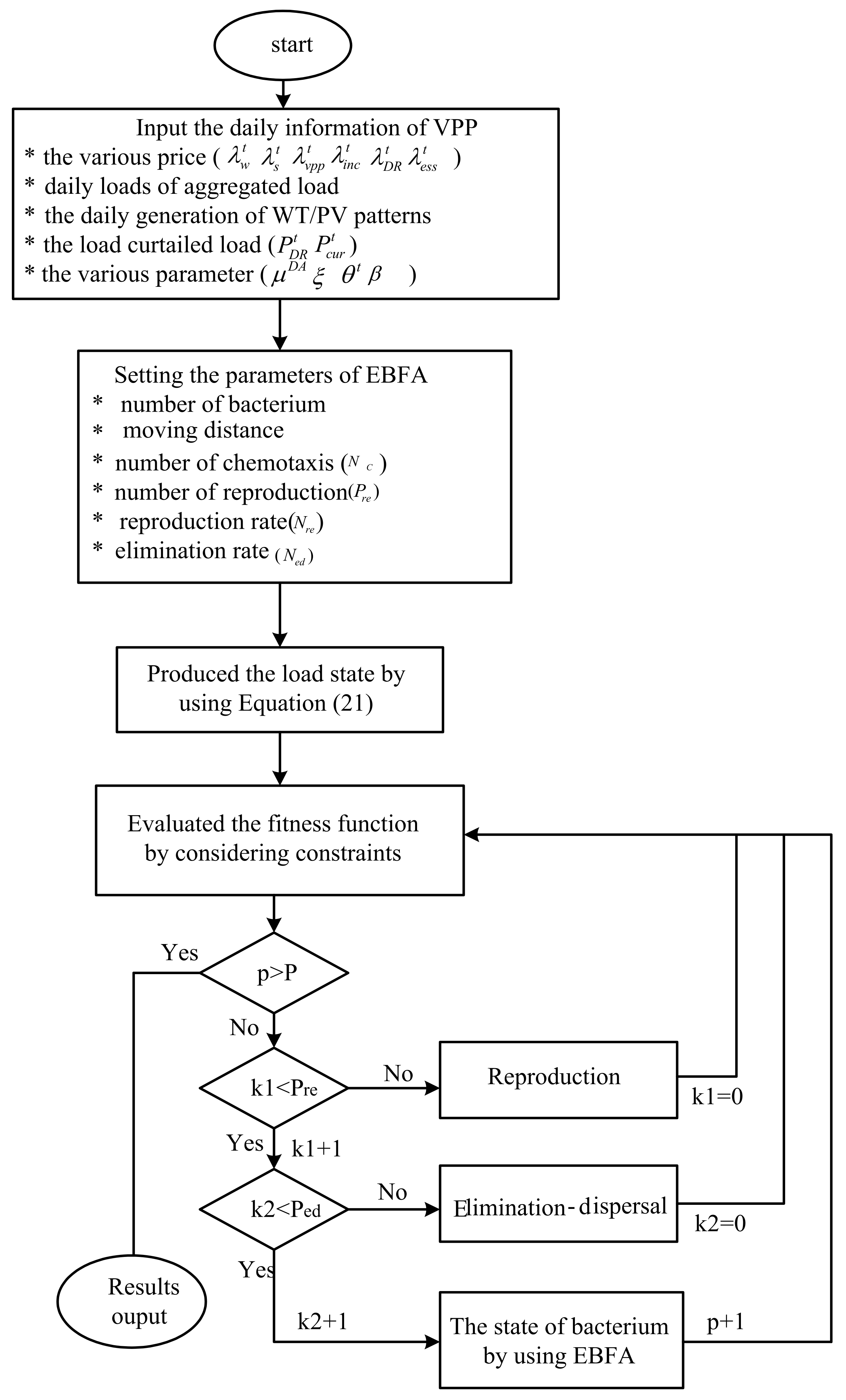
3. Solution Algorithm

In 2002, ref. [33] proposed a bacterial foraging algorithm (BFA) for numerical analysis. BFA produces a set of initial solutions, known as E. coli, and then looks for the optimal value through chemotaxis, reproduction, and elimination–dispersal. Bacteria must constantly move the position of individuals in the process of evolution, and gradually move to a better environment. For efficient performance, BFA is modified by hybrid stochastic weight trade-off [34] in this paper and is called EBFA. EBFA was developed as follows.

3.1. Bacterial Chemotaxis

The bacterial chemotaxis can be described as

$${\theta }^i(j+1,k,l)={\theta }^i(j,k,l)+C(i)\phi (j)$$

(23)

where ${\theta }^i(j,k,l)$ is the location of the $i\text{-}th$ bacterium at the $j\text{-}th$ chemotactic step, $k\text{-}th$ is the reproduction step, and $l\text{-}th$ is the elimination–dispersal event. $C(i)$ is the distance of the bacterium at each step and $\phi (j)$ is the tumble direction of the bacterium. Let $J(i,j,k,l)$ be defined as the fitness value of the $i\text{-}th$ bacterium. If the fitness $J(i,j+1,k,l)$ of ${\theta }^i(j+1,k,l)$ is lower than the fitness $J(i,j,k,l)$ of ${\theta }^i(j,k,l)$, $C(i)$ will remain in the same direction. Conversely, $\phi (j)$ will turn in another direction. Bacterial chemotaxis depends on the moving distance ($C(i)$) and the tumble direction ($\phi (j)$). If the useful chemotaxis message is not transmitted among the bacteria, it will lead to a local minimum. In order to improve the local searching capability, a stochastic weight trade-off is integrated in EBFA. The bacterial chemotaxis is modified by using Equation (24) as

$${\theta }^i(j+1,k,l)={\theta }^i(j,k,l)+C{(i)}^{\prime }\times {\xi }_j{r}_{1}Sign(r_2)\phi (j)$$

(24)

$r_1,r_2$: random number between 0 and 1;

$Sign$: freak factor.

$$Sign(r_2)=\left\{\begin{array}{l}1\hspace{1em}\hspace{0.33em}\hspace{0.33em}{r}_2>P_{let}\\ -1\hspace{1em}{r}_2\le P_{let}\end{array}\right.$$

(25)

$P_{let}$: the probability of “lethargy”.

$C{(i)}^{\prime }$ is the distance factors, varying according to the stage of optimal process [35] as

$$C{(i)}^{\prime }=(C_{max}^{}-C_{min}^{})\frac{S}{S_{max}}+C_{min}^{}$$

(26)

${\xi }_j$ is a control parameter, which is used to reduce the stochastic effect linearly. ${\xi }_j$ varies with the stage of optimal process:

$${\xi }_j=({\xi }_{min}-{\xi }_{max})\frac{S}{S_{max}}+{\xi }_{max}$$

(27)

The values of maximum iterations, ${\xi }_{\mathit{min}}$, ${\xi }_{\mathit{max}}$ and $P_{let}$ are set to 0.5, 2.5, and 0.5, respectively.

3.2. Bacterial Reproduction

Optimization is performed based on the fitness value $J(i,j,k,l)$. For the chemotaxis step, the fitness value is calculated with Equation (28) as

$$J_{health}^i={\displaystyle \sum _{j=1}^{N_C+1}J(i,j,k,l)}$$

(28)

$N_C$: the maximum step in the chemotaxis step.

In the reproduction process, the bacteria are sorted in ascending order by fitness and the better half of the bacteria will split into two bacteria, placed at the same location. Constant population size was used for convenient coding.

3.3. Elimination–Dispersal

The elimination–dispersal of the bacteria is set by the number of chemotaxis ($N_C$). After a new reproduction process, the new bacteria were dispersed from their original location according to the elimination–dispersal rate ($N_{ed}$) and moved to the best position within the searching space. The elimination–dispersal process will help to avoid premature convergence and entrapment in the local optimum.

Figure 4 is the flowchart of the applied EBFA.

4. Simulation Results

The proposed algorithm was simulated on a modified Penghu grid with renewables, as shown in Figure 5. The configuration of the VPP system consists of two WT fields, one PV fields, one thermal turbine, and one energy storage system (EES). The associated data for the study system are listed in

Table 1. The associated data of the modified Penghu grid system.

Unit	Number of Units	Capacity/Unit (MW)	Total Capacity (MW)
Wind turbine	8	0.6	4.8
Wind turbine	6	0.9	5.4
Solar power	1	12.9	12.9
Thermal turbine	1	129.8	129.8
EES	1	30	30

. Note that utility is represented by the real thermal units of Penghu island, capable of providing 129.8 MW power. In general, utility is transparent to the VPP, which needs the data of power output only, while the utility may have to deal with many VPPs. Table 1 is also modified by adding “utility” besides thermal. The load profile of a typical summer and non-summer day is shown in Figure 6, for example. Solving the risk dispatch problem of a VPP, hour-driven results are assumed in this paper, which could be extended to cover a different timespan or to become a daily operation. Summer and non-summer seasons refer to the two charge rates enforced by the Tai-Power Company in Taiwan [36]. Many scenarios were tested and analyzed. Two typical scenarios are shown as examples.

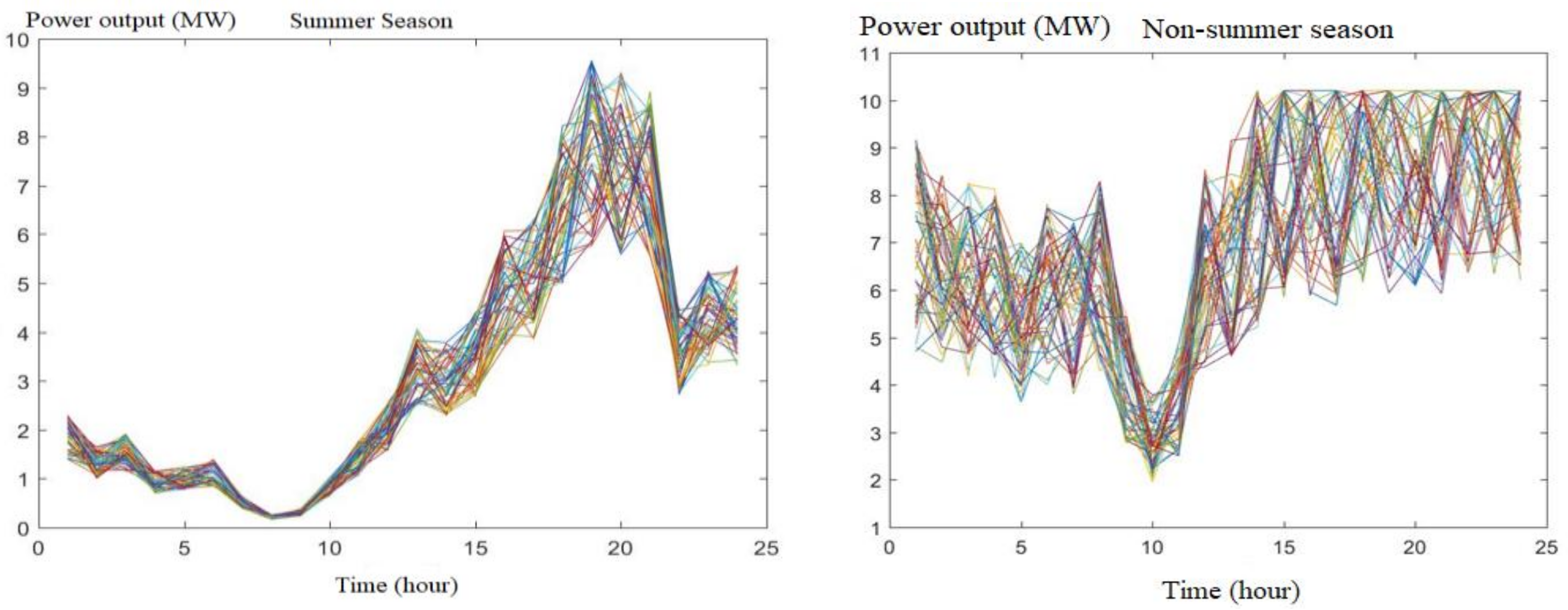
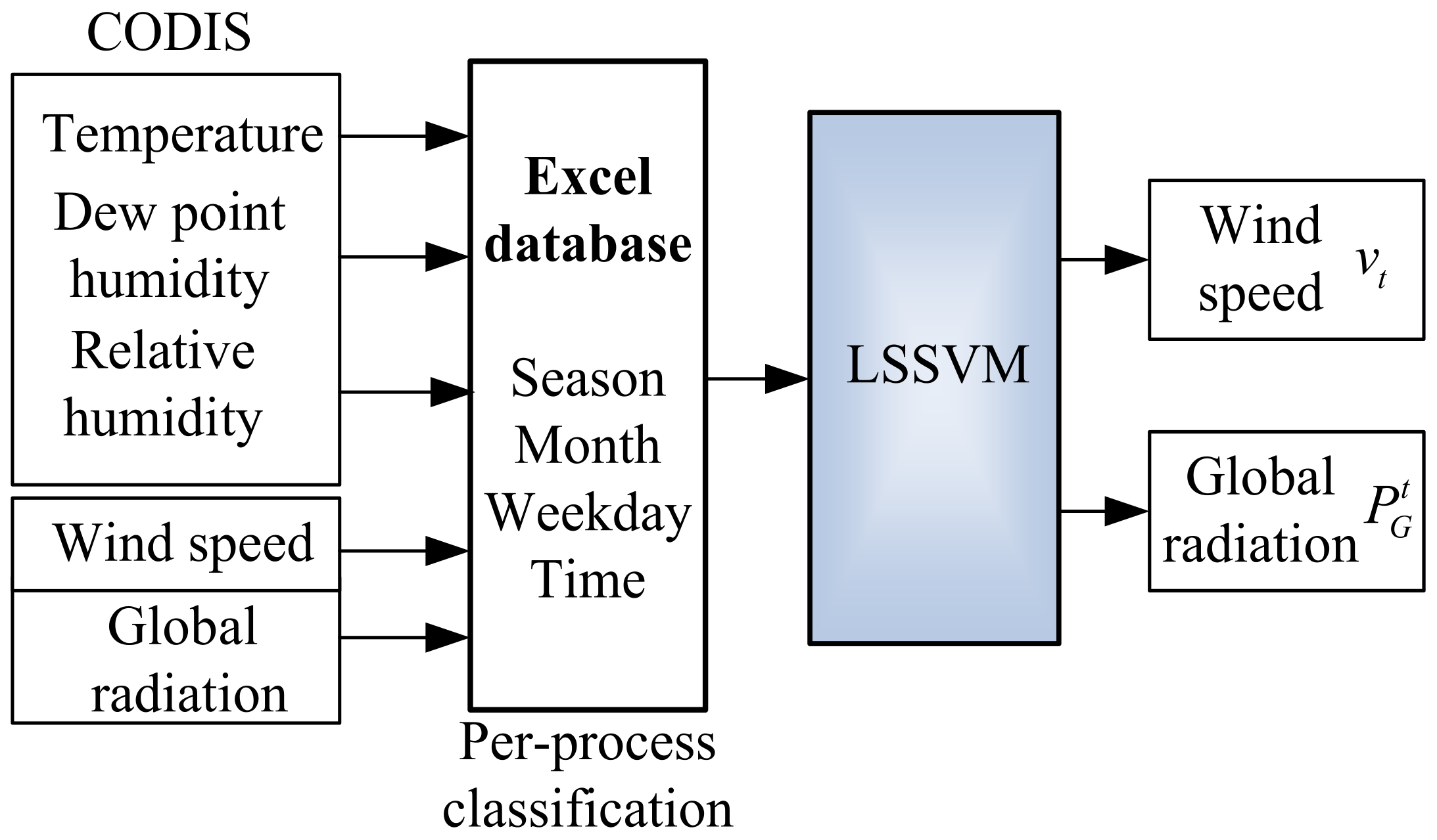
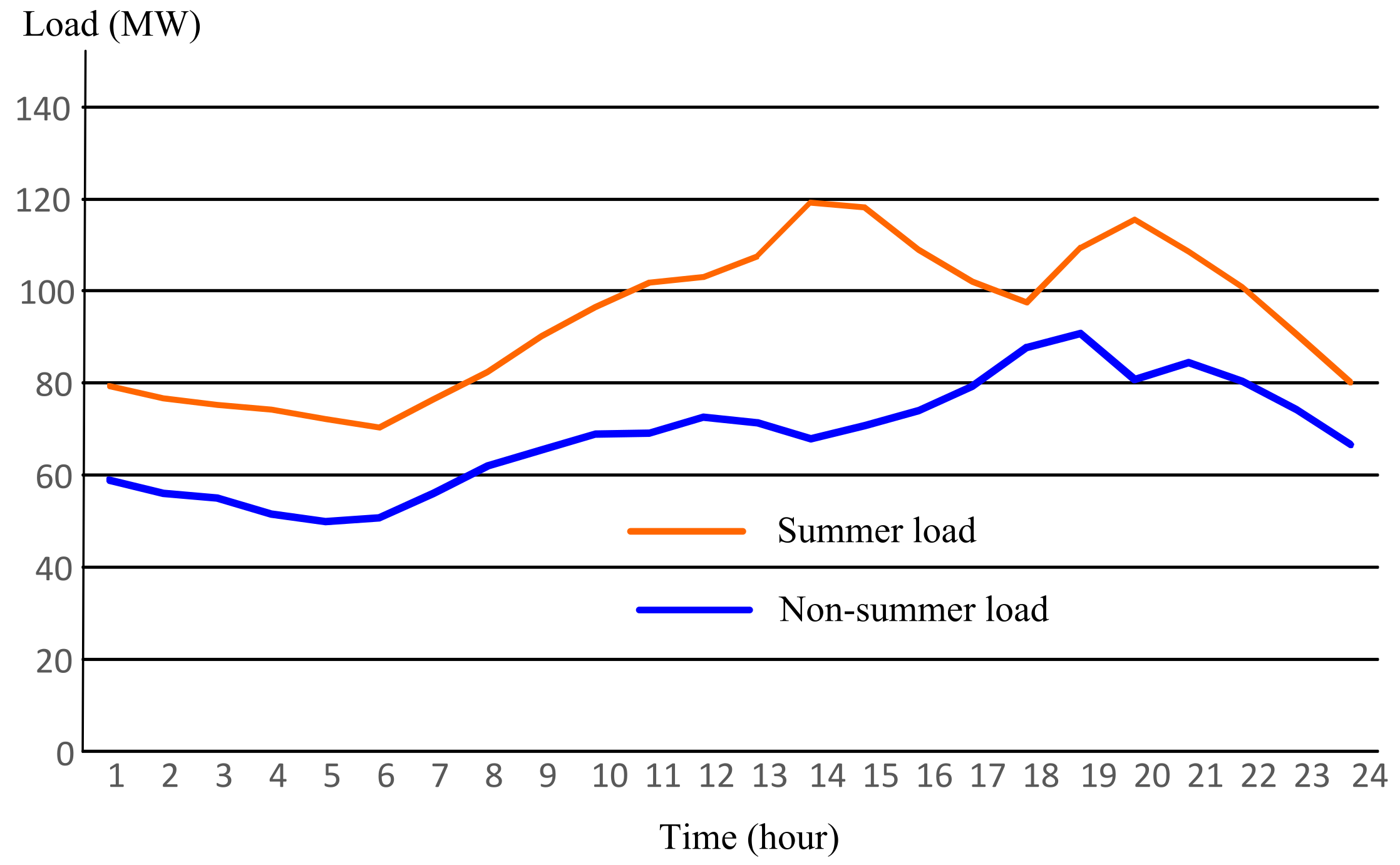
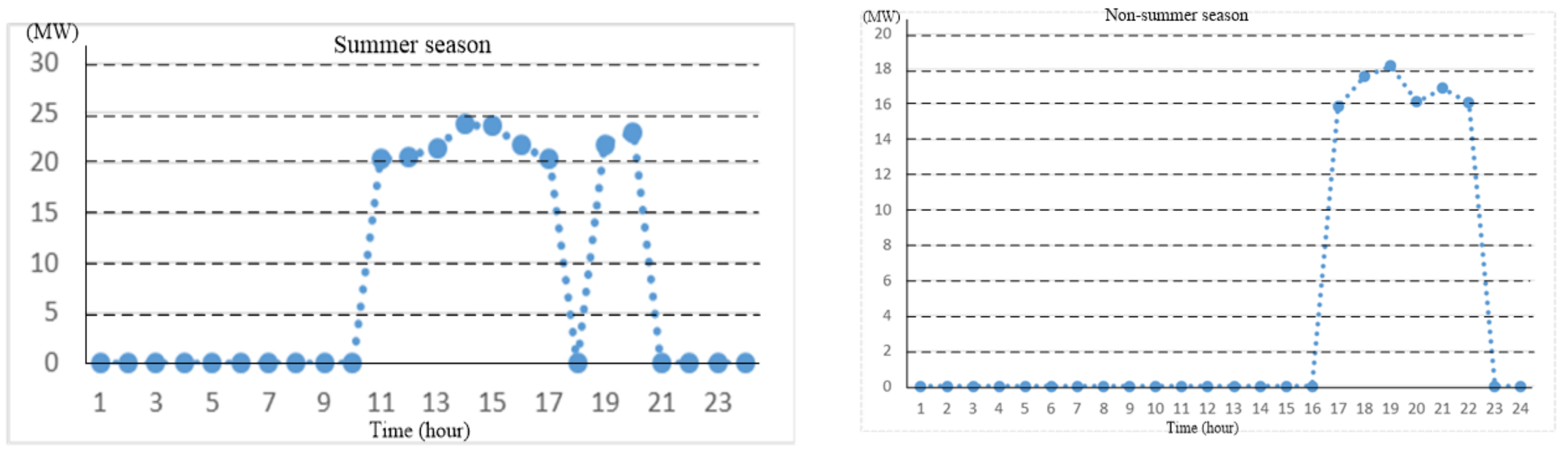
4.1. The Power Output of the PVs/WTs in the Summer/Non-Summer

The weather data used are from 1 July 2018 to 21 July 2018 and 1 December 2018 to 31 December 2018. The time horizon chosen was one day of 24 h. By using LSSVM, the wind speed and global radiation were forecast simultaneously, where the power output of WT/PV was calculated using Equations (6) and (7). The number of data samples for CVAR was 50. The emulation results of WT/PV power output are shown in Figure 7 and Figure 8. Figure 7 shows the power output of PV in the summer and non-summer seasons, and Figure 8 shows the power output of WT in the summer and non-summer seasons.

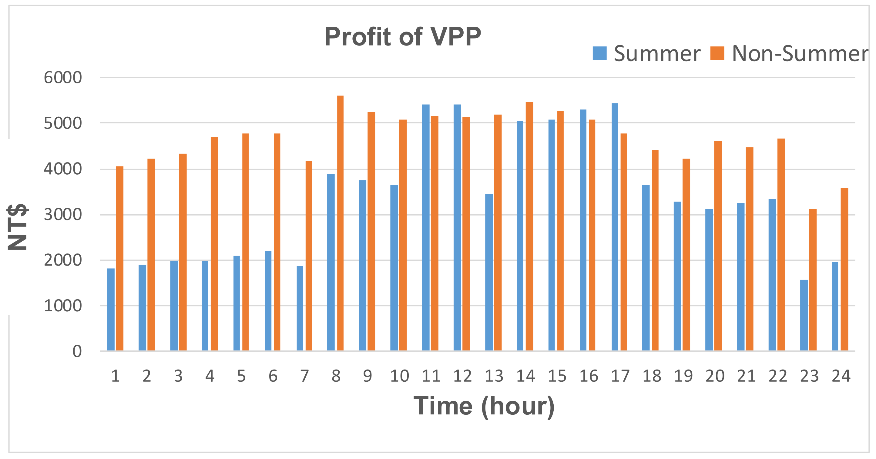
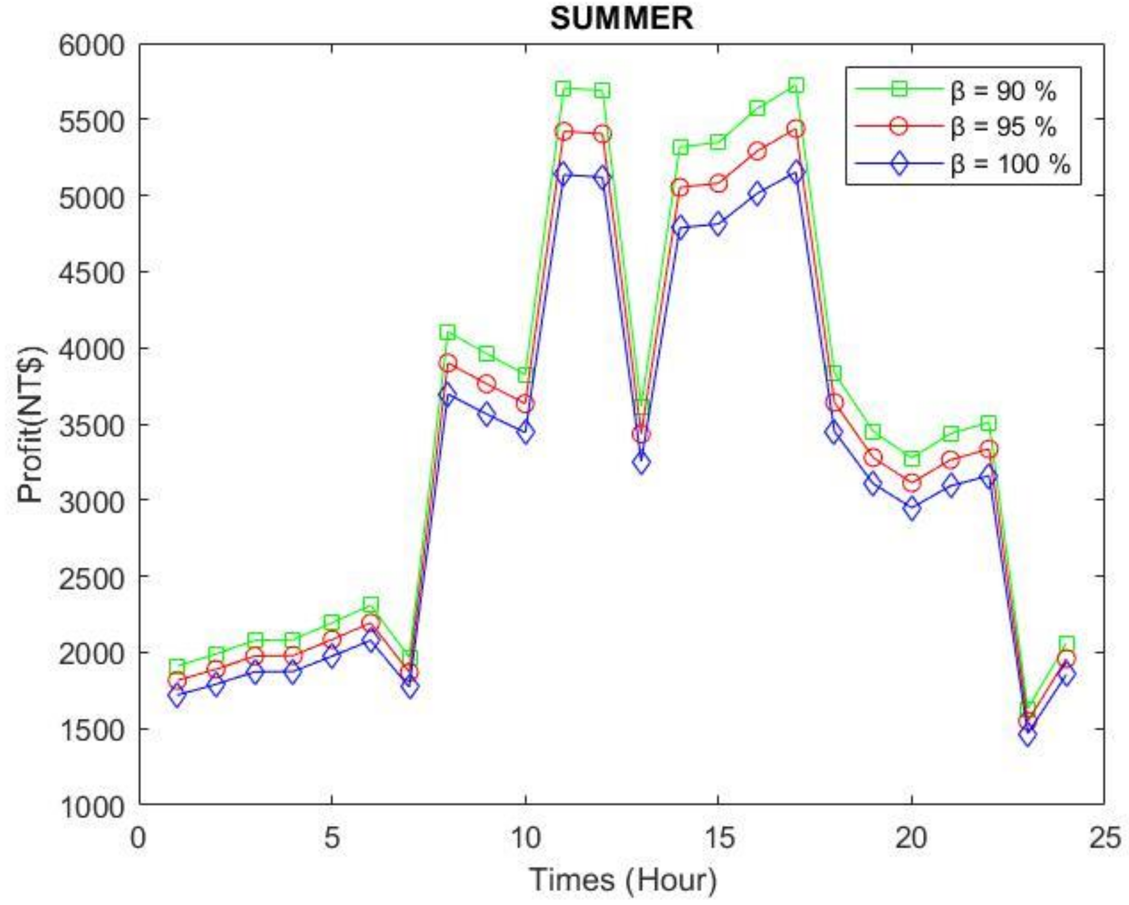
4.2. Results from Various Scenarios

To analyze the performance of VPPs, the number of data samples, risk level, and aversion parameter are 50, 95%, and 0.4, respectively. The cost–benefit power trading between VPP and utility needs to meet aggregated loads. Figure 9 shows the daily profit of the VPP for the summer and non-summer seasons with renewable uncertainties. Since the peak load usually occurs in the summer, the control center of the VPP must pay more rebate to aggregated loads for performing the DR.

Table 2. The total income and total cost of the VPP in the daily dispatch.

	Summer Season		Non-Summer Season
	Without DR	With DR	Without DR	With DR
Total income (NT$)	15,053,126	15,745,634	14,594,450	14,550,596
Total cost (NT$)	7,134,183	7,462,386	6,916,801	6,896,017
Profit (NT$)	7,918,943	8,283,248	7,677,649	7,654,579

shows the total income and total cost of the VPP in the daily dispatch. Table 2 shows that the dispatch with DR can gain more profit in the summer, but not the non-summer period.

Figure 10 shows the load curtailment in the summer and non-summer seasons. On a summer day, the control center of the VPP must curtail more load to satisfy the objectives. On the contrary, the VPP needs to curtail less of the load to obtain a better profit in the non-summer season.

Figure 11 shows the CVAR and the summer daily profit of the VPP with various confidence levels ($\beta$ = 100%, $\beta$ = 95%, $\beta$ = 90%). The CVAR in Figure 11 shows that a higher confidence level leads to a lower CVAR of maximal profit, i.e., with a lower risk.

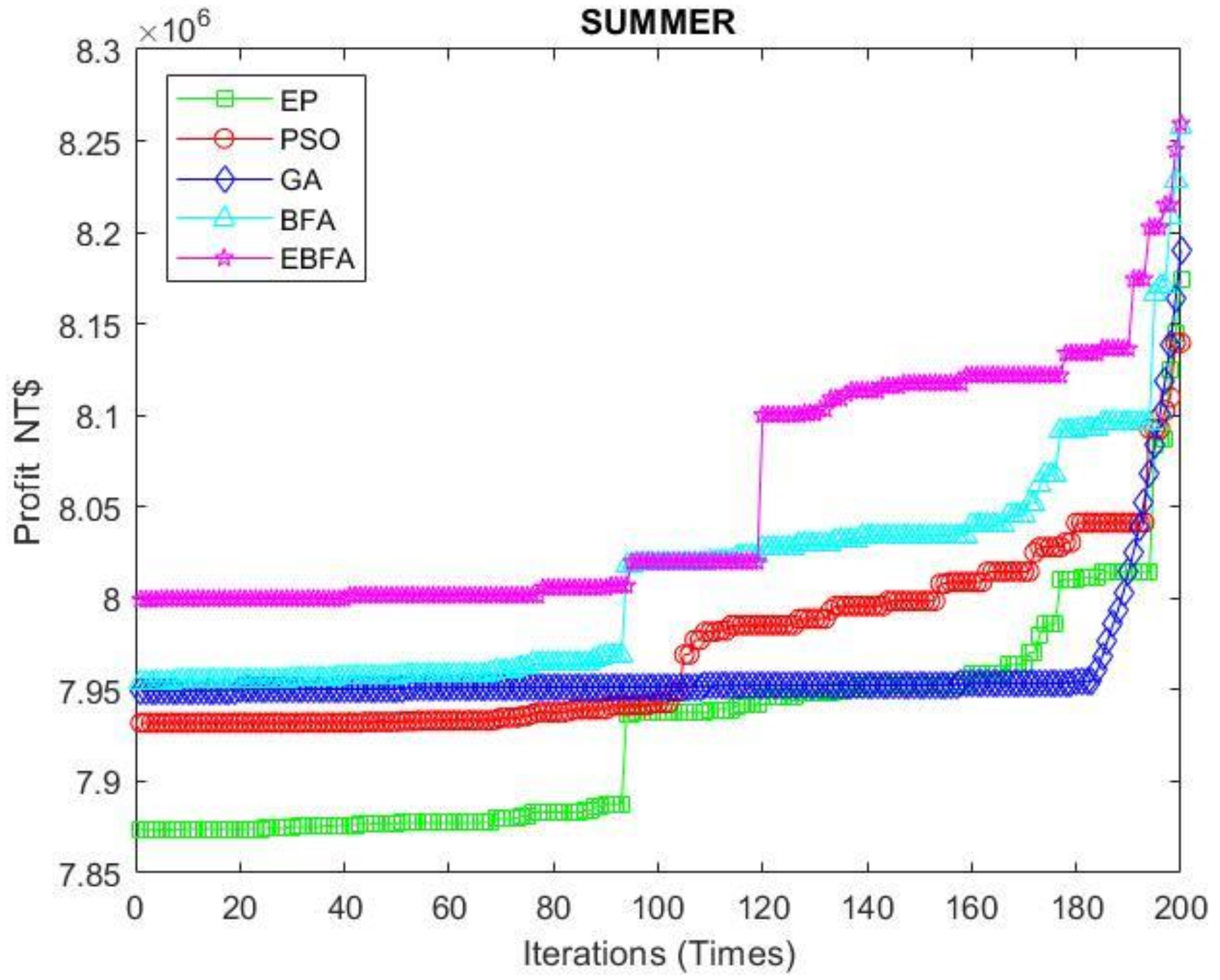
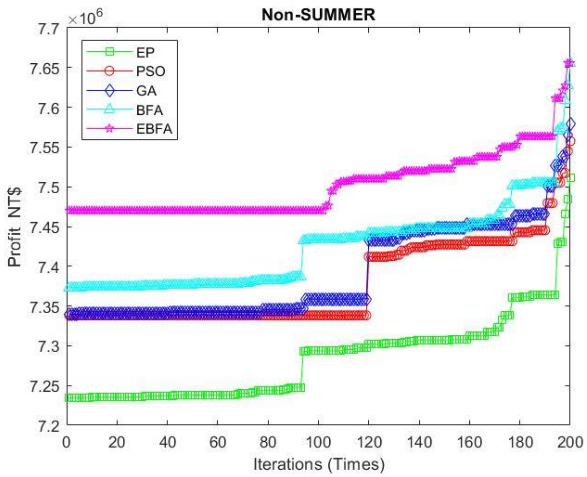
4.3. Convergence Test

Table 3. Robustness test for EP, GA, PSO, BFA, and EBFA algorithms.

	Summer		Non-Summer
Algorithm	Maximal Converged Profit (NT$)	Average Execution Times (s)	Maximal Converged Profit (NT$)	Average Execution Times (s)
EP	8,174,430	238	7,623,943	245
PSO	8,139,733	227	7,639,699	234
GA	8,190,471	237	7,639,155	244
BFA	8,259,395	213	7,654,015	219
EBFA	8,283,248	227	7,654,580	234

shows a comparison chart of using evolutionary programming (EP), genetic algorithm (GA), particle swarm optimization (PSO), BFA, and EBFA in the simulation. The tests were performed using an Intel Core i7-6700HQ, 3.4 Hz CPU with 8 GB DRAM. Each algorithm was tested 100 times with the same initial values. It can be seen that EBFA improves the searching efficiency with the best probability of guaranteeing a global optimum. Table 3 shows that EBFA can maximize the profit better than EP, GA, PSO, and BFA, i.e., it yields the greatest profit among all the methods, with the average execution time only a little longer than BFA. Figure 12 and Figure 13 show the convergent characteristics of EP, GA, PSO, BFA, and EBFA for the summer and non-summer periods. They also show that EBFA has a better capability to explore a better global optimum.

5. Conclusions

This paper developed an EBFA algorithm to solve the risk dispatch of a VPP to obtain maximal profit. By considering WTs and PVs, uncertainties of load and VAR of power generation were integrated into the searching process. EBFA can solve the complicated problem with a better efficiency than other algorithms and can obtain a global optimum. It has great potential to be further applied to many non-convex problems in power system planning and operation. The EBFA successfully demonstrated its performance on the Penghu VPP system. By considering various scenarios, the maximal risk and return of the VPP were simulated and analyzed. Results show a good opportunity for VPPs to perform power dispatch by maximizing risk income. The proposed algorithm can be integrated into real-time operations and applied to many other mixed integer combinational optimization problems for power systems.

References

1. Jiayi, H.; Chuanwen, J.; Rong, X. A review on distributed energy resources and Microgrid. Renew. Sustain. Energy Rev. 2008, 12, 2472–2483. [Google Scholar] [CrossRef]
2. Liu, C.; Yang, R.J.; Yu, X.; Sun, C.; Wong, S.P.; Zhao, H. Virtual power plants for a sustainable urban future. Sustain. Cities Soc. 2021, 65, 102640. [Google Scholar] [CrossRef]
3. Yu, S.; Fang, F.; Liu, Y.; Liu, J. Uncertainties of virtual power plant: Problems and countermeasures. Appl. Energy 2019, 239, 454–470. [Google Scholar] [CrossRef]
4. Dabbagh, S.; KazemSheikh-El-Eslami, M. A profit sharing scheme for distributed energy resources integrated into a virtual power plant. Appl. Energy 2016, 184, 313–328. [Google Scholar] [CrossRef]
5. Shafiekhani, M.; Badri, A.; Khah, M.; Catalao, J. Strategy bidding of virtual power plant in energy markets: A bi-level multi-objective approach. Int. J. Electr. Power Energy Syst. 2019, 113, 208–219. [Google Scholar] [CrossRef]
6. Kardakos, E.G.; Simoglou, C.K.; Bakirtzis, A.G. Optimal Offering Strategy of a Virtual Power Plant: A Stochastic Bi-Level Approach. IEEE Trans. Smart Grid 2016, 7, 794–806. [Google Scholar] [CrossRef]
7. Hu, H.; Jiang, C.; Liu, Y. Short-term bidding strategy for a price-maker virtual power plant based on interval optimization. Energies 2019, 32, 3662. [Google Scholar] [CrossRef] [Green Version]
8. Sun, B.; Kong, X.; Yang, Q. Demand-responsive virtual power plant optimization scheduling method based on competitive bidding equilibrium. Energy Procedia 2019, 158, 3988–3993. [Google Scholar] [CrossRef]
9. Nosratabadi, S.; Hooshmand, R.; Gholipour, E. A comprehensive review on microgrid and virtual power plant concepts employed for distributed energy resources scheduling in power systems. Renew. Sustain. Energy Rev. 2017, 67, 341–363. [Google Scholar] [CrossRef]
10. Maanavi, M.; Najafi, A.; Godina, R.; Mahmoudian, M.; Rodrigues, E. Energy Management of Virtual Power Plant Considering Distributed Generation Sizing and Pricing. Appl. Sci. 2019, 9, 2817. [Google Scholar] [CrossRef] [Green Version]
11. Duan, J.; Wang, X.; Gao, Y.; Yang, Y.; Yang, W.; Li, H.; Ehsan, A. Multi-Objective Virtual Power Plant Construction Model Based on Decision Area Division. Appl. Sci. 2018, 8, 1484. [Google Scholar] [CrossRef] [Green Version]
12. Wu, H.; Liu, X.; Ye, B.; Xu, B. Optimal dispatch and bidding strategy of a virtual power plant based on a Stackelberg game. IET Gener. Transm. Distrib. 2020, 14, 552–563. [Google Scholar] [CrossRef]
13. Tang, W.; Yang, H.T. Optimal operation and bidding strategy of a virtual power plant integrated with energy storage systems and elasticity demand response. IEEE Access 2019, 7, 79798–79809. [Google Scholar] [CrossRef]
14. Nguyen, H.T.; Le, L.B.; Wang, Z. A bidding strategy for virtual power plants with the intraday demand response exchange market using the stochastic programming. IEEE Trans. Ind. Appl. 2018, 54, 3044–3055. [Google Scholar] [CrossRef]
15. Sun, G.; Qian, W.; Huang, W.; Xu, Z.; Fu, Z.; Wei, Z.; Chen, S. Stochastic Adaptive Robust Dispatch for Virtual Power Plants Using the Binding Scenario Identification Approach. Energies 2019, 12, 1918. [Google Scholar] [CrossRef] [Green Version]
16. Ko, R.; Kang, D.; Joo, S. Mixed integer quadratic programming based scheduling methods for day-ahead bidding and intrs-day operation of virtual power plant. Energies 2019, 12, 1410. [Google Scholar] [CrossRef] [Green Version]
17. Zhang, J.; Xu, Z.; Xu, W.; Zhu, F.; Lyu, X.; Fu, M. Bi-Objective Dispatch of Multi-Energy Virtual Power Plant: Deep-Learning-Based Prediction and Particle Swarm Optimization. Appl. Sci. 2019, 9, 292. [Google Scholar] [CrossRef] [Green Version]
18. Meng, C.; Qin, P.; Wang, Y.; An, X.; Jiang, H.; Liang, Y. A revenue-risk equilibrium model for distributed energy integrated virtual power plants considering uncertainties of wind and photovoltaic power. In Proceedings of the 5th Asia Conference on Power and Electrical Engineering (ACPEE), Chengdu, China, 4–7 June 2020; pp. 2032–2038. [Google Scholar]
19. Dabbagh, S.R.; Sheikh-El-Eslami, M.K. Risk Assessment of Virtual Power Plants Offering in Energy and Reserve Markets. IEEE Trans. Power Syst. 2016, 31, 3572–3582. [Google Scholar] [CrossRef]
20. Alahyan, A.; Ehsan, M.; Pozo, D.; Farrokhifar, M. Hybrid uncertainty-based offering strategy for virtual power plants. IET Renew. Power Gener. 2020, 14, 2359–2366. [Google Scholar]
21. Castillo, A.; Flicker, J.; Hansen, C.; Waston, J.; Jhonson, J. Stochastic optimisation with risk aversion for virtual power plant operations: A rolling horizon control. IET Gener. Transm. Distrib. 2019, 13, 2063–2076. [Google Scholar] [CrossRef]
22. Liang, Z.; Alsafasfeh, Q.; Jin, T.; Pourbabak, H.; Su, W. Risk-Constrained Optimal Energy Management for Virtual Power Plants Considering Correlated Demand Response. IEEE Trans. Smart Grid 2019, 10, 1577–1587. [Google Scholar] [CrossRef]
23. Dahraie, M.; Kermani, A.; Moghaddam, A.; Siano, P. Risk-averse probabilistic framework for scheduling of virtual power plants considering demand response and uncertainties. Int. J. Electr. Power Energy Syst. 2020, 121, 106126. [Google Scholar] [CrossRef]
24. Kong, X.; Xiao, J.; Liu, D.; Wu, J.; Shen, Y. Robust stochastic optimal dispatching method of multi-energy virtual power plant considering multiple uncertainties. Appl. Energy 2020, 279, 115707. [Google Scholar] [CrossRef]
25. Gao, R.; Guo, H.; Zhang, R.; Mao, T.; Xu, Q.; Zhou, B.; Yang, P. A Two-Stage Dispatch Mechanism for Virtual Power Plant Utilizing the CVaR Theory in the Electricity Spot Market. Energies 2019, 12, 3402. [Google Scholar] [CrossRef] [Green Version]
26. Ju, L.; Tan, Q.; Lu, Y.; Tan, Z.; Zhang, Y.; Tan, Q. A CvaR-robust-based multi-objective optimization model and three stage solution algorithm for a vritual power plant considering uncertainties and carbon emission allowances. Int. J. Electr. Power Energy Syst. 2019, 107, 628–643. [Google Scholar] [CrossRef]
27. Lima, R.; Conejo, A.; Langodan, S.; Hoteit, I. Risk-averse formulations and methods for a virtual power plant. Comput. Oper. Res. 2018, 96, 349–372. [Google Scholar] [CrossRef]
28. Alexander, C. Risk Management and Analysis—Volume 1 Measuring and Modeling Financial Risk; John Wiley & Sons Ltd.: London, UK, 2000. [Google Scholar]
29. Marrison, C. Fundamentals of Risk Measurement; McGraw-Hill Companies, Inc.: New York, NY, USA, 2002. [Google Scholar]
30. Available online: https://www.cwb.gov.tw/V7/observe/real/46744.htm (accessed on 15 December 2020).
31. Suykens, J.A.K.; Vandewalle, J. Least square support vector machine. Neural Process. Lett. 1999, 9, 293–300. [Google Scholar] [CrossRef]
32. Lin, W.M.; Tu, C.S.; Tsai, M.T. Energy Management Strategy of the Microgrids by using Enhanced Bee Colony Optimization. Energies 2016, 9, 5. [Google Scholar] [CrossRef] [Green Version]
33. Passion, K.M. Biomimicry of bacterial foraging for distributed optimization and control. IEEE Control Syst. 2002, 22, 52–67. [Google Scholar]
34. Chalermchaiarbha, S.; Ongsakul, W. Stochastic weight trade-off particle swarm optimization for nonconvex economic dispatch. Energy Convers. Manag. 2013, 70, 66–75. [Google Scholar] [CrossRef]
35. Chaturvedi, K.T.; Pandit, M.; Srivastava, I. Self-organizing hierarchical particle swarm optimization for nonvex economic dispatch. IEEE Trans. Power Syst. 2008, 23, 1079–1087. [Google Scholar] [CrossRef]
36. TPC. Time-of-Use Rate for Users. The Electricity Rate Structure of Taipower Company; TPC: Taipei, Taiwan, 2020. [Google Scholar]
Figure 1. The VPP’s architecture.
Applsci 11 07752 g001
Figure 2. Diagram of the VAR and CVAR calculation.
Applsci 11 07752 g002
Figure 3. The wind speed/global radiation forecasting using the LSSVM.
Applsci 11 07752 g003
Figure 4. The flowchart of applied EBFA.
Applsci 11 07752 g004
Figure 5. The modified Penghu grid.
Applsci 11 07752 g005
Figure 6. Summer and non-summer load profile examples.
Applsci 11 07752 g006
Figure 7. The power output of PV in the summer and non-summer seasons.
Applsci 11 07752 g007
Figure 8. The power output of WT in the summer and non-summer seasons.
Applsci 11 07752 g008
Figure 9. The daily profit of the VPP in the summer and non-summer seasons.
Applsci 11 07752 g009
Figure 10. The daily load curtailment in the summer and non-summer seasons.
Applsci 11 07752 g010
Figure 11. The summer daily profit of the VPP with various confidence levels.
Applsci 11 07752 g011
Figure 12. The convergence characteristics of EP, GA, PSO, BFA, and EBFA in summer.
Applsci 11 07752 g012
Figure 13. The convergence characteristics of EP, GA, PSO, BFA, and EBFA in non-summer.
Applsci 11 07752 g013