Noninteracting Control Design for 6-DoF Active Vibration Isolation Table with LMI Approach

Abstract

This paper proposes a novel control strategy for six degrees-of-freedom active vibration isolation tables. In these systems, the most challenging issue is to suppress the external vibrations and isolate the internal interactions while still preserving the system’s robustness when facing uncertainties. A noninteracting controller is designed to tackle these problems. The resulting control system is completely decoupled in the sense that each system output is independently controlled to follow the corresponding reference signal. In this paper, the model of an active vibration isolation table is firstly derived. Conditions for system stability and decoupled performance are then discussed. The control law is formulated using the linear matrix inequality approach, which results in optimal control gains for the control objectives. With the proposed controller, complex system characteristics can be handled more efficiently such that an effective system is designed to obtain good control performance. Finally, simulations and comparison studies were conducted, and the results validate the efficiency of the proposed scheme.

1. Introduction

In recent years, the performance requirements of high-precision machinery and measuring instruments have increased at a rapid rate. Microscopes, 3D surface measurement systems, and nano analysis instruments can be named among them. These systems are very sensitive to ambient vibrations, such as ground vibration produced by other machines in the same workspace. A slight vibration may lead to undesirable system movements and the performance of the system deteriorates, which may result in product defects. Therefore, there is a need for mechanisms that isolate these systems from six degrees-of-freedom (DoF) vibrations on a wide range of frequencies. The vibration isolation capability determines the work performance in high-precision operations, which leads to a high level of manufacturing and measurement yields.

In general, there are two methods for vibration isolation: passive and active. The passive vibration isolation systems (PVIS), such as springs and dampers, are widely used for their low cost, simple installation, wide load range, and no external energy usage. The vibration isolation can be achieved with the appropriate dynamic structural design of a PVIS, such as in [1]. Although the PVIS can effectively suppress high-frequency vibrations, at low-frequency ranges, it is difficult to achieve satisfying vibration isolation performances. Moreover, the vibrations are amplified whenever their frequencies are near the system resonance frequency. In order to overcome the PVIS limitations, active actuators and advanced control techniques were introduced with the development of active vibration isolation systems (AVIS).

A typical vibration isolation system consists of two plates: a bottom plate fixed on the ground and a top plate carrying the machinery that needs isolating. Springs, dampers, and/or active actuators are situated between the two plates such that the weight of the machinery is supported, the vibration from the ground is suppressed, and the top plate is stabilized. Several types of actuators were used in AVIS systems; for instance, pneumatic actuators [2], hybrid actuators comprising pneumatic actuators and giant magneto-strictive actuators [3], piezoelectric stack actuators [4], and voice coil motors (VCMs) [5]. Each actuator has various advantages and disadvantages, as described in [6], which makes them suitable for diverse applications. VCMs, especially, are widely used because of their advantages, such as good linearity, low noise, and high acceleration and deceleration. In AVISs, the number of actuators must be equal to or greater than the controlled DoFs. Hence, vibrations in every direction can be suppressed; however, the resulting system is often over-actuated. Moreover, motion sensors, such as accelerometers, velocity sensors, and vibration sensors, are mounted directly to the top plate to sense the presence of movements of the machinery and a controller regulates the actuators accordingly. Additional sensors can also be mounted on the bottom plate and the ground vibration can be fed directly to the control systems. Moreover, there is little difference in the mechanical structure and the operating principle of vibration isolation systems. Therefore, recent studies have focused on the design of the control schemes rather than the system structure.

One of the greatest difficulties in controlling an AVIS is the large number of DoFs as well as the interactions between them. The presence of these interactions was clear in the system dynamics of the 6-DoFs model in [5] or even the simplified 2-DoFs suggested in [7]. Many authors have tried to propose control methods so that a controller for each DoF can be individually designed. For example, in [8], the author used the modal decomposition technique to transform the system model into a diagonal structure, and then proposed a proportional-integral-derivative (PID) to regulate the performance in each DoF. Vibration attenuation performance was presented, but only for one direction, whereas the response in other directions was not shown, hence, overall performance could not be concluded. In [5], the authors proposed a sheet current model that considers the end effects of the VCMs used in the design of a 6-DoF AVIS, and the parameters of the AVIS were identified using the hybrid functions approach. And then, a composite nonlinear feedback (CNF) controller was designed following the modal decomposition method. The CNF controller was designed for each pair of input–output, so there were six individual controllers in total. However, the identified model is incompatible with the dynamic characteristics and the interaction isolation performance of this control system was not discussed. Generally, the modal decomposition is well known to obtain the diagonal form of a system model, but it is a rather analytic method than a decoupling control approach. Another method treats the interactions as disturbances affecting the system. Kim et al. [7] proposed an $H_{\infty }$ control with a direct disturbance suppression technique and the effectiveness of the control strategy was verified using a 2-DoF AVIS. Unfortunately, this approach is only effective for the 2-DoF system and is difficult to implement for more complex systems.

Moreover, other decoupling techniques have been studied such that only one controller is designed for the whole system and all the interactions are effectively isolated. For instance, diagonal decoupling by static-state feedback [9], decoupling with dynamic compensation [10], noninteracting constraints [11], robust noninteracting control [12], input–output energy decoupling [13], row by row decoupling [14], and noninteracting control based on the relaxed control [15], as well as other decoupling controllers [16,17,18], have been applied in various applications. Nevertheless, the common issue with these control system designs lies in the analytical methodology of deriving the proper control matrices that not only decouple the interactions but also achieve the desired performance.

Therefore, in this paper, a new robust noninteracting control system design method for a 6-DoF AVIS system is proposed. The key point of the approach is that the resulting system configuration affects the control input in a way that each reference signal controls the corresponding control output without influencing the other ones. The proposed controller is designed based on an integral-type servosystem, which consists of state feedback and unity feedback. Conditions on the controller matrices are analyzed to obtain noninteracting performances. Even though the stability of the closed-loop system is not guaranteed, the system performance is not satisfied. Therefore, new methods to design the feedback-matrix gain and unity-feedback matrix gains are introduced. With the use of the linear matrix inequality (LMI) technique, the derived solutions provide optimal control matrices to fulfill both decoupling and stability requirements. The efficiency of the proposed control strategy was evaluated through two simulation scenarios: platform positioning and vibration isolation.

This paper is structured as follows: Section 2 presents the system modeling of the 6-DoF AVIS. In Section 3, the noninteracting control design is described in detail. Then, simulation results are presented in Section 4. Finally, the conclusions of this study are summarized in Section 5.

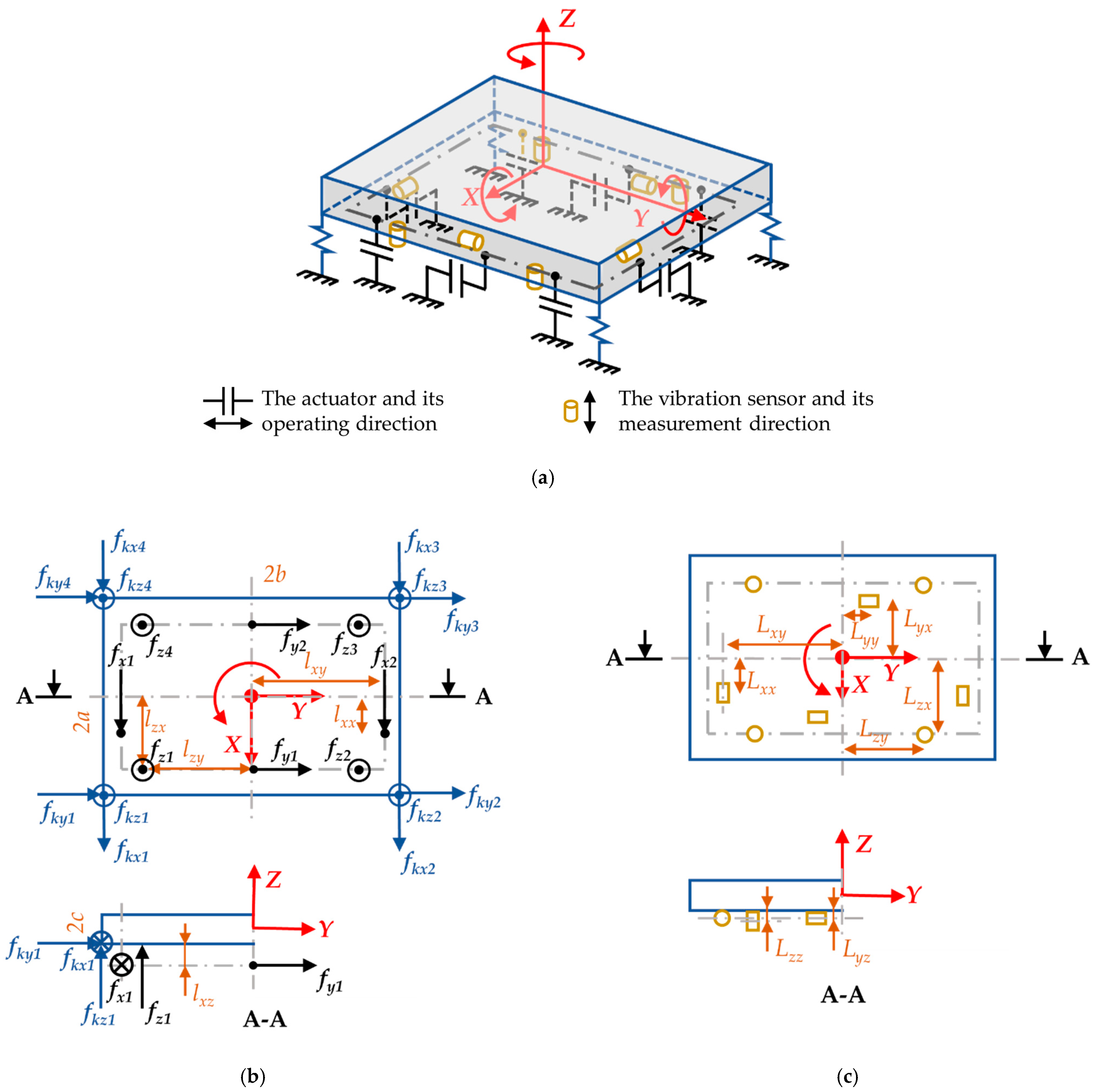
2. System Modeling

Figure 1 shows the schematic drawing of a 6-DoF AVIS and the allocation of the actuators and sensors is highlighted. The mechanical structure consists of a bottom plate fixed to the ground and a top plate carrying the machine that needs isolating from vibrations. There are four coil springs at the four corners connecting the two plates and supporting the mass of the top parts. To start with, let the coordinate systems be defined as follows:

• The top plate fixed frame T is a right-handed coordinate system whose origin is at the mass center of the plate; the Z-axis points upward, the X-axis points forward, the counterclockwise is the positive rotation direction. This coordinate system is depicted by red-colored vectors in Figure 1.
• The bottom plate fixed frame B has its origin at the centroid of the bottom plate. Translation and rotation directions are similar to frame T.

For the active isolation operation, eight VCMs generate linear forces between the two plates. Four of the VCMs generate translational movements perpendicular to the top plate, i.e., along the Z-axis. Two VCMs generate motions along the X-axis direction and the others along the Y-axis direction. Accordingly, eight vibration sensors have been arranged as shown in Figure 1.

Assumption 1: The top plate is geometrically symmetric, and its mass is uniformly distributed.

Assumption 2: Along an i-axis direction, each of the springs acts as a linear spring with the same stiffness $k_i$ and the same damping factor $c_i$.

For convenience’s sake, nomenclatures used in the remainder of the paper are listed as follows:

• $x={\left[\begin{array}{ccc}x& y& z\end{array}\right]}^T$ is the displacement of the origin O in the x-, y-, and z-directions;
• $\phi ={\left[\begin{array}{ccc}{\phi }_x& {\phi }_y& {\phi }_z\end{array}\right]}^T$ is the rotation about x-, y-, and z-axes of the upper plate;
• $x_b={\left[\begin{array}{ccc}{x}_b& y_b& z_b\end{array}\right]}^T$ and ${\phi }_b={\left[\begin{array}{ccc}{\phi }_x{}_b& {\phi }_y{}_b& {\phi }_z{}_b\end{array}\right]}^T$ are the displacement and the angular position of the bottom plate, respectively;
• m is the mass of the sprung weight;
• $J=\left[\begin{array}{ccc}{J}_{xx}& 0& 0\\ 0& J_{yy}& 0\\ 0& 0& J_{zz}\end{array}\right]$ is the inertia tensor of the sprung mass;
• $f_{ji}$ is the force in the j-axis direction generated by the i^th actuator in the same direction;
• $f_{kj}$ is the force in the j-axis direction generated by the four springs;
• $L_{ij}$ is the distance in the j-axis direction from the center of mass to the sensor measuring the velocity in the i-axis direction (m);
• $l_{ij}$ is the distance in the j-axis direction from the center of mass to the actuator that generates the force in the i-axis direction (m).

The dynamics of the system are obtained from the translational and rotational motion equations.

$$\begin{array}{l}m\ddot{x}={\displaystyle \sum _i{f}_i}\\ J\ddot{\phi }={\displaystyle \sum _i{\tau }_i}\end{array}$$

(1)

where f_i is the force vector. The total force includes the actuator’s forces and spring’s forces. It is worth noting that the force of a spring is proportional to its displacement and velocity by the spring stiffness and damping coefficient, respectively. Subsequently, τ_i is the torque vector.

In addition, suppose there is a point at the top plate with the initial position given by a vector $P_0={\left[\begin{array}{ccc}{x}_{p0}& y_{p0}& \begin{array}{cc}{z}_{p0}& 1\end{array}\end{array}\right]}^T$ in T (1 is the scale factor). After a differential transformation by the translation vector x and the rotation vector φ, the new location of $P={\left[\begin{array}{ccc}{x}_p& y_p& \begin{array}{cc}{z}_p& 1\end{array}\end{array}\right]}^T$ is given by, [19]:

$$\begin{gathered} P=\left(T+\Lambda T\right)P_0, \\ T=\left[\begin{array}{cccc}1& 0& 0& 0\\ 0& 1& 0& 0\\ 0& 0& 1& 0\\ 0& 0& 0& 1\end{array}\right], \Lambda =\left[\begin{array}{cccc}0& -{\phi }_z& {\phi }_y& x\\ {\phi }_z& 0& -{\phi }_x& y\\ -{\phi }_y& {\phi }_x& 0& z\\ 0& 0& 0& 0\end{array}\right] \end{gathered}$$

(2)

where T is the matrix representing the frame T and $\Lambda$ is the differential operator in respect of x and φ.

Therefore:

$$\left[\begin{array}{c}{x}_p\\ y_p\\ z_p\\ 1\end{array}\right]=\left[\begin{array}{c}x+x_{p0}-y_{p0}{\phi }_z+z_{p0}{\phi }_y\\ y+y_{p0}+x_{p0}{\phi }_z-z_{p0}{\phi }_x\\ z+z_{p0}-x_{p0}{\phi }_y+y_{p0}{\phi }_x\\ 1\end{array}\right]$$

(3)

Accordingly, the dynamic model of the system is represented as follows:

$$\begin{array}{l}\dot{X}=AX+B_A{U}_a+D_x\\ Y=CX\end{array}$$

(4)

In which:

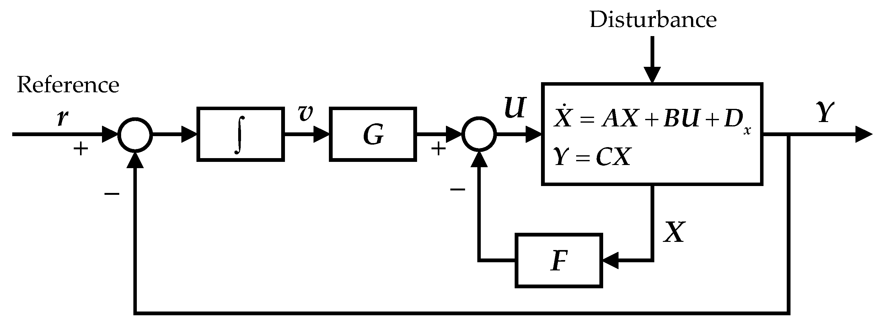
• $X={\left[\begin{array}{cccc}{x}^T& {\phi }^T& {\dot{x}}^T& {\dot{\phi }}^T\end{array}\right]}^T,\hspace{1em}X\in R^n,n=12$ is the state vector;
• $Y={\left[\begin{array}{cc}{x}^T& {\phi }^T\end{array}\right]}^T,\hspace{1em}Y\in R^m,m=6$ is the system output vector;
• $U_a={\left[\begin{array}{cccccccc}{f}_{x1}& f_{x2}& f_{y1}& f_{y2}& f_{z1}& f_{z2}& f_{z3}& f_{z4}\end{array}\right]}^T,U_a\in R^8$ is the control signal vector;
• $D_x$ is the disturbance vector from the bottom plate.

The model parameters and the disturbance vectors are given by Equation (5):

$$\begin{gathered} A=\left[\begin{array}{cc}{O}_6& I_6\\ M^{-1}{A}_1& M^{-1}{A}_2\end{array}\right],\hspace{1em}{B}_A={\left[\begin{array}{cc}{O}_{6\times 8}{}^T& B_a{}^T\end{array}\right]}^T,\hspace{1em}C=\left[\begin{array}{cc}{I}_6& O_6\end{array}\right],\hspace{1em}{D}_x=\left[\begin{array}{cc}{O}_6& O_6\\ M^{-1}{D}_1& M^{-1}{D}_2\end{array}\right]X_b, \\ M=diag\left\{m,m,m,J_{xx},J_{yy},J_{zz}\right\}, \\ {A}_1=\left[\begin{array}{cccccc}-4k_x& 0& 0& 0& 0& 0\\ 0& -4k_y& 0& 0& 0& 0\\ 0& 0& -4k_z& 0& 0& 0\\ 0& -4c{k}_y& 0& -4b^2{k}_z& 0& 0\\ 4c{k}_x& 0& 0& 0& -4a^2{k}_z& 0\\ 0& 0& 0& 0& 0& -4\left(b^2{k}_x+a^2{k}_y\right)\end{array}\right], A_2=\left[\begin{array}{cccccc}-4c_x& 0& 0& 0& 0& 0\\ 0& -4c_y& 0& 0& 0& 0\\ 0& 0& -4c_z& 0& 0& 0\\ 0& -4c{c}_y& 0& -4b^2{c}_z& 0& 0\\ 4c{c}_x& 0& 0& 0& -4a^2{c}_z& 0\\ 0& 0& 0& 0& 0& -4\left(b^2{c}_x+a^2{c}_y\right)\end{array}\right], \\ {B}_a=\left[\begin{array}{cccccccc}1& 1& 0& 0& 0& 0& 0& 0\\ 0& 0& 1& 1& 0& 0& 0& 0\\ 0& 0& 0& 0& 1& 1& 1& 1\\ 0& 0& c+l_{yz}& c+l_{yz}& -l_{zy}& l_{zy}& l_{zy}& -l_{zy}\\ -c-l_{xz}& -c-l_{xz}& 0& 0& -l_{zx}& -l_{zx}& l_{zx}& l_{zx}\\ l_{xy}& -l_{xy}& l_{xz}& -l_{xz}& 0& 0& 0& 0\end{array}\right], \\ {\mathit{X}}_b={\left[\begin{array}{cccc}{x}_b{}^T& {\phi }_b{}^T& {\dot{x}}_b{}^T& {\dot{\phi }}_b{}^T\end{array}\right]}^T, \\ {D}_1=\left[\begin{array}{cccccc}4k_x& 0& 0& 0& 0& 0\\ 0& 4k_y& 0& 0& 0& 0\\ 0& 0& 4k_z& 0& 0& 0\\ 0& 4c{k}_y& 0& 4b^2{k}_z& 0& 0\\ -4c{k}_x& 0& 0& 0& 4a^2{k}_z& 0\\ 0& 0& 0& 0& 0& 4\left(b^2{k}_x+a^2{k}_y\right)\end{array}\right], D_2=\left[\begin{array}{cccccc}4c_x& 0& 0& 0& 0& 0\\ 0& 4c_y& 0& 0& 0& 0\\ 0& 0& 4c_z& 0& 0& 0\\ 0& 4c{c}_y& 0& 4b^2{c}_z& 0& 0\\ -4c{c}_x& 0& 0& 0& 4a^2{c}_z& 0\\ 0& 0& 0& 0& 0& 4\left(b^2{c}_x+a^2{c}_y\right)\end{array}\right] \end{gathered}$$

(5)

where $I_6$ is a 6-by-6 identity matrix and O is a matrix of zeros. The mathematical model shows the presence of mutual interference within the system caused by the allocation of the actuators and the interaction between states. For example, in the first column of ${\mathit{B}}_a$, the motion of the first actuator generates a translation along the x-axis, and at the same time, rotations about the y- and z-axes. The translation along the y-direction is coupled with the rotation about the x-axis, as seen in the second columns of ${\mathit{A}}_1$ and ${\mathit{A}}_2$.

Additionally, the system output obtained from sensors’ measurements is as follows:

$$\begin{gathered} \mathit{Y}\mathbf{=}{\mathit{R}}^{+}{\mathit{Y}}_m\mathbf{,} {\mathit{R}}^{+}={\mathbf{\left(}{\mathit{R}}^T\mathit{R}\mathbf{\right)}}^{-1}{\mathit{R}}^T, \\ {\mathit{Y}}_m={\left[\begin{array}{cccccccc}{x}_1& x_2& y_1& y_2& z_1& z_2& z_4& z_4\end{array}\right]}^T, \\ R=\left[\begin{array}{cccccc}1& 0& 0& 0& -L_{xz}& L_{xy}\\ 1& 0& 0& 0& -L_{xz}& -L_{xy}\\ 0& 1& 0& L_{xz}& 0& L_{zx}\\ 0& 1& 0& L_{xz}& 0& -L_{zx}\\ 0& 0& 1& -L_{zy}& -L_{zx}& 0\\ 0& 0& 1& L_{zy}& -L_{zx}& 0\\ 0& 0& 1& L_{zy}& L_{zx}& 0\\ 0& 0& 1& -L_{zy}& L_{zx}& 0\end{array}\right]\hspace{1em} \end{gathered}$$

(6)

The elements of ${\mathit{Y}}_m$ are the measurements of two horizontal sensors along the x-axis, two horizontal sensors along the y-axis, and four vertical sensors along the z-axis, respectively. The subscript of each measurement corresponds to the nearest actuator.

Proofs for Equations (4)–(6) are given in Appendix A.

Moreover, let an alternative input vector consisting of six elements be as follows:

$$U={\left[\begin{array}{cccccc}{f}_x& f_y& f_z& {\tau }_x& {\tau }_y& {\tau }_z\end{array}\right]}^T\in R^6$$

(7)

where each element of U is the total force/torque in the corresponding direction. Consequently, the control inputs to the eight actuators are computed according to their location and are given by:

$$\begin{array}{l}{U}_a=B_a{}^{+}U,\\ B_a{}^{+}=B_a{}^T{\left(B_a{B}_a{}^T\right)}^{-1}\end{array}$$

(8)

The system dynamics with the new input are given by:

$$\begin{array}{l}\dot{X}=AX+BU+D_x\\ Y=CX\end{array}$$

(9)

with $B={\left[\begin{array}{cc}{O}_6& I_6\end{array}\right]}^T$. The noninteracting control system is then designed so that the interactions between the system states are isolated and the reference in each direction controls the corresponding output.

3. Noninteracting Control Design

3.1. Conditions for a Decoupled Performance

The decoupling process consists of compensating a given system so that each system input independently controls a corresponding system output [9]. The system inputs refer to the references fed to the system. The proposed controller is designed based on a typical integral-type servosystem given by the block diagram illustrated in Figure 2 [20]. The feedback control law is in the following form:

$$U=-FX+Gv\hspace{0.17em}\hspace{0.17em}\hspace{0.17em}\hspace{0.17em}\hspace{0.17em}\hspace{0.17em}\hspace{0.17em}\left(F\in R^{m\times n},G\in R^m\right)$$

(10)

with v a pseudo-state vector defined by the integration of the control error. F and G are controller gains to be designed.

The system dynamics with the feedback control input is represented by:

$$\begin{array}{l}\dot{X}=\left(A-BF\right)X+BGv+D_x\\ Y=CX\end{array}$$

(11)

Let $C_i$ denote the i^th row of the matrix C, and let

$$x_i=\{\begin{array}{l}\min \left\{j|C_i{A}^{j-1}B\ne 0\right\}\hspace{1em}\left(j=1,2,\dots ,n\right)\\ n\hspace{1em}\mathrm{if}\hspace{1em}{C}_i{A}^{j-1}B=0\hspace{0.17em}\mathrm{for}\hspace{0.17em}\mathrm{all}\hspace{0.17em}j\end{array}$$

(12)

The above denotations are characterized by the following:

$$\begin{array}{l}{C}_i{\left(A-BF\right)}^k=C_i{A}^k\hspace{1em}\hspace{1em}\hspace{1em}\hspace{1em}\hspace{1em}\hspace{1em}\hspace{1em}k=0,1,\dots ,x_i-1\\ C_i{\left(A-BF\right)}^k=C_i{A}^{x_i-1}{\left(A-BF\right)}^{k-x_i+1}\hspace{1em}k=x_i,x_i+1,\dots ,n\end{array}$$

(13)

Consider the $i^{th}$ row of the output vector, denoted by $Y_i$, then the following relations between its time-derivatives and the states are obtained as follows:

$$\begin{array}{l}{Y}_i=C_{i}X\\ {\dot{Y}}_i=C_i\dot{X}=C_{i}AX+C_{i}BGv\\ {\ddot{Y}}_i=C_{i}A\dot{X}+C_i\mathit{B}\mathit{G}\dot{v}\\ \hspace{1em}\hspace{0.17em}=C_i{A}^{2}X+C_{i}BG\dot{v}\\ ⋮\\ Y_i^{\left(x_i\right)}=C_i{A}^{x_i-1}\dot{X}+C_{i}BG{v}^{(x_i-1)}\\ \hspace{1em}\hspace{1em}\hspace{0.17em}\hspace{0.17em}=\left(C_i{A}^{x_i}-C_i{A}^{x_i-1}BF\right)X+C_i{A}^{x_i-1}BGv+C_{i}BG{v}^{(x_i-1)}\end{array}$$

(14)

Furthermore, let the following expressions be used:

$$\begin{array}{l}{Y}^{*}={\left[\begin{array}{cccc}{Y}_1^{\left(x_1\right)}& Y_2^{\left(x_2\right)}& \cdots & Y_m^{\left(x_m\right)}\end{array}\right]}^T,\\ A^{*}=\left[\begin{array}{c}{C}_1{A}^{x_1}\\ C_2{A}^{x_2}\\ ⋮\\ C_m{A}^{x_m}\end{array}\right],\hspace{1em}\mathbf{\Delta }=\left[\begin{array}{c}{C}_1{A}^{x_1-1}B\\ C_2{A}^{x_2-1}B\\ ⋮\\ C_m{A}^{x_m-1}B\end{array}\right],\hspace{1em}g=\left[\begin{array}{c}{C}_{1}BG{v}^{(x_1-1)}\\ C_{2}BG{v}^{(x_2-1)}\\ ⋮\\ C_{m}BG{v}^{(x_m-1)}\end{array}\right]\end{array}$$

(15)

Then, from Equations (14) and (15), one can obtain the following:

$$Y^{*}=\left(A^{*}-\mathbf{\Delta }F\right)X+\mathbf{\Delta }Gv+g$$

(16)

If the higher-order term g is neglected, with $\mathbf{\Delta }G$ resulting in a diagonal matrix and $\left(A^{*}-\mathbf{\Delta }F\right)=O$, then the decoupling can be achieved. That is, $x_i$-order time-derivation of ${\mathit{Y}}_i$ depends only on the i^th output error $v_i$ at every system state. Hence, a necessary condition is that the matrix $\mathbf{\Delta }$ should be invertible. Then, a pair of matrices (F, G), which decouples the system, is given by [9,10,16,17]:

$$F={\mathbf{\Delta }}^{-1}{A}^{*},\hspace{0.17em}G={\mathbf{\Delta }}^{-1}$$

(17)

The feedback gain in Equation (17) satisfies the condition of the noninteracting control. However, the stability of the closed-loop system is not guaranteed, and the system performance cannot be satisfied.

3.2. Design of the State Feedback Matrix F

The modified feedback gains such that the system is both decoupled and stable is considered as follows [12]:

$$F={\mathbf{\Delta }}^{-1}\left(A^{*}+\overline{F}{S}_a\right)$$

(18)

where $\overline{F}$ is a feedback matrix to be tuned such that the closed-loop system is asymptotically stable, and ${\mathit{S}}_a$ is given by the following nonsingular matrix:

$$S_a=\left[\begin{array}{c}{C}_1\\ ⋮\\ C_1{A}^{x_1-1}\\ C_2\\ ⋮\\ C_2{A}^{x_2-1}\\ ⋮\\ \begin{array}{c}{C}_m{A}^{x_m-1}\\ W\end{array}\end{array}\right]\in R^{n\times n},\hspace{1em}\mathrm{with}\hspace{1em}\left[\begin{array}{c}{C}_1\\ ⋮\\ C_1{A}^{x_1-1}\\ C_2\\ ⋮\\ C_2{A}^{x_2-1}\\ ⋮\\ C_m{A}^{x_m-1}\end{array}\right]\in R^{\left(m+{\displaystyle \sum _{i=1}^m\left(x_i-1\right)}\right)\times n}\hspace{1em}\mathrm{and}\hspace{1em}WB=O$$

(19)

Substituting Equation (18) into Equation (16) and neglecting the higher-order term yields the following:

$$Y^{*}=-\left(\overline{F}{S}_a\right)X+v$$

(20)

Therefore, the $i^{th}$ row of ${\mathit{Y}}^{*}$ is given by the following:

$$Y_i^{\left(x_i\right)}=-\left({\overline{F}}_i{S}_a\right)X+v_i$$

(21)

where ${\overline{F}}_i$ is the corresponding i^th row of $\overline{F}$. ${\overline{F}}_i$ can be represented as in Equation (22):

$${\overline{F}}_i=\left[\begin{array}{cccc}\underset{{\overline{F}}_{i1}}{\underbrace{\begin{array}{ccc}{f}_{10}& \cdots & f_{1\left(x_1-1\right)}\end{array}}}& \underset{{\overline{F}}_{i2}}{\underbrace{\begin{array}{ccc}{f}_{20}& \cdots & f_{2\left(x_2-1\right)}\end{array}}}& \cdots & \underset{{\overline{F}}_{im}}{\underbrace{\begin{array}{cc}\cdots & f_{m\left(x_m-1\right)}\end{array}}}\end{array}{f}_w\right]$$

(22)

Then, substituting Equations (19) and (22) into Equation (21) yields:

$$\begin{array}{l}-Y_i^{\left(x_i\right)}={\overline{F}}_{i1}{C}_1\left[\begin{array}{c}I\\ ⋮\\ A^{x_1-1}\end{array}\right]X+{\overline{F}}_{i2}{C}_2\left[\begin{array}{c}I\\ ⋮\\ A^{x_2-1}\end{array}\right]X+\cdots +{\overline{F}}_{im}{C}_m\left[\begin{array}{c}I\\ ⋮\\ A^{x_m-1}\end{array}\right]X+f_{w}WX+v_i\\ \hspace{1em}\hspace{1em}={\overline{F}}_{i1}\left(\left[\begin{array}{c}{Y}_1\\ ⋮\\ Y_1{}^{\left(x_1-1\right)}\end{array}\right]+\left[\begin{array}{c}0\\ ⋮\\ C_{1}BG{v}^{\left(x_1-2\right)}\end{array}\right]\right)+{\overline{F}}_{i2}\left(\left[\begin{array}{c}{Y}_2\\ ⋮\\ Y_2{}^{\left(x_2-1\right)}\end{array}\right]+\left[\begin{array}{c}0\\ ⋮\\ C_{2}BG{v}^{\left(x_2-2\right)}\end{array}\right]\right)+\cdots +f_{w}WX+v_i\end{array}$$

(23)

If the matrix $\overline{F}$ satisfies the following conditions, it can be considered a solution for the decoupling problem:

$$\{\begin{array}{l}{\overline{F}}_{ij}=0\hspace{1em}\mathrm{if}\hspace{1em}j\ne i\\ {\overline{F}}_{ij}\ne 0\hspace{1em}\mathrm{if}\hspace{1em}j=i\end{array}$$

(24)

The value of ${\overline{F}}_{ii}$ can be designed using classical approaches, such as the pole placement technique. Note that the number of the closed-loop poles (p) can be specified while decoupling the control system, and the number of free parameters (f) in a decoupling matrix $\overline{\mathit{F}}$ is given by [21]:

$$\begin{array}{l}m+{\displaystyle \sum _1^m\left(x_i-1\right)}\le p\le n\\ m+{\displaystyle \sum _1^m\left(x_i-1\right)}\le f\end{array}$$

(25)

3.3. The LMI-Based Design of the Feedback Matrix G

Since several elements of the state feedback matrix are neglected in order to identify the decoupled control law, the system performance may be affected. The matrix G from Equation (17) should be modified to achieve the desired performances and its modified expression is given by:

$$G={\mathbf{\Delta }}^{-1}\overline{\mathit{G}}$$

(26)

with $\overline{\mathit{G}}$, a diagonal matrix, chosen so that the decoupling characteristics are preserved. Substituting F (Equation (18)) and G (Equation (26)) into the system model (Equation (11)), the closed-loop system is obtained as follows:

$$\begin{array}{l}\dot{\tilde{X}}=\left[\begin{array}{c}\dot{X}\\ \dot{v}\end{array}\right]=\underset{\tilde{A}}{\underbrace{\left[\begin{array}{cc}A-B\left({\mathbf{\Delta }}^{-1}{A}^{*}+\overline{F}{S}_a\right)& O_6\\ -C& O_6\end{array}\right]}}\tilde{X}+\underset{\tilde{B}}{\underbrace{\left[\begin{array}{c}B{\mathbf{\Delta }}^{-1}\\ O_6\end{array}\right]}}\underset{\tilde{K}}{\underbrace{\left[\begin{array}{cc}{O}_{12\times 6}& \overline{G}\end{array}\right]}}\tilde{X}+\underset{d}{\underbrace{\left[\begin{array}{c}{D}_x\\ r\end{array}\right]}}\\ \tilde{Y}=\underset{\tilde{C}}{\underbrace{\left[\begin{array}{cc}{O}_{6\times 12}& I_6\end{array}\right]}}\tilde{X}\end{array}$$

(27)

If there exists a $Z\in {\mathit{R}}^{6\times 18}$ and a $Q\in R^{18\times 18}(>0)$ that follow, respectively, the following forms:

$$\begin{array}{l}\mathit{Z}=\left[\begin{array}{cc}{\mathit{O}}_{6\times 12}& {\mathit{Z}}_3\end{array}\right]\\ \mathit{Q}=\left[\begin{array}{lll}{\mathit{Q}}_{11}& {\mathit{Q}}_{12}& {\mathit{Q}}_{13}\\ {\mathit{Q}}_{21}& {\mathit{Q}}_{22}& {\mathit{Q}}_{23}\\ {\mathit{O}}_6& {\mathit{O}}_6& {\mathit{Q}}_{33}\end{array}\right],{\mathit{Q}}_{ij}\in {\mathit{R}}^{6\times 6},\\ {\mathit{Z}}_3\hspace{0.17em}\mathrm{and}\hspace{0.17em}{\mathit{Q}}_{33}\hspace{0.17em}\mathrm{are}\hspace{0.17em}\mathrm{diagonal}\hspace{0.17em}\mathrm{matrices}.\end{array}$$

(28)

If there exist γ > 0 such that the following LMI is feasible:

$$\left[\begin{array}{cc}\tilde{A}Q+Q{\tilde{A}}^T+\tilde{B}Z+Z^T{\tilde{B}}^T+I& Q{\tilde{C}}^T\\ \tilde{C}Q& -{\gamma }^{2}I\end{array}\right]\le 0$$

(29)

Then, the state feedback gain, given by:

$$\tilde{\mathit{K}}=Z{Q}^{-1}$$

(30)

ensures that the ${\mathit{L}}_2$ gain of the system described by $\underset{{\Vert d\Vert }_2\ne 0}{\sup }({\Vert \tilde{Y}\Vert }_2/{\Vert d\Vert }_2)$ is less than $\gamma$ [22]. Minimizing $\gamma$ over the variables Z and Q results in the smallest upper bound on the ${\mathit{L}}_2$ gain of the system.

Moreover, from Equations (27) and (30), the following is deduced:

$$\begin{array}{l}Z=\tilde{\mathit{K}}Q=\left[\begin{array}{cc}{O}_{6\times 12}& \overline{G}{Q}_{33}\end{array}\right]\\ \Rightarrow \overline{G}=Z_3{Q}_{33}^{-1}\end{array}$$

(31)

and since both ${\mathit{Z}}_3$ and ${\mathit{Q}}_{33}$ are diagonal matrices, $\overline{\mathit{G}}$ is also diagonal. Thus, the decoupled characteristics are guaranteed.

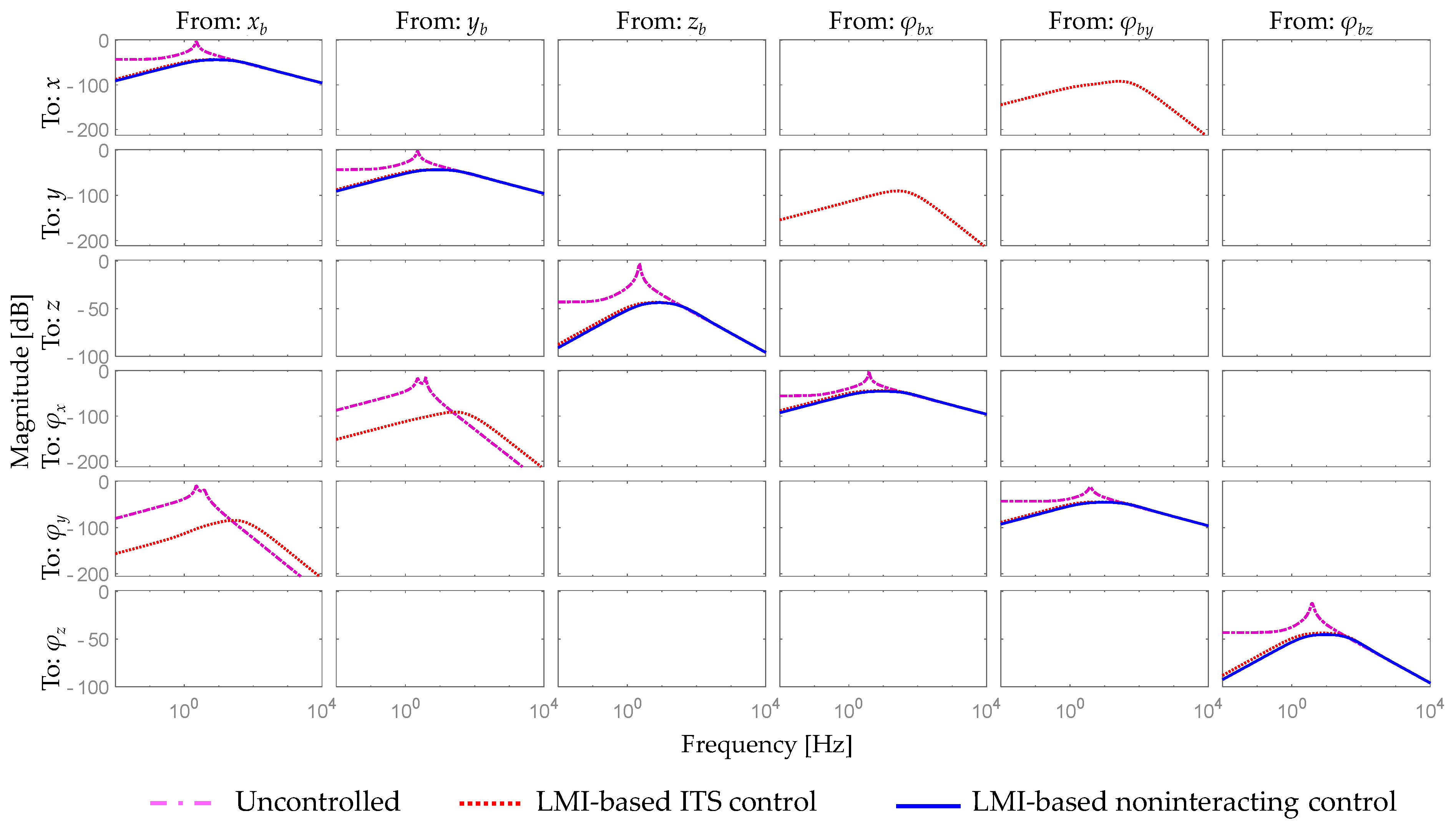
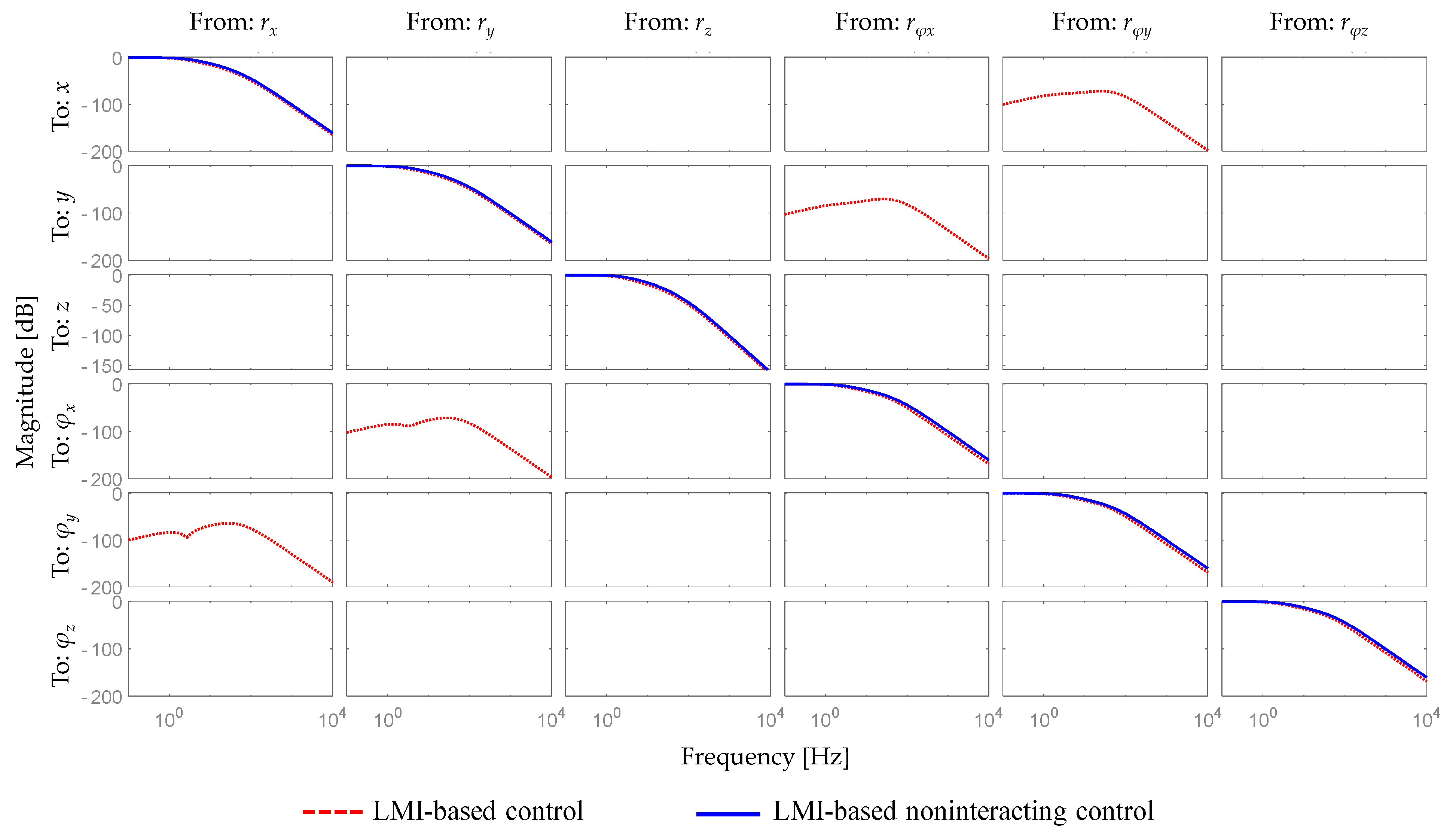
4. Simulation Studies

4.1. Implementation

The specifications of the AVIS are listed in

Table 1. Specifications of the controlled AVIS.

Parameter	Value	Parameter	Value	Parameter	Value
a [m]	0.4	m [kg]	288	lzy [m]	0.53
b [m]	0.6	Jxx [kg.m2]	34.8	lxz [m]	0.015
c [m]	0.2	Jyy [kg.m2]	15.6	lzx [m]	0.37
kx, ky, kz [N/m]	14,180	Jzz [kg.m2]	49.92	lxy [m]	0.53
cx, cy, cz [Ns/m]	100	lxx [m]	0.29	lyz [m]	0.015

, and the matrix gains of the system model were obtained accordingly. With these values, the matrix $\mathbf{\Delta }$ was computed and confirmed to be nonsingular. Thus, the noninteracting controller was designed. The state feedback matrix F, given in Equation (18), was identified. Using the Robust Control Toolbox in Matlab, the LMI given by Equation (29) with the predefined conditions from Equation (28) was solved for the AVIS with a minimal value of $\gamma$ of 0.08. $\overline{\mathit{G}}$ was identified afterward from Equation (31), and subsequently, G was obtained from Equation (26). The two control matrices are presented in Equation (32).

$$\begin{gathered} \begin{array}{l}F=[\begin{array}{cccccc}44984006.525& 0& 0& 0& 0& 0\\ 0& 44988623.006& 0& 0& 0& 0\\ 0& 0& 44981212.885& 0& 0& 0\\ 0& -2836& 0& 5680686.115& 0& 0\\ 2836& 0& 0& 0& 2547779.731& 0\\ 0& 0& 0& 0& 0& 8151470.398\end{array}\cdots \\ \hspace{0.17em}\hspace{0.17em}\hspace{0.17em}\hspace{0.17em}\hspace{0.17em}\hspace{0.17em}\hspace{0.17em}\hspace{0.17em}\hspace{0.17em}\hspace{0.17em}\hspace{0.17em}\hspace{0.17em}\hspace{0.17em}\hspace{0.17em}\hspace{0.17em}\hspace{0.17em}\hspace{0.17em}\hspace{0.17em}\hspace{0.17em}\hspace{0.17em}\hspace{0.17em}\hspace{0.17em}\hspace{0.17em}\hspace{0.17em}\hspace{0.17em}\hspace{0.17em}\hspace{0.17em}\hspace{0.17em}\hspace{0.17em}\hspace{0.17em}\begin{array}{cccccc}285212.077& 0& 0& 0& 0& 0\\ 0& 285243.371& 0& 0& 0& 0\\ 0& 0& 285186.983& 0& 0& 0\\ 0& 0& 0& 30735.931& 0& 0\\ 4& 0& 0& 0& 13697.327& 0\\ 0& 0& 0& 0& 0& 44134.904\end{array}]\\ \hspace{0.17em}\hspace{0.17em}\hspace{0.17em}\hspace{0.17em}\hspace{0.17em}\hspace{0.17em}\hspace{0.17em}\hspace{0.17em}\hspace{0.17em}\hspace{0.17em}\hspace{0.17em}\hspace{0.17em}\hspace{0.17em}\hspace{0.17em}\hspace{0.17em}\hspace{0.17em}\hspace{0.17em}\hspace{0.17em}\hspace{0.17em}\hspace{0.17em}\hspace{0.17em}\hspace{0.17em}\hspace{0.17em}\hspace{0.17em}\hspace{0.17em}\hspace{0.17em}\hspace{0.17em}\hspace{0.17em}\hspace{0.17em}\hspace{0.17em}\hspace{0.17em}\hspace{0.17em}\hspace{0.17em}\end{array} \\ G=\left[\begin{array}{cccccc}644291218.410& 0& 0& 0& 0& 0\\ 0& 644343230.526& 0& 0& 0& 0\\ 0& 0& 644258432.699& 0& 0& 0\\ 0& 0& 0& 81818216.496& 0& 0\\ 0& 0& 0& 0& 36687353.269& 0\\ 0& 0& 0& 0& 0& 117422614.479\end{array}\right] \end{gathered}$$

(32)

Moreover, another state feedback controller was designed to provide a fair assessment of the control system proposed in this paper. This controller was also designed based on the integral-type servo system, illustrated in Figure 2. The state-space representation of the closed-loop system is given in Equation (33).

$$\begin{array}{l}\dot{\tilde{X}}=\left[\begin{array}{c}\dot{X}\\ \dot{v}\end{array}\right]=\underset{\underset{\_}{A}}{\underbrace{\left[\begin{array}{cc}A& O_6\\ -C& O_6\end{array}\right]}}\tilde{X}+\underset{\underset{\_}{B}}{\underbrace{\left[\begin{array}{c}B\\ O_6\end{array}\right]}}U+\underset{d}{\underbrace{\left[\begin{array}{c}{D}_x\\ r\end{array}\right]}}\\ \tilde{Y}=\tilde{C}\tilde{X}\\ U=-\underset{\_}{F}X+\underset{\_}{G}v\end{array}$$

(33)

Accordingly, the following LMIs were considered:

$$\begin{array}{l}\left[\begin{array}{cc}\underset{\_}{A}\underset{\_}{Q}+\underset{\_}{Q}{\underset{\_}{A}}^T+\underset{\_}{B}\underset{\_}{Z}+{\overline{Z}}^T{\underset{\_}{B}}^T+I& \underset{\_}{Q}{\underset{\_}{C}}^T\\ \underset{\_}{C}\underset{\_}{Q}& -{\gamma }^{2}I\end{array}\right]\le 0\\ \underset{\_}{Z}>0,\hspace{0.17em}\underset{\_}{Z}\in R^{6\times 18}\\ \underset{\_}{Q}>0,\hspace{0.17em}\underset{\_}{Q}\in R^{18}\end{array}$$

(34)

The feedback control gains were obtained such as $\left[\begin{array}{cc}\underset{\_}{F}& \underset{\_}{G}\end{array}\right]=\underset{\_}{Z}{\underset{\_}{Q}}^{-1}$. Their values are presented in Equation (35).

$$\begin{gathered} \begin{array}{l}\underset{\_}{F}=[\begin{array}{cccccc}23055996.125& 0& 0& 0& -451615.356& 0\\ 0& 23037296.982& 0& 343167.966& 0& 0\\ 0& 0& 23020562.484& 0& 0& 0\\ 0& -48722.485& 0& 331246.305& 0& 0\\ 52733.158& 0& 0& 0& 226948.799& 0\\ 0& 0& 0& 0& 0& 500955.474\end{array}\cdots \\ \hspace{0.17em}\hspace{0.17em}\hspace{0.17em}\hspace{0.17em}\hspace{0.17em}\hspace{0.17em}\hspace{0.17em}\hspace{0.17em}\hspace{0.17em}\hspace{0.17em}\hspace{0.17em}\hspace{0.17em}\hspace{0.17em}\hspace{0.17em}\hspace{0.17em}\hspace{0.17em}\hspace{0.17em}\hspace{0.17em}\hspace{0.17em}\hspace{0.17em}\hspace{0.17em}\hspace{0.17em}\hspace{0.17em}\hspace{0.17em}\hspace{0.17em}\hspace{0.17em}\hspace{0.17em}\hspace{0.17em}\hspace{0.17em}\hspace{0.17em}\hspace{0.17em}\hspace{0.17em}\hspace{0.17em}\begin{array}{cccccc}66660.618& 0& 0& 0& -1121.874& 0\\ 0& 66606.378& 0& 863.757& 0& 0\\ 0& 0& 66560.178& 0& 0& 0\\ 0& -145.165& 0& 803.471& 0& 0\\ 156.715& 0& 0& 0& 526.273& 0\\ 0& 0& 0& 0& 0& 1231.046\end{array}]\end{array} \\ \underset{\_}{G}=\left[\begin{array}{cccccc}242833691.013& 0& 0& 0& -4787897.103& 0\\ 0& 242637163.198& 0& 3633362.131& 0& 0\\ 0& 0& 242461475.407& 0& 0& 0\\ 0& -508721.625& 0& 3530889.292& 0& 0\\ 550890.757& 0& 0& 0& 2420898.234& 0\\ 0& 0& 0& 0& 0& 5336827.751\end{array}\right] \end{gathered}$$

(35)

4.2. Simulations

The performance of the proposed noninteracting controller was evaluated through two simulation tasks: vibration isolation and platform positioning. The results of these simulations were compared to those of the integral-type servo (ITS) control system. For the former task, the top plate of the AVIS has to be isolated from any vibration source. In practical applications, most of these vibrations are transmitted through the floor and are mainly the result of machines operating in the same workspace. Thus, the control system needs to suppress the ground vibrations in any direction and, while doing so, the actuators should not generate any unwanted motions in the other directions. Meanwhile, in the latter task, the top plate of the AVIS is expected to approach a set-point in any direction without affecting the motion of other directions. In other words, the matrix representing the relationship between the reference and the output should be diagonal.

Figure 3 shows the vibration isolation frequency response against the vibration from the bottom plate that is fixed to the ground. Each column of graphs represents the motion of the top plate in respect to the vibration of the bottom plate in that specific direction. As illustrated in this figure, the mass-spring-damper systems, in their nature, are capable of suppressing vibrations, especially high-frequency vibrations. Unfortunately, the resonance phenomenon is unavoidable with the passive systems—the peak in each frequency response. Moreover, a vibration along the $x_b$-axis of the ground results in a translation in the same direction and an additional rotation about the y-axis of the top plate, as shown in the first column of Figure 3. Similarly, vibrations along the $y_b$-axis generate a translation along the y-axis and a rotation along the φ_x direction.

Using both control strategies, the performance of the system at low-frequency ranges had improved significantly. Unfortunately, the integral-type servo controller, similar to the uncontrolled case, generated unwanted rotations while suppressing the translations from the bottom plate along the x- and y-axes. Furthermore, undesired translations appeared during the suppression of rotational vibrations, as shown in the fourth and fifth columns of Figure 3. On the other hand, the proposed noninteracting controller provided good isolation performance without creating any unwanted motions. Therefore, in Figure 3, the response of the noninteracting control system appears only at the graphs on the main diagonal line.

In Figure 4, the time response showcases further the efficiency of the proposed control system. The bottom plate is supposed to perform step-type movements of 0.01 (m) or 0.01 (rad) in different directions at different times. The mutual interference between the DoFs of the AVIS can be clearly seen in the bottom-left sub-figure of Figure 4a, with rotations appearing along with the translational movements. Aside from using the ITS control system, unwanted motions can be seen in the zoomed sub-figures in Figure 4b. On the other hand, unwanted motions of any direction affected by other directions’ motions were not or hardly generated when the noninteracting control was used. The differentiations of these results were caused by the resulting system configuration decoupling the mutual interference within the system with the noninteracting control law. In other words, the proposed controller isolated the vibrations and decoupled the interactions of the system effectively and swiftly without generating any undesired motions.

Figure 5 shows the frequency response of the system for the positioning task. Each column illustrates the Bode magnitude plots of the system response in every direction in response to the corresponding reference. Accordingly, the i^th entry of the graphs on the main diagonal line depicts the complementary sensitivity from the reference $r_i$ and the output ${\mathit{Y}}_i$. All entries outside the diagonal line are unwanted motions resulting from the interactions within the system. As illustrated in this figure, the proposed controller decouples these interactions effectively while providing good positioning performances. On the other hand, the ITS control system controller generates undesirable motions, and the vibration isolation has thus deteriorated.

5. Conclusions

In this paper, the authors suggested an effective control strategy for 6-DoF AVIS. This study focused on the configuration of the control system for this complex dynamic plant based on the concept of the noninteracting control design. The resulting closed-loop system was represented with a completely diagonal structure; that is, each output is independently controlled by the corresponding reference signal. The analytical methodology of deriving the noninteracting controller was proposed, and the optimal control law was obtained using the LMI technique. In addition, an ITS control system was designed to compare its performance with the proposed controller.

The efficiency of the proposed control system was evaluated through two sets of simulations: vibration isolation and platform positioning. According to these simulation tests, the vibration isolation performance of both control schemes at low-frequency ranges improved significantly. However, the ITS control system generated additional and unwanted translations and rotations, whereas the proposed noninteracting controller isolated the AVIS without creating any additional motions. Similar results were obtained in the platform positioning simulation test. The analysis of the Bode magnitude plots revealed the interaction between the DoFs of the AVIS, especially with the ITS control system. On the other hand, the simulation results using the noninteracting controller proved the efficiency of this controller in decoupling the mutual interferences effectively while providing good positioning performances.

In future work, an experimental study will be conducted with the proposed control system to evaluate the vibration isolation performances.

References

- Tuo, J.; Deng, Z.; Huang, W.; Zhang, H. A six degree of freedom passive vibration isolator with quasi-zero-stiffness-based supporting. J. Low Freq. Noise Vib. Act. Control 2018, 37, 279–294. [Google Scholar] [CrossRef] [Green Version]
- Sun, J.O.; Kim, K.J. Six-degree of freedom active pneumatic table based on time delay control technique. Proc. Inst. Mech. Eng. Part I J. Syst. Control Eng. 2012, 226, 622–637. [Google Scholar] [CrossRef]
- Nakamura, Y.; Nakayama, M.; Yasuda, M.; Fujita, T. Development of active six-degrees-of-freedom micro-vibration control system using hybrid actuators comprising air actuators and giant magnetostrictive actuators. Smart Mater. Struct. 2006, 15, 1133–1142. [Google Scholar] [CrossRef]
- Kang, S.; Wu, H.; Yang, X.; Li, Y.; Wang, Y. Fractional-order robust model reference adaptive control of piezo-actuated active vibration isolation systems using output feedback and multi-objective optimization algorithm. J. Vib. Control 2020, 26, 19–35. [Google Scholar] [CrossRef]
- Jiang, D.; Li, J.; Li, X.; Deng, C.; Liu, P. Modeling identification and control of a 6-DOF active vibration isolation system driving by voice coil motors with a Halbach array magnet. J. Mech. Sci. Technol. 2020, 34, 617–630. [Google Scholar] [CrossRef]
- Chen, Y.-D.; Fuh, C.C.; Tung, P.C. Application of voice coil motors in active dynamic vibration absorbers. IEEE Trans. Magn. 2005, 41, 1149–1154. [Google Scholar] [CrossRef]
- Kim, H.J.; Lee, D.H.; Park, H.C.; Kim, Y.B. Direct Disturbance Suppression System Design for High Precision Fabrication Tables. Trans. Korean Soc. Mech. Eng. A 2020, 44, 843–853. [Google Scholar] [CrossRef]
- Kim, M.H.; Kim, H.Y.; Kim, H.C.; Ahn, D.; Gweon, D.G. Design and Control of a 6-DOF active vibration isolation system using a halbach magnet array. IEEE/ASME Trans. Mechatron. 2016, 21, 2185–2196. [Google Scholar] [CrossRef]
- Kucera, V. Diagonal Decoupling of Linear Systems by Static-State Feedback. IEEE Trans. Autom. Control 2017, 62, 6250–6265. [Google Scholar] [CrossRef]
- Morse, A.; Wonham, W. Status of noninteracting control. IEEE Trans. Autom. Control 1971, 16, 568–581. [Google Scholar] [CrossRef]
- Bonilla, M.; Pallottino, L.; Bicchi, A. Noninteracting constrained motion planning and control for robot manipulators. In Proceedings of the 2017 IEEE International Conference on Robotics and Automation (ICRA), Singapore, 29 May–3 June 2017; pp. 4038–4043. [Google Scholar]
- Kim, Y.-B. An algorithm for robust noninteracting control of ship propulsion system. KSME Int. J. 2000, 14, 393–400. [Google Scholar] [CrossRef]
- Liu, H.; Duan, G. Input-output Energy Decoupling Control for Linear Neutral Time-delay Systems. In Proceedings of the 2006 6th World Congress on Intelligent Control and Automation, Dalian, China, 21–23 June 2006; Volume 1, pp. 2353–2357. [Google Scholar]
- Chu, D.; Tan, R.C.E. Numerically Reliable Computing for the Row by Row Decoupling Problem with Stability. SIAM J. Matrix Anal. Appl. 2002, 23, 1143–1170. [Google Scholar] [CrossRef]
- Jayawardhana, B. Noninteracting control of nonlinear systems based on relaxed control. In Proceedings of the 49th IEEE Conference on Decision and Control (CDC), Atlanta, GA, USA, 15–17 December 2010; pp. 7087–7091. [Google Scholar]
- Freund, E. Design of time-variable multivariable systems by decoupling and by the inverse. IEEE Trans. Autom. Control 1971, 16, 183–185. [Google Scholar] [CrossRef]
- Porter, W. Decoupling of and inverses for time-varying linear systems. IEEE Trans. Autom. Control 1969, 14, 378–380. [Google Scholar] [CrossRef]
- Falb, P.; Wolovich, W. Decoupling in the design and synthesis of multivariable control systems. IEEE Trans. Autom. Control 1967, 12, 651–659. [Google Scholar] [CrossRef] [Green Version]
- Niku, S.B. Introduction to Robotics: Analysis, Control, Applications; John Wiley & Sons: New York, NY, USA, 2020. [Google Scholar]
- FUJISAKI, Y.; IKEDA, M. Synthesis of Two-Degree-of-Freedom Optimal Servosystems. Trans. Soc. Instrum. Control Eng. 1991, 27, 907–914. [Google Scholar] [CrossRef]
- Christodoulou, M.A. Decoupling in the design and synthesis of singular systems. Automatica 1986, 22, 245–249. [Google Scholar] [CrossRef]
- Boyd, S.; El Ghaoui, L.; Feron, E.; Balakrishnan, V. Linear Matrix Inequalities in System and Control Theory; Society for Industrial and Applied Mathematics: Philadelphia, PA, USA, 1994; ISBN 978-0-89871-485-2. [Google Scholar]