On Unmanned Aerial Vehicles Light Show Systems: Algorithms, Software and Hardware

Abstract

Unmanned aerial vehicle (UAV) light shows (UAV-LS) have a wow factor due to their advantages in terms of environment friendliness and controllability compared to traditional fireworks. In this paper, a UAV-LS system is developed including a collision-free formation transformation trajectory planning algorithm, a software package that facilitates animation design and real-time monitoring and control, and hardware design and realization. In particular, a dynamic task assignment algorithm based on graph theory is proposed to reduce the impact of UAV collision avoidance on task assignment and the frequency of task assignment in the formation transformation. In addition, the software package consists of an animation interface for formation drawing and 3D animation simulation, which helps the monitoring and control of UAVs through a real-time monitoring application. The developed UAV-LS system hardware consists of subsystems of decision-making, real-time kinematic (RTK) global positioning system (GPS), wireless communication, and UAV platforms. Outdoor experiments using six quadrotors are performed and details of implementations of high-accuracy positioning, communication, and computation are presented. Results show that the developed UAV-LS system can successfully complete a light show and the proposed task assignment algorithm performs better than traditional static ones.

1. Introduction

Unmanned aerial vehicle (UAV) light shows (UAV-LS) are an emerging technology for festivals and company promotions. Compared with traditional fireworks, UAV-LS are environmentally friendly and more flexible to present animations. With the rapid advancement of UAVs and their control technologies, successful UAV-LS cases can be found, manufactured by various companies such as Intel and Ehang [1,2]. As a result, studies of swarm control, communication, planning, and software and hardware design are becoming increasingly popular for more intelligent, energy-efficient, and beautiful light shows.

There are many ways to control a group of UAVs, e.g., using a brain–computer interface (BCI) [3] or a ground control station (GCS). In most UAV-LS systems, a ground control station, e.g., a high-performance computer or mobile device, is responsible for managing and controlling the UAVs [4]. Depending on the degree of intervention from the GCS, UAV-LS systems can be operated under three modes, i.e., man-in-the-loop, semi-autonomous, and autonomous [5,6]. In the man-in-the-loop mode, UAVs are completely controlled by the GCS during the light show. In the semi-autonomous mode, the onboard flight controller, which maintains the flight stability and avoids collisions, cooperates with the GCS. In the autonomous mode, UAVs can autonomously make decisions and plan their paths. In the context of a light show, there is a necessary trade-off between the cost of hundreds or even thousands of UAVs and the control performance. Indeed, the success of the autonomous mode heavily relies on powerful onboard computing units and sensors, which are extremely expensive for a large-scale UAV group. As a result, the semi-autonomous mode is considered in this paper as an affordable and competitive solution. In such mode, the GCS sends way-point information to UAVs and the onboard flight controller tracks the way-point and then sends back the status of the UAVs. Since UAV-LS systems usually perform in fixed and limited airspace, the increasing demand of communications among UAVs and the GCS in the semi-autonomous mode would not result in significant expense growth.

One of the key steps in the process of a UAV-LS is formation transformation, where UAVs move from an initial formation to a target one in order to switch light graphics in the air. To do so, the task assignment problem (TAP) must first be tackled, which in essence states that each node in the target formation should be assigned to a UAV in order to satisfy a pre-defined criteria, e.g., minimum total flight distance. Then, the trajectory planning problem must be considered to generate smooth and collision-free trajectories for safety concerns. Studies on these problems have been reported by many researchers. In [7,8,9], path planning and obstacle avoidance algorithms for a single UAV have been reviewed. In [10,11], the particle swarm optimization (PSO) algorithm has been employed to solve the TAP without collision avoidance. In [12], a discrete wolf pack algorithm is proposed to solve the multi-UAV task assignment with fast convergence speed. In [13], Duan et al. present a multi-UAV formation reconfiguration algorithm based on the hybrid PSO and genetic algorithm (HPSOGA) to achieve formation transformation while satisfying various formation constraints. In [14,15], a distributed cooperative control method is proposed to realize the desired formation without task assignment and collision avoidance. In [16], a UAVs-LS system is realized to achieve precise formation and coordination control using multi-UAV teaming technologies. However, in the aforementioned works, the TAP and the trajectory planning problem are decoupled, such that the TAP generates straight-line trajectories from the initial node to the target one. Yet in practice, UAVs often deviate from the straight-line trajectories due to mutual collision avoidance and external disturbances, leading to a mismatch between the actual task execution cost and the desired one.

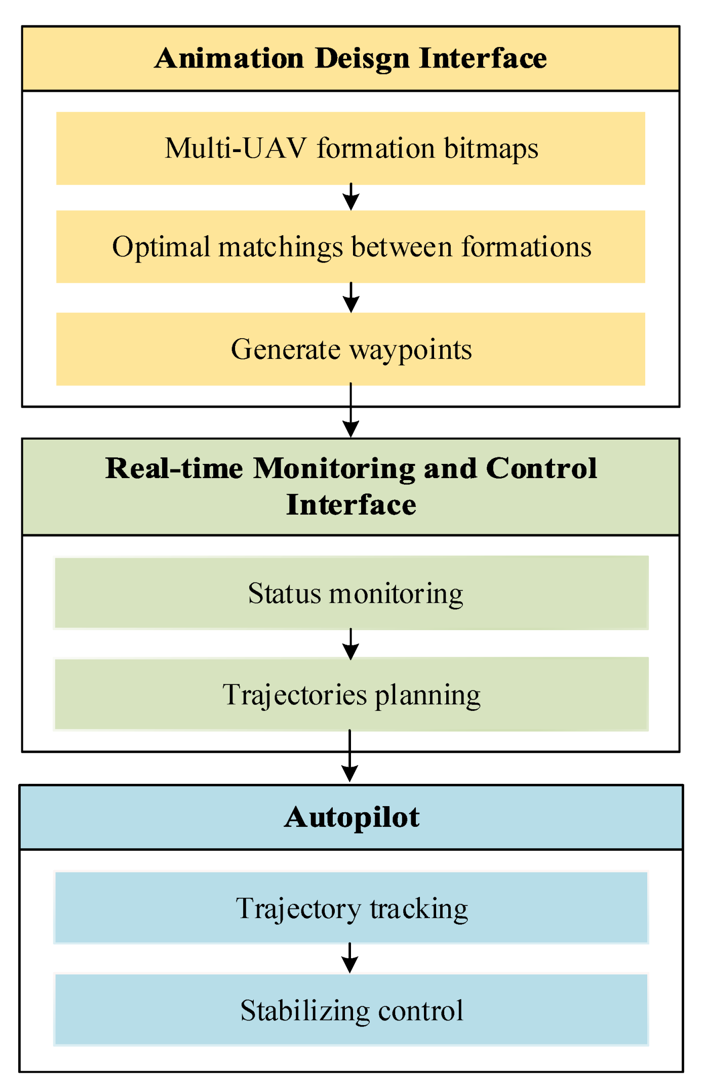
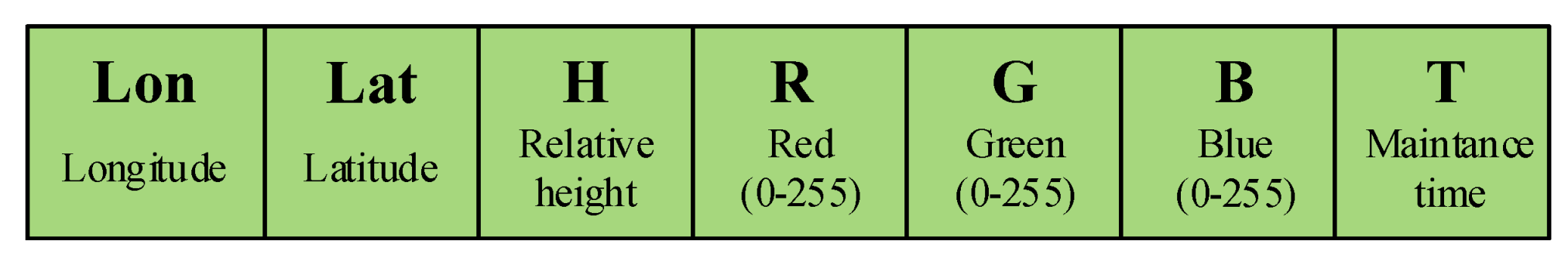
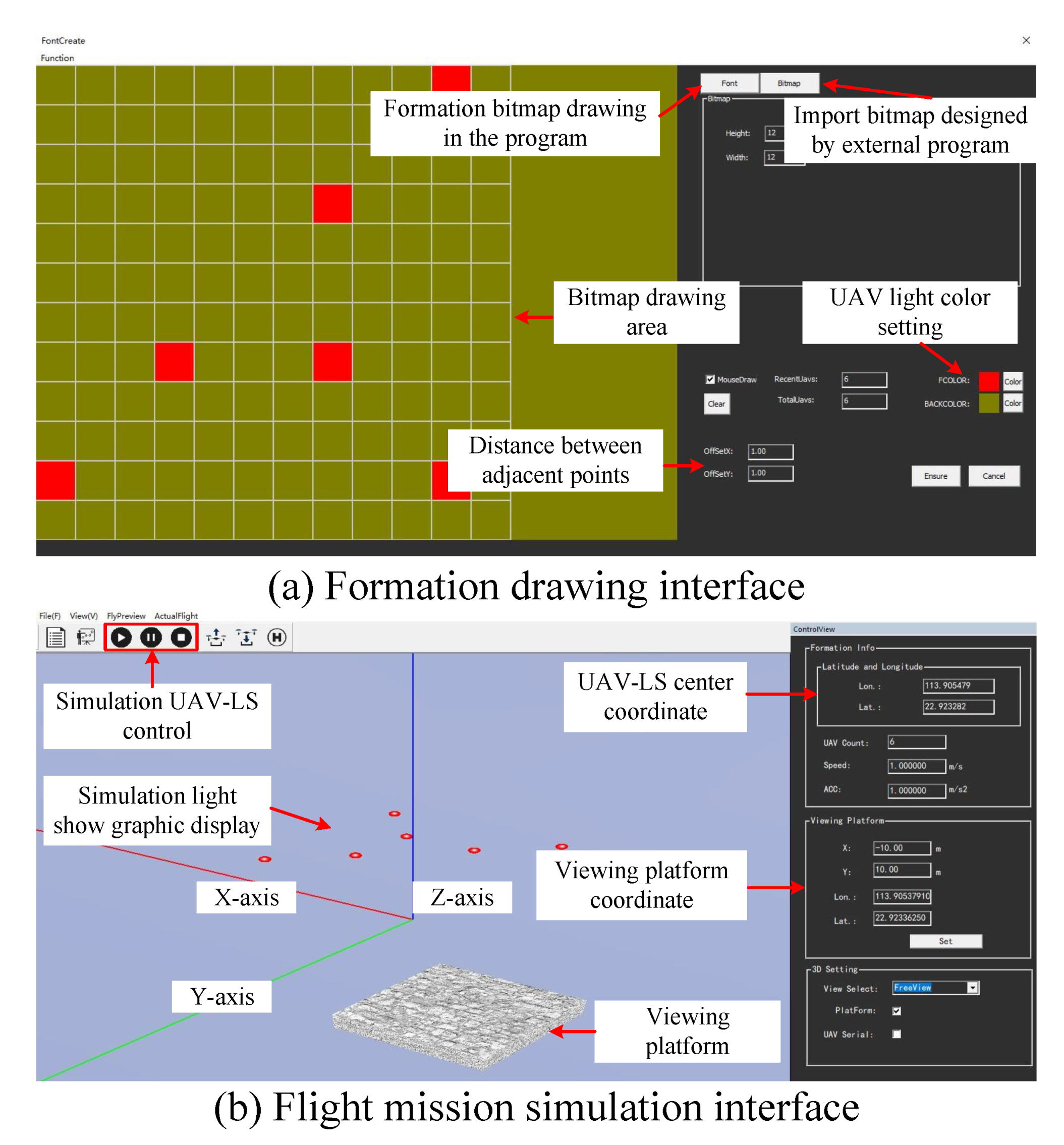
In this paper, we present a UAV-LS system including a dynamic collision-free formation transformation algorithm, a software package that consists of an animation design interface (ADI) and a real-time monitoring application, and a complete hardware design and realization. The proposed formation transformation algorithm dynamically solves the TAP in a conditional-triggering way and constructs repulsion field around obstacles to avoid inter-collisions of UAVs. Compared with the traditional static task assignment methods, the TAP is not only solved offline to obtain an initial task assignment with the minimum total flight distance of all UAVs, but is also dynamically solved online to consider the impact of real-time trajectory deviation due to collision avoidance. The collision avoidance between UAVs is set as a trigger condition to reduce the frequency of dynamic task assignment, and the TAP is only solved within a group of local UAVs to avoid a high computational cost of solving a global TAP. In addition, formation drawing and 3D animation simulations are provided in the ADI to facilitate the animation design process. During the light show, the monitoring and control of UAVs is conducted through the real-time monitoring application. The UAV-LS hardware consists of subsystems of decision-making, real-time kinematic (RTK) global positioning system (GPS), wireless communication, and UAV platforms. The UAV platform is made up of a number of homogeneous quadrotors without onboard collision avoidance sensors for economic reasons. Finally, outdoor experiments using six quadrotors are performed. Details of implementations of centimeter-level positioning, communication and computation are given. Results show that the developed UAV-LS system can successfully complete a light show, and the proposed algorithm is better than the traditional static task assignment one in terms of scalability, efficiency, and performance.

The remainder of this paper is organized as follows. In Section 2, the formation transformation algorithm is introduced. Section 3 introduces the software package developed for the UAVs-LS. Section 4 provides details of the self-developed quadrotor prototype and the UAVs-LS system. The simulations of proposed formation transformation algorithm and experiments of UAV-LS are presented in Section 5. Finally, Section 6 gives concluding remarks.

2. Formation Transformation in UAVs-LS

In the process of UAVs-LS, one of the key steps is the formation transformation between an initial formation and a target one. Since the volume of UAVs cannot be ignored, collision-free trajectories must be planned for safety concerns. In general, the formation transformation can be decomposed into two subproblems:

• TAP: for each UAV, a match between the initial formation and the target one is generated to satisfy certain criteria;
• Trajectory planning problem: for each UAV, a collision-free trajectory is planned based on the match from the TAP.

An example of formation transformation is shown in Figure 1, where five UAVs transform from a wedge formation to a diamond one. The TAP step is to assign, for each node (i.e., UAV) of the wedge formation, a target node in the diamond formation. The second step is to plan a collision-free trajectory connecting the initial node and the target one.

2.1. Task Assignment Problem

In general, given N initial nodes and N target ones, there are in total $N!$ possible matches among them. The purpose of task assignment is to find the optimal assignment minimizing a certain criteria.

Define the position of the i-th UAV in the initial formation and the j-th way-point in the target formation as

$$\begin{array}{c}{\mathbf{x}}_{\mathbf{i}}={[x_i^0,y_i^0,z_i^0]}^{\top },i\in \{1,2,3,\dots ,N\},\end{array}$$

(1)

$$\begin{array}{c}{\mathbf{t}}_{\mathbf{j}}={[x_j^t,y_j^t,z_j^t]}^{\top },j\in \{1,2,3,\dots ,N\}.\end{array}$$

(2)

The initial and the target formation of all UAVs can be stored in vectors as

$$\begin{array}{c}\mathbf{X}={[{{\mathbf{x}}_1}^{\top },{{\mathbf{x}}_2}^{\top },\dots ,{{\mathbf{x}}_N}^{\top }]}^{\top },\end{array}$$

(3)

$$\begin{array}{c}\mathbf{T}={[{{\mathbf{t}}_1}^{\top },{{\mathbf{t}}_2}^{\top },\dots ,{{\mathbf{t}}_N}^{\top }]}^{\top }.\end{array}$$

(4)

Define the assignment map $\phi :\{1,2,3,\dots ,N\}\to \{1,2,3,\dots ,N\}$, which specifies the target position corresponding to each UAV with

$$\phi =[{\phi }_1,{\phi }_2,\dots ,{\phi }_N],$$

(5)

where ${\phi }_i=j(i=1,\dots ,N,j=1,\dots ,N)$ means the j-th target position is assigned to the i-th UAV. The TAP is to obtain the optimal match ${\phi }^{*}$ by solving the following optimization problem

$${\phi }^{*}=arg\underset{\phi }{min}\sum _{i=1}^N\Vert {\mathbf{x}}_i-{\mathbf{t}}_{{\phi }_i}\Vert ,$$

(6)

where ${\mathbf{t}}_{{\phi }_i}$ is the target position assigned to the i-th UAV according to ${\phi }_i$.

Since the number of UAVs and target nodes are equal, problem (6) is linear and can be solved by the Hungarian algorithm within bounded time [17]. The pseudo code of the Hungarian algorithm is presented in Algorithm 1.

Algorithm 1 The Hungarian algorithm for the TAP

Input: initial formation $\mathbf{X}$, target formation $\mathbf{T}$

1: for Each UAV do 2:     for Each target position do 3:         $C(i,j)=\Vert {\mathbf{x}}_{\mathbf{i}}-{\mathbf{t}}_{\mathbf{j}}\Vert$ 4:     end for 5: end for 6: Subtract the minimum value in each row from all the values of its row and get $C^{{}^{\prime }}$ 7: Subtract the minimum value in each column from all the values of its column and get $C^{{}^{″}}$ 8: for Each row and column do 9:     Repeat Draw lines through appropriate rows and rows and columns 10:     Until All the zero entries of the cost matrix are covered. The minimum number of such lines is m 11: end for 12: if$m<N$then 13:     Determine the smallest entry not covered by any line. Subtract this entry from each uncovered row, and then add it to each covered column. Return to Step 8 14: end if 15: if$m=N$then 16:     Obtain the optimal assignment matrix ${\phi }^{*}$ 17: end if

Note that the optimal match obtained from the Hungarian algorithm generates straight lines connecting the initial position ${\mathbf{x}}_{\mathbf{i}}$ and the optimal target position ${\widehat{\mathbf{t}}}_{\mathbf{i}}$ without crossovers [11]. However, since the volume of UAVs cannot be ignored, collision-free trajectory planning is necessary which would result in trajectory deviations from the straight lines.

2.2. Collision-Free Trajectory Planning

In this paper, we assume that there is no obstacle in the air and the UAVs only need to avoid inter-UAV collisions. Artificial potential field (APF) has been applied to obstacle avoidance and path planning for decades. In APF, a potential field is constructed where each UAV is attracted by the target and repelled by the obstacles. The attractive, repulsive and the resultant potential field $U_{att},U_{rep},U$ of the i-th UAV can be written as:

$$\begin{array}{cc}\hfill & U_{att,i}(t)={\displaystyle \frac{1}{2}}\eta {({\chi }_i(t)-{\widehat{\mathbf{t}}}_{\mathbf{i}})}^2\hfill \end{array}$$

(7)

$$\begin{array}{cc}\hfill & U_{rep,i}(t)=\left\{\begin{array}{cc}{\displaystyle \frac{1}{2}}{k}_p{({\displaystyle \frac{1}{{\rho }_i(t)}}-{\displaystyle \frac{1}{{\rho }_o}})}^2,\hfill & {\rho }_i\le {\rho }_o,\hfill \\ 0,\hfill & {\rho }_i>{\rho }_o\hfill \end{array}\right.\hfill \end{array}$$

(8)

$$\begin{array}{cc}\hfill & U_i(t)=U_{att,i}(t)+U_{rep,i}(t)\hfill \end{array}$$

(9)

where $\eta$ and $k_p$ are attractive and repulsive force gain coefficients, respectively; ${\chi }_i$ is the actual position of the i-th UAV; ${\rho }_o$ is the minimum distance under which the repulsive potential field does not make effect; ${\rho }_i$ is the actual distance to an obstacle of the i-th UAV. The corresponding attractive, repulsive, and the resultant forces $F_{att,i},F_{rep,i},F_i$ are:

$$\begin{array}{cc}\hfill F_{att,i}(t)& =-\nabla U_{att,i}(t)=-\eta ({\chi }_i(t)-{\widehat{\mathbf{t}}}_{\mathbf{i}}),\hfill \\ \hfill F_{rep,i}(t)& =-\nabla U_{rep,i}(t),\hfill \end{array}$$

(10)

$$\begin{array}{cc}\hfill & =\left\{\begin{array}{cc}{\displaystyle \frac{1}{2}}{k}_p({\displaystyle \frac{1}{{\rho }_i(t)}}-{\displaystyle \frac{1}{{\rho }_o}}){\displaystyle \frac{1}{{\rho }^2}}{\displaystyle \frac{\partial {\rho }_i(t)}{\partial \chi }},\hfill & \rho \le {\rho }_o\hfill \\ 0,\hfill & \rho >{\rho }_o\hfill \end{array}\right.\hfill \end{array}$$

(11)

$$\begin{array}{cc}\hfill F_i(t)& =F_{att,i}(t)+\sum _{k=1}^{n_i}{F}_{rep,i}(t),\hfill \end{array}$$

(12)

where $n_i$ is the number of obstacles detected within a radius of ${\rho }_o$ of the i-th UAV at time t.

2.3. A Dynamic Formation Transformation Algorithm

2.3.1. Graph Theory in Formation Transformation

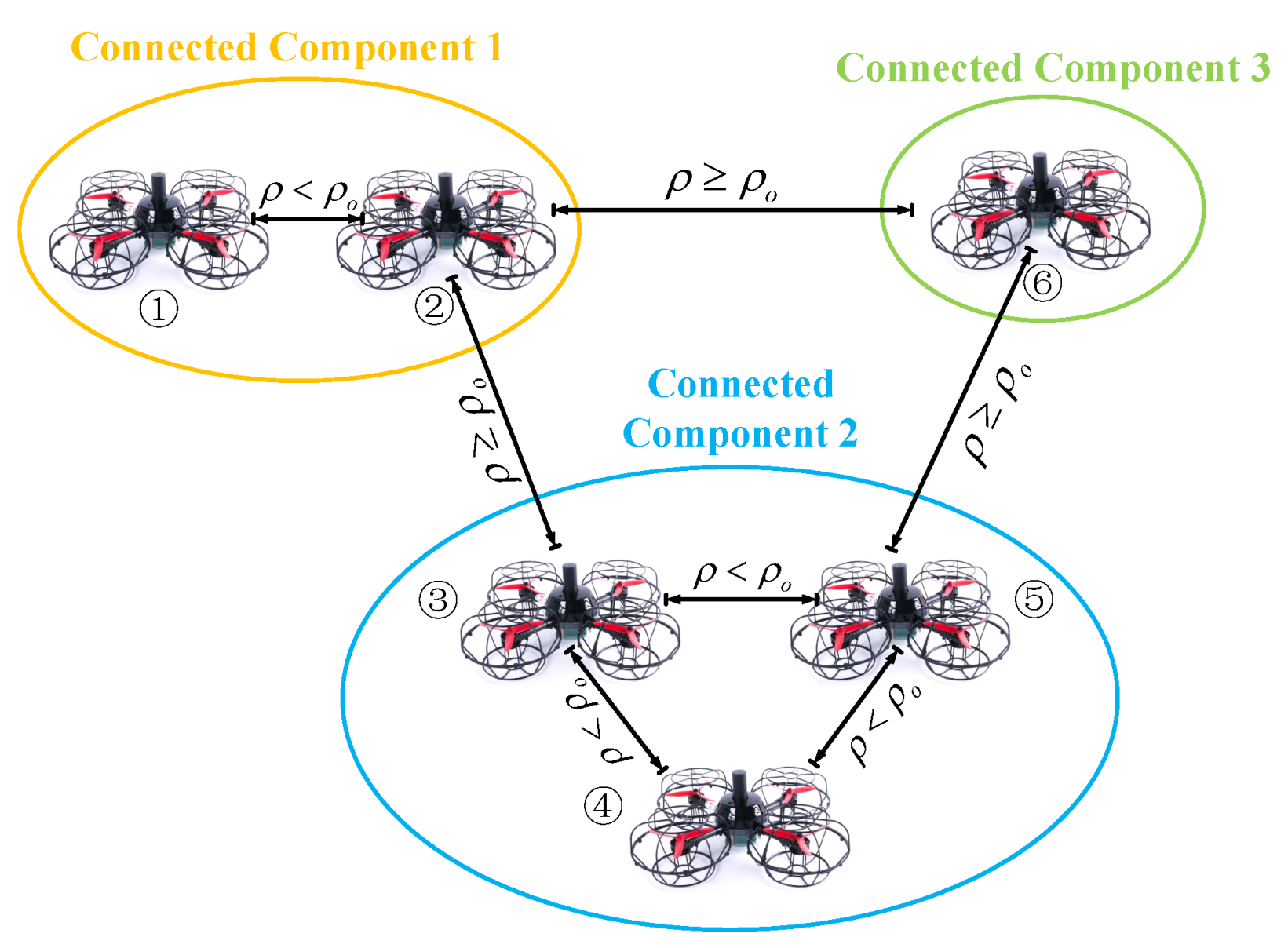
The communication topology between UAVs during formation transformation can be represented by an undirected graph $G=\{V,E\}$, where $V=\{v_1,v_2,\dots ,v_N\}$ is the set of UAVs and $E\subseteq V\times V$ is the set of edges representing the adjacent relationship among UAVs, i.e., edges $e_{ij}=(i,j)$ and $e_{ji}=(j,i)$ exist if the distance between the i-th UAV and the j-th UAV is less than ${\rho }_0$. The adjacent matrix $A\triangleq {\left[a_{ij}\right]}_{N\times N}$ contains elements $a_{ij}=1$, if there is an edge $e_{ij}$. A path between the i-th UAV and the j-th UAV is a sequence of edges $(i,j_1),(j_2,j_3),\dots ,(j_l,j)$. The graph G is said to be connected if there is a path for each pair of UAVs. A connected component is a subset of the graph which is associated with the smallest partition of the set of UAVs, and each partition is connected. Note that a disconnected graph has more than one component.

2.3.2. Dynamic Formation Transformation Algorithm

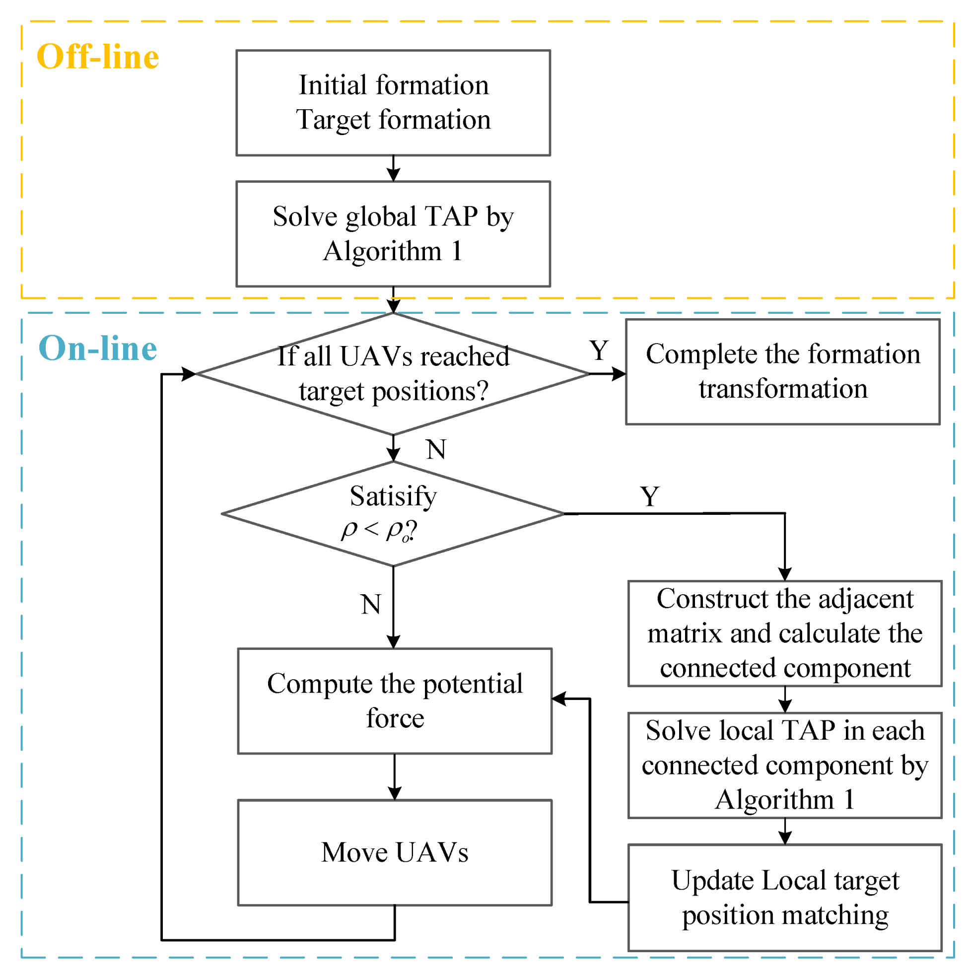
The Hungarian algorithm minimizes the total flight distance of all UAVs. One of the limitations of the Hungarian algorithm is that the minimum flight distance is obtained by statically considering straight lines between the initial and the target formations. However, UAVs deviate from such straight-line trajectory when avoiding collisions, thus may result in longer flight distance if the task assignment result remains the same. To address this issue, we propose a dynamic formation transformation algorithm by solving the TAP in a conditional-triggering manner during real-time trajectory planning using APF, as shown in Figure 2. To avoid heavy computational cost, a global TAP is first solved off-line and local TAPs are then formulated and solved on-line based on latest formation information.

Specifically, for each formation transformation (in general, a UAVs-LS animation contains a series of formation transformations), a global TAP in the form of (6) is firstly formulated off-line, seeking a match between the initial and the target formation coordinates of all UAVs, which includes

$$\begin{array}{cc}\hfill & {\mathbf{X}}_g={[{{\mathbf{x}}_{g,1}}^{\top },{{\mathbf{x}}_{g,2}}^{\top },\dots ,{{\mathbf{x}}_{g,N_g}}^{\top }]}^{\top },\hfill \end{array}$$

(13)

$$\begin{array}{cc}\hfill & {\mathbf{T}}_g={[{{\mathbf{t}}_{g,1}}^{\top },{{\mathbf{t}}_{g,2}}^{\top },\dots ,{{\mathbf{t}}_{g,N_g}}^{\top }]}^{\top },\hfill \end{array}$$

(14)

where ${\mathbf{X}}_g$ represents the current formation position coordinates and ${\mathbf{T}}_g$ represents the target formation position coordinates. $N_g$ is the total number of UAVs. The optimal match ${\phi }_g^{*}$ is obtained by using Algorithm 1 to solve the global TAP. A global APF is constructed by attracting UAVs to move along its negative gradient direction towards the target formation. During on-line operation, local repulsion fields are generated by the UAVs within a component.

When UAVs are moving in the air, the members of each component and the number of components may vary. The target position appointed by the current TAP may thus be affected in a component due to deviation from the original straight trajectory to avoid collisions. Therefore, a local TAP based on a conditional-triggering manner must be formulated and solved. In particular, the local TAP is triggered when there is a component. The connected components of undirected graph can be obtained by the adjacent matrix $A_{N\times N}$ [18,19]. An improved version of depth-first search has been proposed to solve the connected components in [19], and the method is employed to obtain the connected components of undirected graph. An illustrative example is given in Figure 3, where three components are formulated for six UAVs according to the adjacent relationship given in

Table 1. Adjacent relationship among six UAVs. UAV 6 has no adjacent UAV.

	UAV 1	UAV 2	UAV 3	UAV 4	UAV 5	UAV 6
Adjacent UAV No.	2	1	(4,5)	(3,5)	(3,4)	×

.

Table 2. Connected component solutions.

Connected Component No.	1	2	3
UAV No.	(1,2)	(3,4,5)	6

presents the solutions of the connected components.

Given a component $k,k=1,2,\dots ,m$ and its UAVs, we define the local TAP matching objectives ${\mathbf{X}}_l^k$ and ${\mathbf{T}}_l^k$ as:

$$\begin{array}{cc}\hfill & {\mathbf{X}}_l^k={[{{\mathbf{x}}_{l,1}^k}^{\top },{{\mathbf{x}}_{l,2}^k}^{\top },\dots ,{{\mathbf{x}}_{l,N_k}^k}^{\top }]}^{\top },\hfill \end{array}$$

(15)

$$\begin{array}{cc}\hfill & {\mathbf{T}}_l^k={[{{\mathbf{t}}_{l,1}^k}^{\top },{{\mathbf{t}}_{l,2}^k}^{\top },\dots ,{{\mathbf{t}}_{l,N_k}^k}^{\top }]}^{\top }.\hfill \end{array}$$

(16)

where ${\mathbf{X}}_l^k$ and ${\mathbf{T}}_l^k$ are the current and assigned target position of the k-th component. The local TAP solves the matching relationship between the current positions and target positions of the neighboring UAVs at discrete sampling instants while they are moving. Minimum flight distance can be maintained by using Algorithm 1 to solve the local TAP.

Consequently, a UAV-LS formation transformation (UAVs-LSFT) method is developed by combining the Hungarian algorithm and the APF dynamically, as summarized in Algorithm 2, which is simple enough for real-time computations.

Algorithm 2 Dynamic UAV-LS formation transformation algorithm

Input: initial formation $\mathbf{X}$, target formation $\mathbf{T}$ 1: Obtain the global optimal assignment by Algorithm 1 2: while at each sampling instant do 3:     if $\rho <{\rho }_0$ then 4:         Construct the adjacent matrix A 5:         Compute the connected components by [19] 6:         Obtain the local optimal assignment by Algorithm 1 7:         for each UAV do 8:            Compute the resultant force by (12) 9:            Obtain the next way-point 10:         end for 11:     else 12:         for each UAV do 13:            Compute the resultant force by (12) 14:            Obtain the next way-point 15:         end for 16:     end if 17:     if all the UAVs have reached the target position then 18:         Stop 19:     end if 20: end while

3. Software Platforms

In the UAV-LS system, two software applications are developed using C# to provide animation design and real-time monitoring functionalities. The work flow of the two applications is shown in Figure 4.

3.1. Animation Design Interface

In the ADI, the coordinates of UAVs representing specific formations can be designed by users. The two main functions of the ADI are the formation drawing and the flight mission simulation.

First, the longitude $Lo{n}^0$ and latitude $La{t}^0$ of each UAV is determined in the formation drawing function by drawing a bitmap or by Photoshop design bitmap, as shown in Figure 6a, where each dot represents the center of a UAV. The horizontal direction is set as the x-axis and the vertical direction as the y-axis in the bitmap. In addition, the height of the UAVs and the tilt angle along the x-axis or y-axis can be configured. In this function, the global TAP is solved off-line to obtain the optimal match based on the coordinates of the initial and target formations when the drawing is completed. The interface converts the coordinates of UAVs into way-point positions, which are saved into a text file for simulation and real-time control.

The way-point information structure is shown in Figure 5, where R, G, and B, respectively, represent the red, green, and blue of the three primary colors which are used to control the light color of the UAV LED module. T is used to indicate the maintenance time of the formation, and only plays a role in the automatic execution mode of the formation control. Lon, Lat, H, respectively, represent the longitude, latitude, and relative ground height of the target point. Specifically, Lon and Lat can be calculated by

$$\begin{array}{cc}\hfill Lon& =Lo{n}^0+{\displaystyle \frac{x_{Lon}}{△Lon}}\hfill \end{array}$$

(17)

$$\begin{array}{cc}\hfill Lat& =La{t}^0+{\displaystyle \frac{y_{Lat}}{△Lat}}\hfill \end{array}$$

(18)

where $△Lon$ is the longitudinal distance change in meters when the longitude changes by one degree under the same latitude. Similarly, $△Lat$ is the latitudinal distance change. It should be noted that the influence of the curvature of the earth is ignored in (13) and (14), since the entire UAV-LS area is small enough to be regarded as a plane.

Second, the saved way-point information is loaded in the flight mission simulation function. The function is designed to simulate the UAVs-LS graphics in a virtual environment as shown in Figure 6b. To simplify the simulation process, each UAV moves to the target point in a straight line at the same speed. The user can view the simulation process from any perspective to examine the performance of the UAVs-LS.

3.2. Real-Time Monitoring and Control Interface

In the real-time monitoring and control interface, specific UAV formation control commands can be sent from the GCS to the UAVs. Common commands range from managing functions such as connecting, receiving way-points, and sending data, to control functions such as collective/sequential takeoff, autonomous control, and collective/sequential landing. As shown in Figure 7, the status of UAVs is displayed in the interface and common control commands that are programmed a priori can be sent by one click. More complex commands are also supported for users with programming skills. During the UAV-LS, the hybrid formation transformation algorithm is periodically performed in real time to generate collision-free reference trajectories based on the latest UAV status and the target way-point information.

4. Hardware Setup

4.1. Quadrotor Prototype

Quadrotors are often chosen as basic aerial robot research platforms due to their low price and flexibility in design and assembly. In this paper, quadrotors are made up of three parts, i.e., an ellipsoidal control center, a carbon fibre frame, and four rotor units. The control center accommodates an onboard control unit, a duplex wireless communication module, a positioning unit, a rechargeable lithium battery, and an LED module. The battery pack is placed at the center of the quadrotor to improve the horizontal stability. The LED module, set at the bottom of the quadrotor and protected by a transparent polyvinyl chloride shell, produces 16.78 million colors of light at night. Four rotor units of the quadrotor are composed of brushless direct current (BLDC) motor and three-blade propeller. The carbon fibre frame connects the rotor units with the controller center. The quadrotor is shown in Figure 8, with a 24.5 cm diagonal wheelbase, 16 min maximum hover time, 3S 3300 mAh lithium battery and 0.6 kg weight.

4.2. High Accuracy Positioning System

In general, quadrotors make use of GPS and inertial measurement unit (IMU) system for positioning [20,21]. However, GPS and IMU are not suitable for high-accuracy applications for two reasons: (1) GPS positioning accuracy is sensitive to atmospheric (ionosphere and troposphere) delay, ephemeris error, clock bias, and multi-path effects; (2) The choice of IMU is limited by the weight and size of UAVs. In this paper, the real-time kinematic GPS (RTK-GPS) system is employed. The RTK-GPS uses carrier phase as correction data to eliminate atmospheric delay of GPS which is the main source of the time error, resulting in centimeter-level positioning accuracy [22].

The RTK-GPS has three parts, i.e., rover station, base station, and GCS connected to a wireless router. The RTK-GPS base station consists of a GPS antenna, a GPS receiver, and a stream server. The GPS receiver outputs raw positioning observation data, including satellite ephemeris, pseudorange, integrated carrier phase, and Doppler shift. The stream server converts the raw observation data into correction data in RTCM format. Then, the correction data are sent from the stream server to GCS. The GCS, connected to a wireless router, broadcasts the RTCM correction data to UAVs. The RTK-GPS rover unit in the quadrotor is composed of an GPS antenna, a GPS receiver, and a position solver board. The position solver board obtains the correction data of the base station through wireless communication with GCS and the observation data from the on-board GPS receiver, and produces the high accuracy real-time position of the rover antenna by the RTK-GPS library (RTKLIB) positioning algorithm [23].

4.3. UAVs-LS System Setup

As shown in Figure 9, the UAV-LS system consists of a decision-making sub-system, a RTK-GPS positioning sub-system, a wireless communication sub-system, and a UAV sub-system. Specifically, sensor information is sent from UAVs to the GCS through a wireless communication subsystem periodically. The information includes precise latitude and longitude coordinates obtained by the RTK-GPS positioning unit and the relative ground height provided by the barometer. Since UAVs and GCS are two different platforms running different operating systems, the interactive message exchange is enabled by using the MAVLink protocol [24]. At the GCS, a series of decisions are made and collision-free trajectories are planned, which are sent to the UAVs through the wireless communication. The autopilot controller on UAVs adjusts UAV locomotion modes to track the reference trajectories.

5. Simulation and Experiment Results

In the section, we first present the comparison and analysis between the proposed dynamic formation transformation method and another two methods. Then outdoors experiments using six quadrotors are performed.

5.1. Simulation

Three methods are compared in the simulation. Method 1 is the traditional method which separates the task assignment and trajectory planning, i.e., task assignment is performed offline only before the formation transformation. Method 2* is the proposed dynamic formation transformation algorithm where a global TAP is solved offline once and local TAPs are formulated and solved in connected components online. Method 3 sets as a benchmark where global TAPs are solved online once collision avoidance movement occurs.

The simulations consider a three-dimensional environment with the length, width, and height of $50\times 50\times 50$ m. The initial and target states in the formation are randomly generated. The attractive gain coefficient $\eta$ is set to 0.8, and the repulsive gain coefficient $k_p$ is set to 0.3. The influence radius of repulsion point ${\rho }_o$ is set to $2.3$ m. The sampling time is 20 ms. A UAV is considered to have arrived at its target when the distance between them is less than 0.01 m.

The simulation platform is MATLAB2020a running on a PC with AMD 3970X. It should be noted that only a single CPU core is utilized. The simulation is repeated 100 times in which the initial and target positions of the UAVs are randomly generated. For a fair comparison, the initial and target positions are the same for three methods in each test. The average computation time for each iteration, the average flight distance of the UAVs arrived at the target position, the maximum distance moved among the UAVs, the time taken for all UAVs to reach their targets and the number of the UAVs reached the destination are shown in

Table 3. Comparison of simulation results of the formation transformation of 600 UAVs using three methods.

	Method 1	Method 2*	Method 3
Computation time (ms)	9.55	13.8	21.6
Flight distance (m)	4.8327	4.8132	4.8027
Maximum distance (m)	16.3102	14.3991	14.3725
Arrival time (s)	73.63	62.01	61.62
Arrived UAVs	565.97	566.64	566.67

.

It can be seen that Method 1 has the shortest average computation time because the TAP is solved only once. The proposed Method 2* has a slightly longer computation time than Method 1 but it is far less than that of Method 3. However, the number of arrived UAVs for Method 2* and Method 3 is almost the same, and is larger than Method 1. The average flight distance and the maximum flight distance of Method 2* is slightly longer than Method 3 by only solving local TAPs in connected components, while Method 1 has the longest average flight distance and maximum fight distance since it solves a global TAP once offline without guaranteeing the optimality of the TAP during collision avoidance. Similarly, Method 1 has the longest arrival time, Method 2* and Method 3 are obviously lower than Method 1 which benefit from the TAP solution during the formation transformation. The targets of part of UAVs are updated after solving the TAP, and the flight distance is shortened so that all drones may transform the desired formation in a faster way. In conclusion, the proposed Method 2* achieves a good trade-off between performance and efficiency. Method 2* is better than the traditional static Method 1 in terms of flight distance, arrival time and arrived UAVs, and is also computationally efficient when compared to the global optimal Method 3.

Remark 1.

The initial and target positions of the UAVs are uniformly randomly generated in the simulation. While most UAVs are allocated to nearby targets with a straight-line trajectory, a small number of UAVs need to avoid inter-collisions hence deviate from the straight-line trajectories. Since the flight distance of the three methods is averaged in Table 3, the distance differences among the three methods seem small. However, the benefit of dynamically solving TAP cannot be ignored, especially in denser and more compact spaces, and for reducing the arriving time of UAVs.

Remark 2.

Due to the randomness of the initial and target position, the distance between some target points are less than the safe distance. This makes it impossible for the UAVs to arrive at the destination. Moreover, a few UAVs were trapped into extreme point due to the repulsive force of multiple UAVs, which also causes the inability to reach the target position. Therefore, all three methods cannot guarantee that all UAVs arrive at their target positions. To solve this issue, the minimum distance between generated target positions can be configured in the formation transformation to increase the number of UAVs arriving at the target positions. In addition, using Method 2* and Method 3 can reduce the influence of extreme points on the number of arrived UAVs, which is an advantage of our proposed method.

Remark 3.

In the simulation, conservative attractive and repulsion coefficients are selected in a compact space with a large number of UAVs generated randomly, for finding a balance between sampling time and smooth trajectories. As a result, the UAVs take a relatively long time (about 60s) to arrive at their targets. Nevertheless, the attraction and repulsion coefficients can be tuned according to UAV specifications and the flight space to reduce the arriving time.

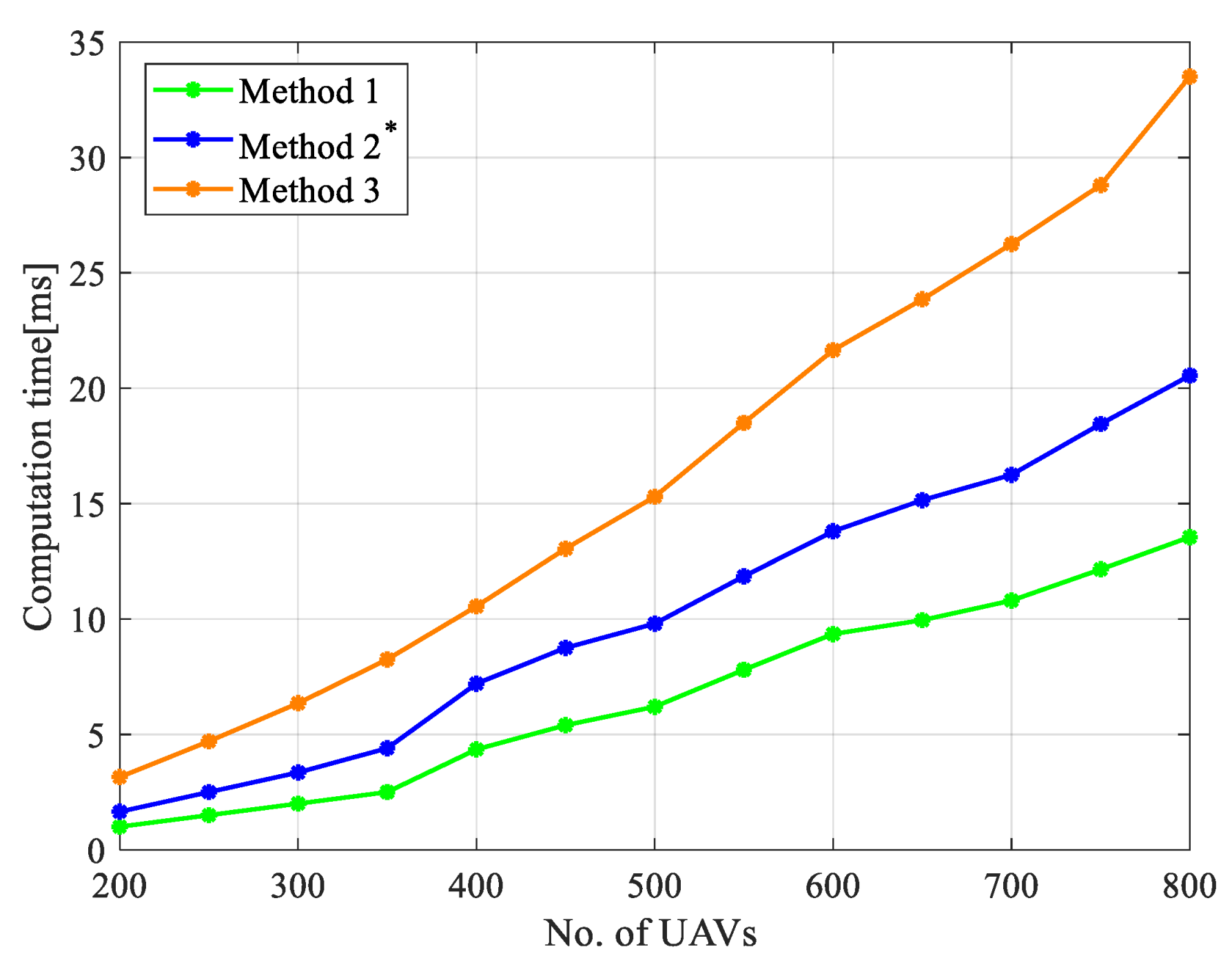
To further understand how the number of UAVs affects computational time, we set the number of UAVs as a single variable, the average computation time for each iteration is shown in Figure 10. Compared with Method 3, the proposed method has a significant computational cost advantage, and the advantage becomes more obvious as the number of UAVs increases.

Next, two case studies are given to better demonstrate the advantages of the proposed method in fight distance and the number of arrived UAVs. The trajectory of using Method 3 is not shown since it is indistinguishable from that of the Method 2*. In these case studies, the attractive gain coefficient is $\eta =0.8$; the repulsive gain coefficient $k_p$ is $0.3$, and the other parameters are kept the same.

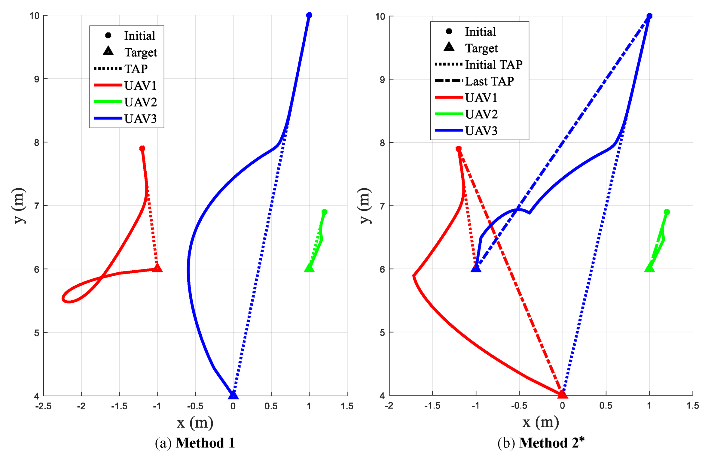
5.1.1. Case A

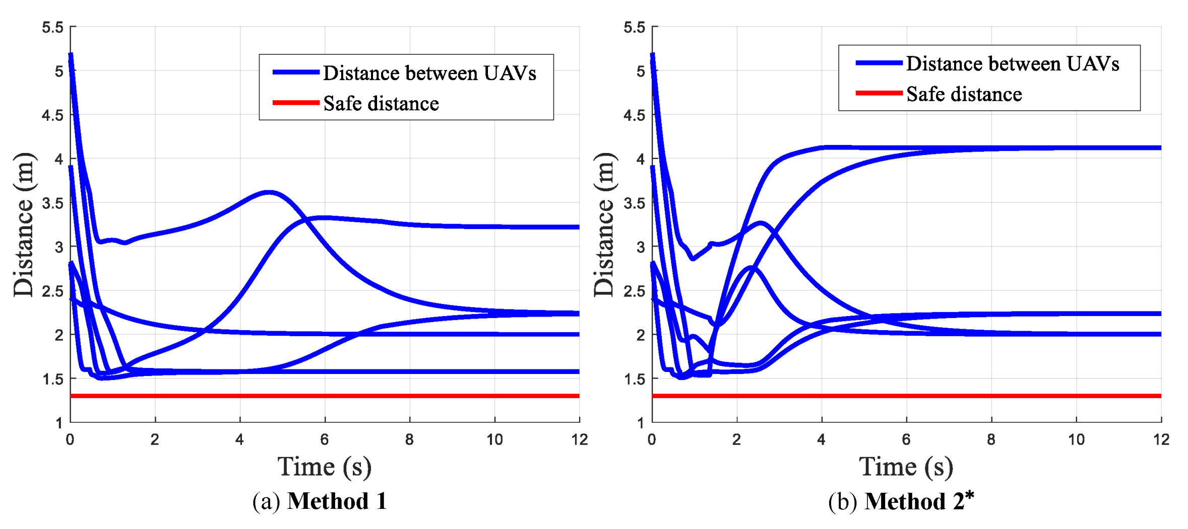
In Case A, three UAVs realize formation transformation using Method 1 and Method 2*. The initial positions of the three UAVs are ${\mathbf{x}}_1=[-1.2;3.9;6]$, ${\mathbf{x}}_2=[1.2;2.9;6]$, and ${\mathbf{x}}_3=[1;6;6]$. The positions of the target formation are ${\mathbf{t}}_1=[0;0;6]$, ${\mathbf{t}}_2=[-1;2;6]$, and ${\mathbf{t}}_3=[1;2;6]$. The trajectories of UAVs are displayed in Figure 11 and the distance between the UAVs is given in Figure 12.

It can be seen from Figure 11 that all UAVs arrived at their offline assigned targets using Method 1, despite the significant deviations from the planned straight-line trajectory. Using Method 2*, local TAPs are solved online such that UAV 1 and UAV 3 are assigned to different targets while avoiding collisions. The flight distances of the three UAVs are shown in

Table 4. Flight distance (m) of the three UAVs in the formation transformation process.

Variable	UAV 1	UAV 2	UAV 3	Average	Arrival Time (s)
Method 1 (m)	4.2540	0.9339	6.5813	3.9231	45.7
Method 2* (m)	4.7485	0.9340	4.8313	3.5046 (−11%)	38.8 (−15%)

. Compared with Method 1, the average flight distance and the arrival time of Method 2* are reduced up to $11\%$ and $15\%$, respectively. Both methods can maintain the safe distance among UAVs during the formation transformation.

5.1.2. Case B

In Case B, four UAVs are simulated to construct a desired formation, where the initial positions are ${\mathbf{x}}_1=[-1.2;3.2;6]$, ${\mathbf{x}}_2=[1.2;2.9;6]$, ${\mathbf{x}}_3=[0.8;8;6]$ and ${\mathbf{x}}_4=[-1.2;6;6]$. The positions of the target formation are ${\mathbf{t}}_1=[-1;2;6]$, ${\mathbf{t}}_2=[1;2;6]$, ${\mathbf{t}}_3=[0;0;6]$, and ${\mathbf{t}}_4=[0;-2;6]$. The trajectories of the four UAVs and the distance between the UAVs are shown in Figure 13 and Figure 14, respectively.

Using Method 1, UAV 4 stops at a local minimum and is unable to arrive at the target, as shown in Figure 13a. In Figure 13b, local TAPs are triggered on and solved during collision-avoidance. All four UAVs have arrived at the target. The flight distance of the UAVs is shown in

Table 5. Flight distance [m] of the four UAVs in the formation transformation process.

Variable	UAV 1	UAV 2	UAV 3	UAV 4	Average	Arrival Time (s)
Method 1	1.2555	0.9266	10.4624	×	4.2148	61.6
Method 2*	1.2555	5.0480	7.2017	6.7763	5.0704	40.7 (−34%)

. It can be seen that using Method 2* increases the flight distance in this case, yet the number of UAVs that can arrive at the target position is increased and the arrival time is reduced up to $34\%$. The proposed dynamic task assignment and trajectory planning algorithm successfully helps UAVs escape from the local minimum point.

5.2. Experiment

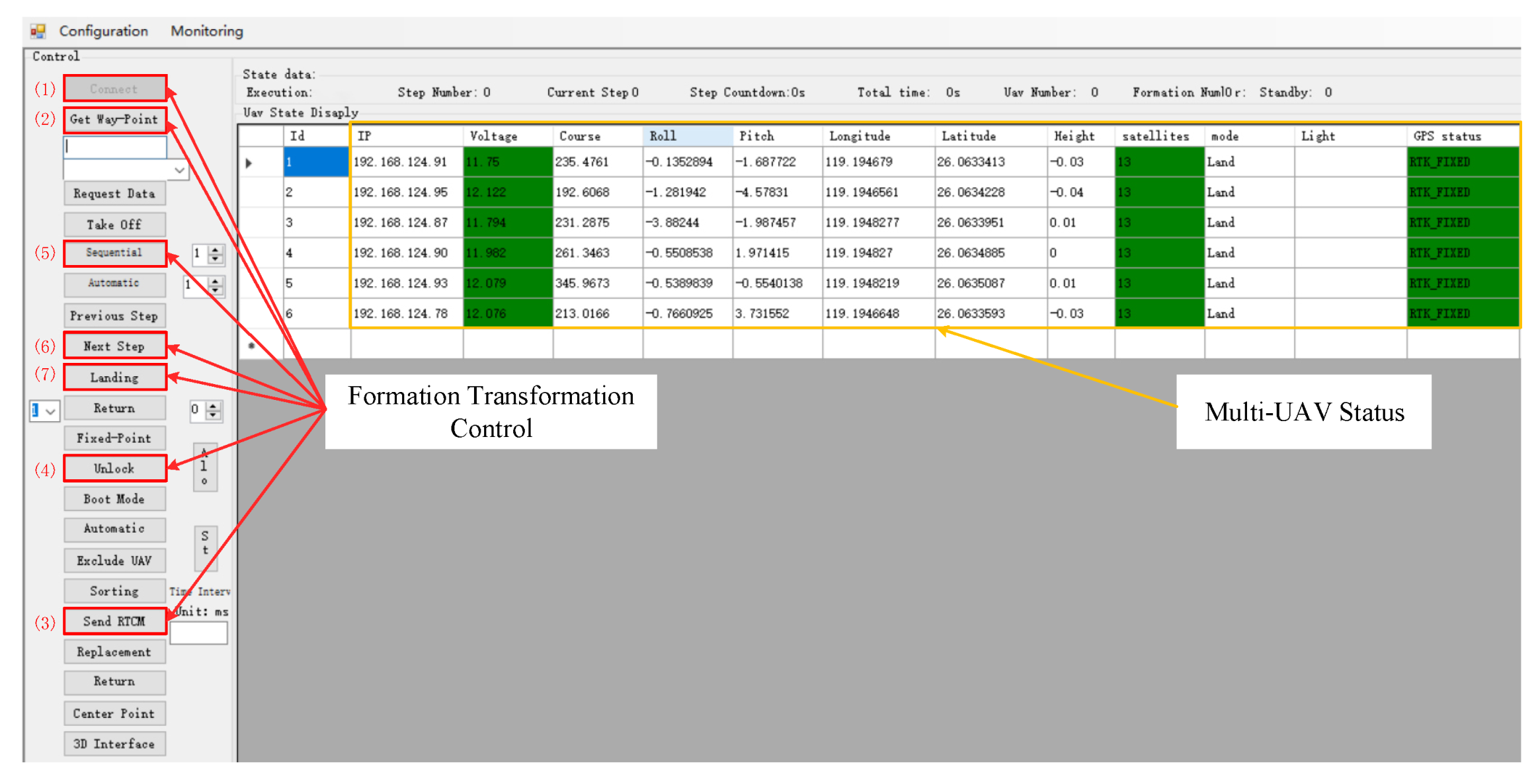
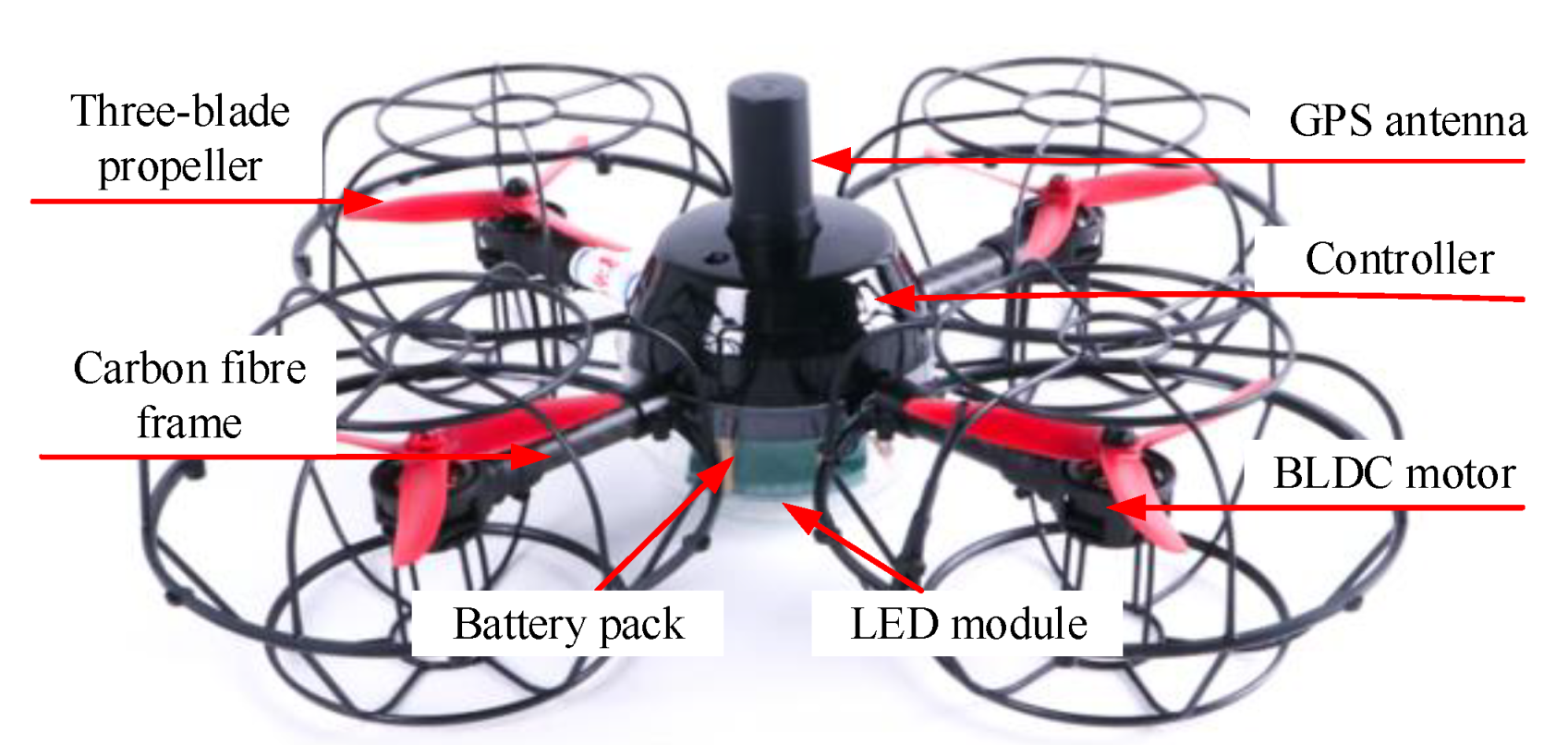
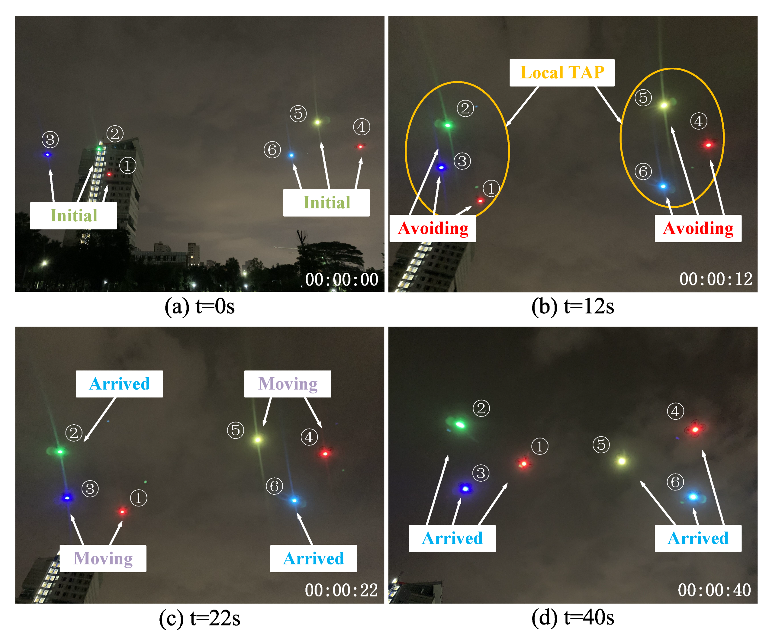
In this work, an experiment with UAV-LS is carried out consisting of 6 quadrotors transformed from a random initial formation to a desired formation. A laptop equipped with i7-7700hq CPU and 8GB RAM is used as the GCS for animation design, simulation, and real-time monitoring and control.

Real-time measurement data are sent from UAVs to the GCS at a frequency of 10 HZ and the collision-free reference trajectories are planned by the proposed dynamic formation transformation algorithm, which is sent back from the GCS to the UAVs at a frequency of 5HZ. The attractive gain coefficient $\eta$ is set to 0.8, and the repulsive gain coefficient $k_p$ is set to 0.3. The influence radius ${\rho }_o$ of other UAVs is set to 2 m.

In this experiment, the multi-threaded programming feature of C# is used. The GCS computer has 4 cores and 8 threads, in which 6 threads are enabled, each of which computes reference trajectories for a quadrotor in parallel. The initial and target formation positions of the quadrotors are given in

Table 6. Coordinates of the initial and target formations.

Initial states X of the UAVs
Variable	UAV 1	UAV 2	UAV 3	UAV 4	UAV 5	UAV 6
x(m)	1.2	−1.2	−1	−1.2	1.2	1
y(m)	5.4	4.4	7.5	−4.9	−3.9	−7
z(m)	6	6	6	6	6	6
Target formation states $\mathbf{T}$
x(m)	0	1	−1	0	−1	1
y(m)	1.5	3.5	3.5	−1	−3	−3
z(m)	6	6	6	6	6	6

.

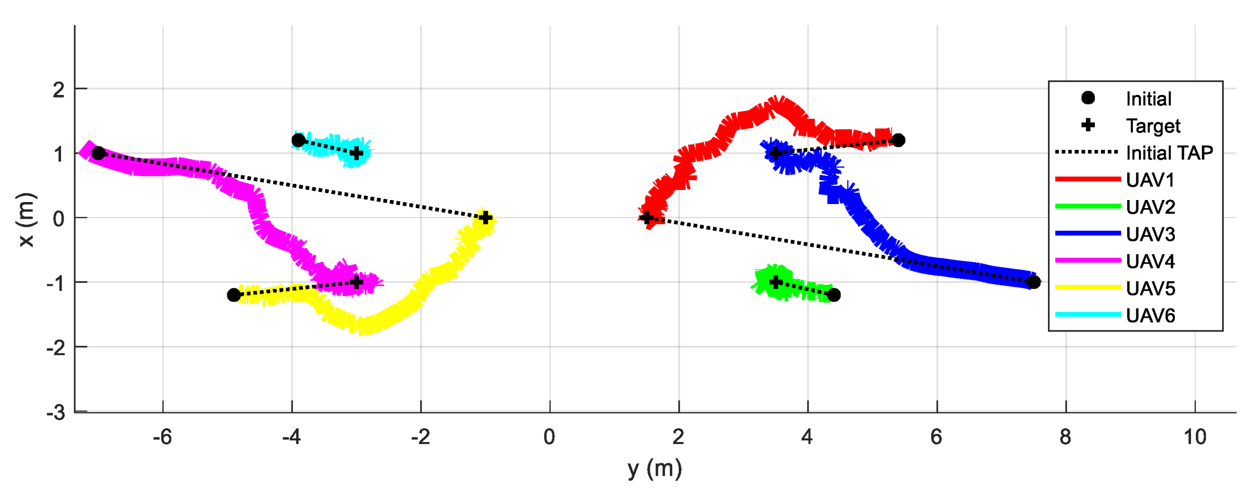
Onsite photos of the UAV-LS at times 0, 14, 22, 40 s are shown in Figure 15, where (a) shows all quadrotors are steadily waiting at the initial formation; (b) shows all quadrotors started to avoid collisions and the local TAPs are solved in two connected components, which are formed by the 1st, 2nd, 3rd UAV and the 4th, 5th, 6th UAV, respectively; (c) shows the 1st, 3rd, 4th and 5th UAV are moving to the target way-points; and (d) all quadrotors have arrived at their targets. Figure 16 presents the actual trajectories of the 6 quadrotors on the X–Y plane during the experiment. Figure 17 illustrates the minimum distance of each quadrotor from the others during the formation transformation. It can be concluded that the proposed task assignment and trajectory planning algorithm are able to dynamically plan the trajectories of UAVs when they deviate from the initial trajectory due to collision avoidance. The safe distance is always maintained during the experiment.

5.3. Discussion

In Section 5.1, comparative simulation experiments were carried out among the three methods. Compared with Method 1 which decouples task assignment and trajectory planning, the proposed Method 2* has advantages in terms of shorter flight distance, shorter arrival time and more arrived number of UAVs. The disadvantage compared with Method 1 is the increased computational time. Compared with the Method 3 which solves a global TAP once collision avoidance movement occurs, the proposed Method 2* has slight disadvantages in flight distance, arrival time, and number of arrived UAVs. Yet, the proposed Method 2* has obvious advantages over Method 3 in terms of computational time and the scalability, as shown in Figure 10. In Section 5.2, an experiment with UAV-LS successfully verified the effectiveness of the proposed method in practice.

Through the above analysis, the proposed method achieves a good trade-off between performance and efficiency which is desired for most multi-UAV systems with a number of controlled UAVs and limited computing resources.

6. Conclusions and Future Work

In this paper, a UAV-LS system is developed including a dynamic task assignment and trajectory planning algorithm, a software toolkit and hardware design and realization. In particular, the dynamic formation transformation algorithm works in a conditional-triggering manner where local TAPs of connected components are constructed and solved online to achieve minimum flight distance and to reduce the impact of collision avoidance on task assignment. To build such a UAV-LS system, a wireless transmission subsystem was established to transfer data based on the MAVLink protocol between the UAVs and the GCS, and the RTK-GPS technique was utilized to provide centimeter-level positioning accuracy for UAV. Simulations and experiments were conducted to verify the proposed UAV-LS system.

In future work, efforts will be devoted to cooperative formation transformation techniques. Flight distance balancing issues will also be considered, i.e., the difference between the flight distance of each UAV is minimized to avoid battery energy imbalance.