The Use of Transfer Learning for Activity Recognition in Instances of Heterogeneous Sensing

Abstract

Transfer learning is a growing field that can address the variability of activity recognition problems by reusing the knowledge from previous experiences to recognise activities from different conditions, resulting in the leveraging of resources such as training and labelling efforts. Although integrating ubiquitous sensing technology and transfer learning seem promising, there are some research opportunities that, if addressed, could accelerate the development of activity recognition. This paper presents TL-FmRADLs; a framework that converges the feature fusion strategy with a teacher/learner approach over the active learning technique to automatise the self-training process of the learner models. Evaluation TL-FmRADLs is conducted over InSync; an open access dataset introduced for the first time in this paper. Results show promising effects towards mitigating the insufficiency of labelled data available by enabling the learner model to outperform the teacher’s performance.

1. Introduction

Activity recognition (AR) is a research area focused on identifying human actions from a collection of sensor data. Often, solutions rely on design-time techniques that remain static after being trained once and assume that further data derives from identical sources and conditions. However, real-world applications require solutions to embrace the unpredictability of daily living and allow for exposure to unexpected changes. A practical alternative is required to address these issues, and transfer learning, if carried out successfully, can significantly improve the performance of AR data-driven modelling.

Transfer learning is inspired by the capabilities of humans to transfer knowledge across tasks, where the knowledge from one domain can improve the learning performance or minimise the number of labelled samples required in another domain. It is of particular significance when tackling tasks with limited labelled samples. Within AR, transfer learning is an approach in which previous knowledge or a previous process addresses a new, but related, task [1,2]. It accomplishes this by reusing the existing learned patterns on a source domain to identify the similarities within tasks, regardless of the environment or technological setting in a target domain. Hence, while conventional solutions to address AR problems rely on machine-learning approaches, the benefits of reusing existing knowledge can positively impact the training time of machine-learning algorithms.

Transfer learning techniques have proved their wide applicability to the automatic learning and recognising of activities from scenarios where training data is already available in the source domain, enabling the transfer of knowledge to different technologies, subjects, and settings at run-time. These techniques are being used as a starting point for training classification machine-learning models, such as in a convolutional neural network (CNN) that allows classification models to reduce the training investment. In particular, researchers have employed transfer learning to extend the features extraction when training machine-learning classifiers [3]. Two of the attributes commonly investigated for CNNs are architectures [4] and fine-tuning [5], where researchers use already trained CNN architectures and extend them by incorporating new convolutional layers to fine-tune the machine-learning models. Although these strategies are common in scenarios where the feature-distribution is similar between domains, other techniques, such as teacher/learner (T/L), active learning (AL) and fusion techniques denote an alternative to address problems where the feature-distribution is different [6].

Problem Statement and Contribution

The underlined problems are that while transfer learning offers a mechanism to leverage small labelled datasets, current research efforts are restricted to sensing technology, which relies on a similar feature-space. Simultaneously, current alternatives tend to be impractical due to the inconvenient method of labelling intervention that increases the time and resources costs, as well as the effort investment.

T/L modelling presents a new perspective on transfer learning that enables the transferability of knowledge in scenarios where the feature-space is different; however, it introduces some challenges. A major challenge is that the accuracy of the teacher limits the accuracy of the Learner, as the system’s only source of a ground truth comes from the teacher, and, thus, the learner is entirely reliant upon the teacher. Hence, it remains to be explored whether the Learner can outperform the teacher.

This problem presents the opportunity to investigate the benefit of MWE sensing technology and, together with its sensing characteristics, to train a classification model underlined by transfer learning techniques to mitigate the insufficiency of labelled data for ADL problems when the feature-space is different.

The key contributions of this paper are two:

• TL-FmRADLs: a framework that integrates the T/L, AL and data fusion techniques that offers to optimise the performance of learner AR models regardless of the sensing technology source;
• InSync: an open-access dataset that consists of subjects performing activities of daily living while data are collected using three different sensing technologies to facilitate the community future research in transfer learning.

The rest of the paper is organised as follows. The next Section 2 presents the background of the T/L, AL, and fusion techniques in a broader sense to build the foundations and scope of our investigation. Then, in Section 3 we introduce TL-FmRADLs and explain its different algorithms in the subsequent sub-sections. The experiment setup is presented in Section 4, followed by the introduction of InSync Dataset in Section 5. Section 6 presents implementation details. Results and Discussion are presented in Section 7 and Section 8, respectively. In the penultimate Section 9, we highlight research issues and potential future directions, whereas the final Section 10 presents the concluding remarks of this paper.

2. Preliminaries

Whereas there are different kinds of knowledge representation investigated within transfer learning such as instance-transfer [7], feature-representation-transfer [8], parameter-transfer [9] and relational-knowledge-transfer [10], as discussed in detail in our previous work [1]. This paper builds upon one of the findings reported by Hernandez et al. [1], who observed that the T/L technique is a niche owing to its novelty, and stated that along with the potential of transfer learning techniques within the area of AR to mitigate the insufficiency of labelled sensing data, transfer learning has been shown to be progressing when using the same sensing technology, i.e., feature-space and dimension. However, there has been little work completed on transfer knowledge between any two or more sensor modalities. In this regard, some authors proposed leveraging the capabilities across sensing technologies, focused on fusion techniques [11,12,13,14,15], while other authors suggested using a T/L model.

2.1. Teacher/Learner

T/L is a technique in which no training data are required; instead, a previously-trained classifier model (teacher) is introduced to operate simultaneously with a new classifier model to be trained (learner) and provides the labels for the observed data instances; this enables the capabilities of a Learner to perform AR utilising a teacher regardless of the sensor data the teacher was trained with. T/L modelling for AR has shown to have significant potential for improving transfer learning to make systems more robust and versatile [6,16,17,18,19,20,21].

Some researchers have investigated T/L; for example Rokni and Ghasemzadeh [17], Kurz et al. [18] and Roggen et al. [19] presented alternatives to enable the transference of knowledge, where labelled data are fully available in the source data, but only a fraction of the data are available in the target domain. Overall, the approach consists of incrementally training the model on the target data. The limitation of these studies, however, lies in the assumption that both the source and the target data consist of the same feature-space. Hu and Yang [22] and Zheng et al. [23] have proposed alternatives that relax the assumption of the same feature-space by transferring knowledge across different activities and different sensors. They built a mapping between the source and the target domains over a bridge built upon web knowledge. Although their experimentation consisted of different data in highly different-spaces, their extension to mobile, wearable, and environmental (MWE) sensing devices is uncertain. Fallahzadeh and Ghasemzadeh [24] proposed an uninformed algorithm that leveraged the similarities by constructing a deep neural network (DNN) based feature-level representation of the data in the source and the target domain. The algorithm uses a heuristic classifier-based mapping to assign activity labels to the core observations. Finally, the output of the labelling is fused with the prediction of the source-model to develop a personalised AR algorithm. The limitation of this study, however, lies in the constraint that it relies on the same feature-space. One general limitation of T/L approaches, however, is that the accuracy of the learner’s training is bounded by the accuracy of the teacher.

2.2. Active Learning

AL is a technique that seeks to achieve increased accuracy with fewer instances of labelled data by being able to question the training data from which to learn selectively. Unlike traditional machine-learning, AL can update a system as part of a continuous and interactive learning process to annotate unlabelled data [25,26,27].

Some research has shown the feasibility of this technique. For example, Hu et al. [28] proposed a method that self-supervised incremental learning knowledge that received contextual information to gradually personalise models for individual subjects. Saeedi et al. [29] introduced an architecture that adapts a machine-learning model developed in a given context to a new setting or configuration, by learning from human annotators as experts. Dao et al. [30] proposed a new method with adaptive, interactive, general personal-model training components and data sharing on the cloud; the advantage of their approach was the fast adaptation on new subjects on its deployment and the opportunity to enhance predictability by other subjects being gradually integrated; this then helped to increase the accuracy of the model over iterative retraining.

Although the studies described above have shown feasibility in contributing to the solution of modelling problems for ADLs, their limitation, however, relies on one of the following cases: (i) AL assumes human annotation as a feedback source, which interrupts the user’s day-to-day activities, making those solutions less practical; or (ii) the approach ignores labelled data from overlapped models that could be used locally, as stated by the T/L approach. An approach to address the first problem is T/L, in which a teacher can enable the scalability of a system by acting as an oracle; for the second problem fusion techniques can be utilised, where fusion represents a technique that integrates multi-sensor data to enhance the inference of activities that could not be feasible from a single sensor [14,15,31].

2.3. Fusion Techniques

Fusion techniques combine data from multiple sensors to achieve improved accuracy and more specific inferences than can be achieved by the use of only a single sensor. They have been employed on multi-sensor environments with the aim of fusing and aggregating data from different sensors. The goal of using fusion in multi-sensor environments is to obtain a lower detection error probability and an improved reliability using data from multiple distributed sources [32].

Fusion techniques have shown to be effective in problems aligned with AR. For example, Song et al. [33] presented a method to enable dense embedding using kernel similarities. Junior et al. [34] proposed a classifier-fusion schema using learning algorithms, in which feature extractors and classifier combinations were used to achieve higher accuracy. Nweke et al. [35] presented a comparison of the performance achieved by single- and multi-sensor fusion for AR using inertial data. The results of these studies showed the significant impact of multi-sensor fusion for recognising human activities, demonstrating the feasibility of fusion techniques for addressing AR problems.

3. Transfer Learning Framework for Recognising Activities of Daily Living across Sensing Technology

TL-FmRADLs offers to automatically optimise the performance of AR models regardless of the sensing technology source. To introduce TL-FmRADLs, Figure 1 shows its three key phases, namely, data preparation, transfer learning, and AL.

The first phase consists of preparing the sensor signal under a homogenised format to facilitate the manipulation of data regardless of the sensing technology. The second phase corresponds to the T/L approach to train untrained AR models (learner). Finally, the third phase updates the learner models over data feature fusion pulled from learner models. Details of these phases are presented next.

3.1. Teacher/Learner Phase

Similarly to the conventional machine-learning modelling’s process, TL-FmRADLs entails two stages, namely, training and testing. The training stage embraces all three phases of TL-FmRADLs (data preparation, transfer learning, and AL), whereas the testing stage embraces only phases 2 and 3 (transfer learning and AL).

Referring to the steps from phase 1 illustrated in Figure 1, raw data gathered from the available sensor devices are immediately pre-processed (1, 2). Data are then fragmented in small time-windows to capture fine gestures involved within the AR events (3).

As part of the second phase, the segmented data are sent to a front-desk ($FD$) component (4), which will then seek for a legacy version or else a compatible AR model based on a semantic-based search [36]. If the $FD$ finds a legacy version, the legacy version is assigned with a teacher role (5a); otherwise the model builder ($MB$) component builds the AR model upon any labelled data available at this step (5d). Another possible variation, however, is when the $FD$ finds more than one legacy AR model (5b), in which case the AR model with higher classification accuracy will emerge as teacher (5c).

Formalisation and Pseudo-Code

To further detail on the functionality of the different components introduced above, this Section first presents the primary algorithm corresponding to the T/L phase, followed by its derived dependencies/functions. As presented before and illustrated within steps from 5a to 5d from Figure 1, one of the responsibilities of the $FD$ component consists of assigning a T/L role to the incoming AR models. In Algorithm 1, we can observe that the $FD$ assigns roles based on the performance of the AR model given by $unseenActRate={\sum }_{k=1}^l\frac{D_S^{\prime }}{{D_S}_k}$, in which k is the kth AR model within a pool of AR trained models $D_{S[·]}$, and $D_S^{\prime }$ stands for a complementary AR trained model, where $D_S^{\prime }\in D_{S[·]}$ and $D_S^{\prime }\ne {D_S}_k$.

Although $unseenActRate$ consists of a scalar value that states the error loss retrieved from the function $setTrainingModel(·)$ the validation to determine the T/L roles is dictated by the function $getValidationUponRuleSchema(·)$ (detailed in Algorithm 2), in which the lower the ratio of unseen activities, the more chances to become a Teacher ($D_S$). To ensure selecting the proper teacher model, the $FD$ tests all associated models utilising the function $setTrainingModel(·)$ (detailed in Algorithm 3), and only those AR models whose $unseenActRate$ satisfy the selection rules are taken into account.

Algorithm 1 Selection of the teacher models and training of the untrained learner model. Where X: unlabelled dataset, $D_{S[·]}$: associated trained model(s), $D_S^{\prime }$: complementary AR model different than ${D_S}_k$, $output$: n-dimensional tensor consisting of a tandem of features and predicted labels for X, and $D_S$: most informative learner model.

INPUT:  X = A pool of unlabelled instances.  $D_{S[·]}=$ A pool of AR trained models $\{{D_S}_1,{D_S}_2,\cdots ,{D_S}_k\}.$  $D_S^{\prime }=$ A complementary AR model different than ${D_S}_k$.  k = Index variable.   OUTPUT:   output = [data, labels].    $D_S=$ Most informative AR model (Teacher).   1: for ($k=0$; $k<=len\left(D_{S[·]}\right)$, $k++$) do   2:   Search for an existent AR model in $D_{S[·]}$ that relates to the unlabelled instances X.   3:   Assign to $unseenActRate$ the error lost retrieved from $setTrainingModel({D_S}_k,X)$.   4:   Assign to ${D_S}_k$ the most informative teacher model determined by having the lowest error value from $unseenActRate$ (${\sum }_{k=1}^l\frac{D_S^{\prime }}{{D_S}_k}$).   5:   if satisfy threshold given by $getValidationUponRuleSchema\left(unseenActRate\right)$ then   6:     ${D_S}_k$ is assigned as teacher model.   7:     $D_S={D_S}_k$.   8:   ends if   9: ends for   10: $output=$$buildModel(D_S,X)$.   11: return [$D_S$, $output$]

Algorithm 2 Validation of the AR model determined by accuracy reached.

INPUT:  ${D_S}_{k\left(unseenActRate\right)}=$ Error ratio for the AR model in index k given by (${\sum }_{k=1}^l\frac{D_S^{\prime }}{{D_S}_k}$).  Q = Configurable scalar set a-priori.  OUTPUT:  $flag=$ Boolean variable to determine whether a condition has been satisfied.  1: $boolean=False$.  2: $threshold=Q$.  3:  function $getValidationUponRuleSchema\left(unseenActRate\right)$  4:  if The AR model ${D_S}_k$ satisfies the configuration requirements defined in Q then  5:    The model is considered as informative, hence $flag=True$.  6:  ends if  7:  return $flag$  8:  ends function

The remaining of this Section presents the main dependencies contributing to structure Algorithm 1, namely, (i) getValidationUponRuleSchema, (ii) setTrainingModel, (iii) setReferencedModel, and (iv) buildModel.

Algorithm 3 Exploration of the classification error lost to determine the training model.

INPUT:  $X=$ A pool of unlabelled instances.  ${D_S}_k=$ A specific trained AR model with index k.  OUTPUT:  $output\left[error\right]$ = Ratio of misclassified labels.  1: Library deep neural network as DNN.  2: $output[·]=nil$.  3: function$setTrainingModel({D_S}_k,X)$  4:   Build a classification model utilising the DNN library where the inputs are ${D_S}_k,X$  5:   Retrieve an n-dimensional tensor $output$ from the DNN classification model.  6:   Assign $output$ the error lost corresponding to the misclassified instances $\left[error\right]$.  7:   return $output\left[error\right]$  8: ends function

(i) getValidationUponRuleSchema.

Algorithm 2 presents function FD.getValidation-UponRuleSchema(·) consists of a conditional statement in which ${D_S}_{k\left(unseenActRate\right)}$ is compared against a threshold Q as a metric to accept or reject given $unseenActRate$. Note that the algorithm introduces as a threshold a unique rule which accepts any rational number settled a-priori (Line 2), however, TL-FmRADLs can be extended to accommodate a more complex decision making criteria.

Examples of how to diversify the making criteria rules could be regulated to guarantee the acceptance of at least one AR model as teacher given a $D_{S[·]}$, by opting for the top AR model regardless of its performance. Other alternatives could rely on modelling an acquisition function to acquire ground truth data over the calculation of probabilistic uncertainties [37].

(ii) setTrainingModel.

Algorithm 3 shows function FD.setTrainingModel(·), which process consists on exploring the classification error lost of a determined AR model ${D_S}_k$ given a pool of unlabelled instances X. As TensorFlow [38] is an end-to-end open-source platform for machine-learning-enabled and a flexible ecosystem of tools and libraries to build and deploy machine-learning models easily, this algorithm makes use of the DNN libraries taken from TensorFlow (Line 1). It then performs a classification procedure utilising TensorFlow (Line 4), retrieves the statistical results (Line 5), and return the overall error lost (Line 7).

(iii) setReferencedModel.

Algorithm 4 presents function $FD.setReferencedModel(·)$, which consist on extracting the hyper-parameters of a given AR model ${D_S}_k$. The underlined aim of this function is to learn the key information relative from an AR model so that it can be passed to a learner model. As it can be observed in Line 5, the properties of a reference model ${D_S}_k$ are extracted (assuming that ${D_S}_k$ consists of the teacher model), and yielded in Line 6 so the learner model can adopt them.

(iv) buildModel.

Finally, Algorithm 5 shows function $MD.buildModel(·)$, which process consists on building an AR model upon the teacher model’s properties yielded by function $FD.setReferencedModel\left({D_S}_k\right)$, where ${D_S}_k$ represents the kth teacher model in $D_{S[·]}$. Function $MD.buildModel(·)$, hence, builds an AR model and yields an n-dimensional tensor consisting of a tandem of features and predicted labels for X.

Algorithm 4 Selection of hyper-parameters from a given AR model.

INPUT:  ${D_S}_k=$ A specific trained AR model with index k.  OUTPUT:  properties =  An n-dimensional tensor with design hyper-parameters to build an AR model.  1: $properties=nil$  2: function$setReferencedModel\left({D_S}_k\right)$  3:   Retrieve a tensor with the properties from the classification model ${D_S}_k$.  4:   Assign the retrieved tensor to $properties$.  5:   return $properties$  6: end function

Algorithm 5 Construction of AR models based on the data and labels given by a teacher.

INPUT:  X = A pool of unlabelled instances.  $Teacher=$ A transitional AR model to be utilised to train a learner model.  OUTPUT:  $output=[data,labels]$   A n-dimensional tensor with a relationship between features and labels.  1: Library deep neural network as DNN.  2: $output[·]=nil$.  3: function$buildModel(Teacher,X)$  4:   Retrieves teacher’s properties where $properties$ = $setReferencedModel\left({D_S}_k\right)$ (Algorithm 4)  5:   Build a classification model utilising the DNN library by calling a function such as $f\left({\sum }_i{w}_i{x}_i+b\right)$, where the inputs consists consists of $properties$ and X  6:   Retrieve a n-dimensional tensor $output$ from the DNN classification model.  7:   Assign to $output$ the relationship between features and labels $[data,labels]$.  8:   return $output[data,labels]$  9: ends function

Note that to this extent, when the $FD$ component does not find any compatible AR legacy model nor labelled data are provided, TL-FmRADLs will rely on the oracle enabled over the AL phase.

3.2. Active Learning Phase

This Section further detail on the functionality of the different components corresponding to the AL phase along with their respective dependencies and functions.

Formalisation and Pseudo-Code

As previously mentioned, the AL phase of TL-FmRADLs will activate under two conditions, when (i) there is no legacy AR model to refer to and (ii) when none of the available AR models reaches the threshold Q assigned at the function $getValidationUponRuleSchema\left(unseenActRate\right)$. In these cases, the $MB$ will interactively request (6) the oracle to annotate unlabelled data X under function $requestAnnotationFromOracle\left(X\right)$ in Algorithm 6; so that the $MB$ can perform respective prediction of activities (7).

Algorithm 6 Request for annotating unlabelled data to the oracle.

INPUT:  X = A pool of unlabelled instances.  OUTPUT:  $[data,label]=$ A tuple of unlabelled instance and label give by the oracle.  1: for ($k=0$; $k<=len\left(X\right)$, $k++$) do  2:    Display interface for the oracle to capture a label for the unlabelled instance $X_k$.  3:    Assign to $[data,label]$ the oracle’s annotation.  4:    return $[data,label]$  5: ends for

As the classification performance of data-driven machine-learning models intrinsically depends on the quantity and quality of the labelled data, TL-FmRADLs does not restrict to a particular amount of data to initiate the AL phase. However, one could adapt TL-FmRADLs to embrace heuristics, for example, labelled data could consist of a factor relative to the number of classes, or consist of a factor relative to the number of input features [39].

On the contrary, when there is a pool of AR models available ($D_{S[·]}$), the AL phase of TL-FmRADLs will aim to leverage the AR models over complementary AR models (${D_S^{\prime }}_k$), where $D_S^{\prime }\in D_{S[·]}$ and $D_S^{\prime }\ne {D_S}_k$. Note that ${D_S^{\prime }}_k$ will consist of a complementary AR model to the extent of sensing data in technology given by the function $FD.getComplementaryModel(·)$ (8). Having at least one complementary AR model within $D_{S[·]}$, the feedback selector ($FS$) will sample the unlabelled data over function $FS.getPortionData(·)$ and test all $D_S^{\prime }$ by utilising the function $FS.setTrainingModel(·)$ to find the most suitable AR model to become a teacher. The function $FS.getValidationUponRuleSchema(·)$ will determine the best $D_S^{\prime }$ by identifying the ${D_S}_k$ with the highest ratio of activities identified, as presented in Algorithm 7, where X: unlabelled dataset, $D_{S[·]}$: current model to be enforced, $D_S^{\prime }$: complementary model, $output$: n-dimensional tensor consisting of a tandem of features and predicted labels for X and ${D_S}_k$: most informative learner model.

The remaining of this Section presents some of the main dependencies contributing to structure Algorithm 7, namely, (i) getComplementaryModel and (ii) getPortionData.

(i) getComplementaryModel.

Algorithm 8 shows $FD.getComplementaryModel(·)$, which consists of a search to retrieve a list of AR models built over different sensing technology than $D_{S[·]}$ but aims to classify the same task.

(ii) getPortionData.

Function $FS.getPortionData(·)$ consists of taking a random sample of data to test. As described in Algorithm 9, this is a simple procedure that makes use of structured data that is utilised to simplify this operation. Given a list of data ($portion[·]$), this function takes a sample from X given a ratio O define at a-priori.

Algorithm 7 AL phase as depicted along steps 7–9 from the general representation of TL-FmRADLs’ architecture at Figure 1.

INPUT:  X = A pool of unlabelled instances.  $D_{S[·]}=$ A pool of trained AR models where $\{{D_S}_1,{D_S}_2,\cdots ,{D_S}_k\}.$  $D_S^{\prime }=$ A complementary AR model different than ${D_S}_k$.  OUTPUT:  $output=$ [data, labels].  $D_S=$ Most informative AR model (Teacher).  1: Assign to $D_S^{\prime }$ the AR models collected in a similar domain as ${D_S}_k$ but with different sensing technology.  2: Retrieve a subset of unlabelled data from X over $getPortionData\left(X\right)$.  3: for ($k=0$; $k<=len\left({D_S}_{[·]}\right)$, $k++$) do  4:   Search for an existent AR model in $D_{S[·]}$ within the complementary set of models ${D_S^{\prime }}_k$ that relates to the unlabelled instances X.  5:   Assign to ${D_S^{\prime }}_{unseenActRate}$ the error lost retrieved from $setTrainingModel({D_S}_k,X)$ (Algorithm 3).  6:   Assign to ${D_S}_k$ the most informative learner model from $D_S^{\prime }$ determined by having the lowest error lost distance from $unseenActRate$ (${\sum }_{k=1}^l\frac{D_S^{\prime }}{{D_S}_k}$).  7:   if $getValidationUponRuleSchema\left(unseenActRate\right)$ is satisfied (Algorithm 2)  8:    ${D_S}_k$ is assigned as learner model.  9:    $outpu{t}_{{D_S}_k}=$ $buildModel({D_S}_k,X)$.  10:   ends if  11: ends for  12: if no existing AR model within $D_{S[·]}$ satisfied the error lost threshold then  13:   $requestAnnotationFromOracle\left(X\right)$ (Algorithm 6).  14: else  15:   $output=$ $buildModel(D_S,[X,outpu{t}_{{D_S}_k}])$.  16:   return [$D_S$, $output$]  17: ends if

Algorithm 8 Selection of complementary AR models in which technological characteristics differ from those of a given model.

INPUT:  $D_S=$ A single AR model.  OUTPUT:  $availableModels[·]=$ A pool of AR models aiming to solve the same task as $D_{S[·]}$.  1: $availableModels[·]=nil$.  2: function$getComplementaryModels\left(D_S\right)$  3:   Retrieve a list of AR models that consist of different sensing technology by similar tasks as $D_{S[·]}$.  4:   Assign to $availableModels[·]$ the list of AR models previously retrieved.  5:   return $availableModels[·]$  6: ends function

Algorithm 9 Selection of a portion of incoming data to serve as a sample of unseen data to test the accuracy of new AR models.

INPUT:  X = A pool of unlabelled instances.  O = Configurable scalar set a-priori.  OUTPUT:  $portion=$ A sample of unlabelled instances randomly selected.  1: $portion=nil$  2: $ratio=O$  3: function$getPortionData\left(X\right)$  4:   Randomly select a sample of X of which size is determined by $ratio$.  5:   Assign to $portion$ the sample of unlabelled data where $portion\subset X$.  6:   return $portion$  7: ends function

Next, Algorithm 10 complements Figure 1 by summarising the nine detailed Algorithms based in their execution order.

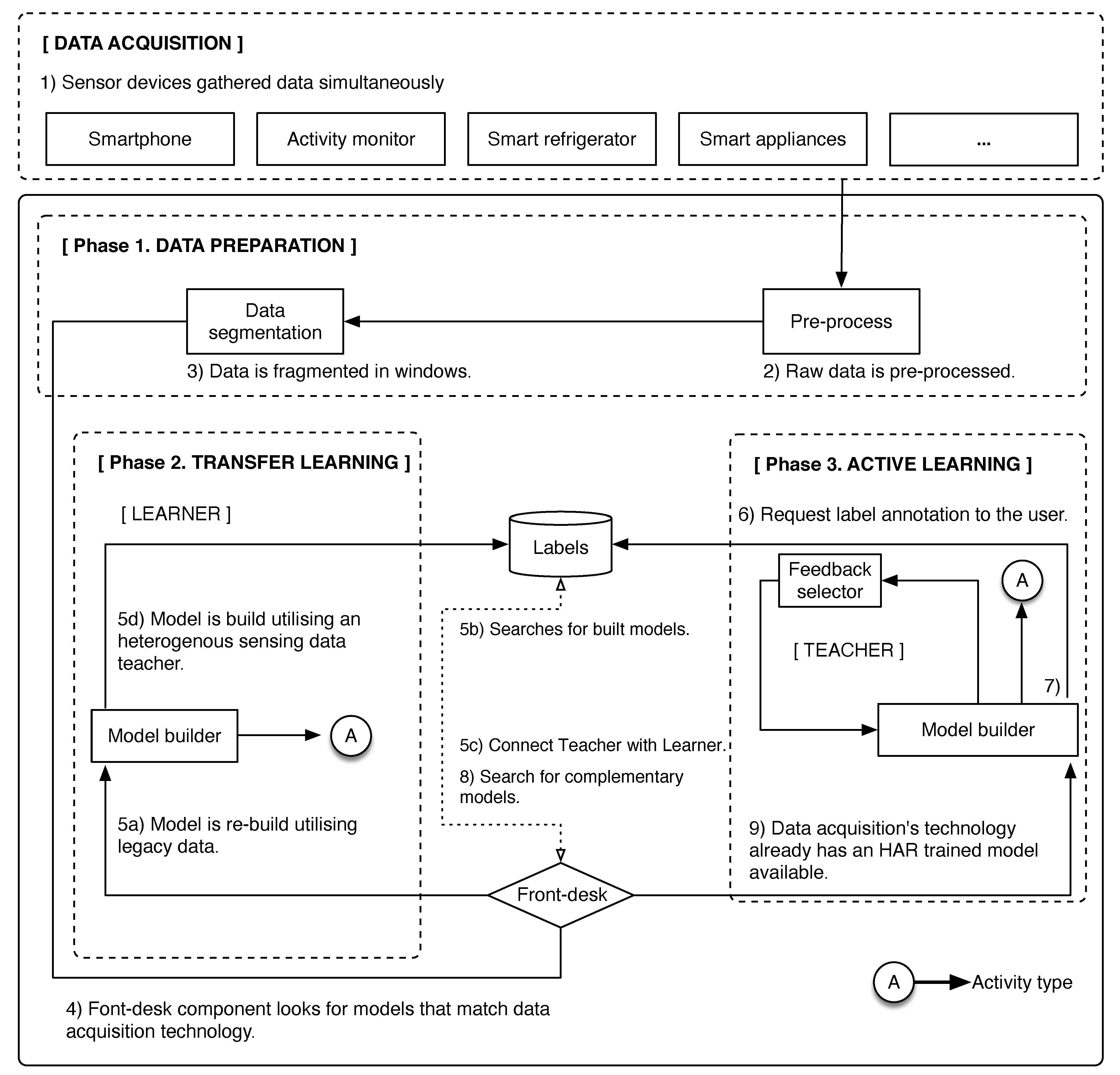
Algorithm 10 Organised list of the TL-FmRADL’s algorithms in order of execution as introduced in Figure 1.

INPUT: Step 1. Sensor devices gather data simultaneously. OUTPUT: Activity type   Phase 1. Data preparation Step 2. Raw data are pre-processed. Step 3. Data are fragmented in windows.   Phase 2. Transfer Learning Step 4. Front-desk component looks for modules that match data acquisition  technology. —Algorithm 1, Algorithm 2, Algorithm 3 Step 5. Model is re-build utilising legacy data. —Algorithm 4, Algorithm 5   Phase 3. Active Learning Step 6. Request label annotation to the user. —Algorithm 6 Step 7. Model is build. —Algorithm 7 Step 8. Search for complementary models. —Algorithm 7, Algorithm 8 Step 9. Data acquisition’s technology already has an HAR trained model  available. —Algorithm 7, Algorithm 9

4. Experiment Setup

To validate TL-FmRADLs this Section presents the development of two different experiments where its main components, namely, T/L and AL, are separately so that one can better appreciate how the learner model improved throughout TL-FmRADLs’ stages.

4.1. Teacher/Learner

The first experiment investigated the extent to which a teacher AR mode contributed to a learner model. It used a dataset segmented in four semi-labelled subsets per subject, where each subset corresponded to a variation relating to the amount of labelled data to be transferred from the teacher to the learner models (

Table 1. Semi-labelled subset for validating the T/L technique, where the ratio value represents the amount of data shared by the teacher to the learner model, where the ratios of data were randomly allocated.

Alternative	Ratio of Labelled Data Shared by the Teacher Model: Unshared Data
T/L100	100:0
T/L075	75:25
T/L050	50:50
T/L025	25:75

). Such design criteria would then allow measuring the impact on the classification performance achieved by the teacher model relative to the amount of labelled data available, where if the T/L concept were feasible, one would expect an improvement of the AR model as more teaching is provided.

The first experiment building on the evaluation of the T/L approach consisted of adopting one domain of technology as a teacher while the rest adopted the role of a learner. In particular, the thermal image model was selected as a teacher, whereas the inertial and audio models became the learners.

4.2. Active Learning

The second experiment was built on the evaluation for the AL approach and consisted of progressively queuing an oracle (Learner model) to retrieve its sensing features. This phase investigated the extent to which the feature fusion contributes to improving the performance of learner models under the schema of AL. It is important to highlight that this experiment built upon the previous learner model trained over the T/L phase. To evaluate this experiment, four sub-datasets were created, concatenating data as a new feature, as presented in

Table 2. Sub-datasets where features from a complementary sensing domain are included as part of the AL technique, where the ratios of data were randomly allocated.

Alternative	Ratio of Data to Concatenated: Data Missing Concatenation
AL100	100:0
AL075	75:25
AL050	50:50
AL025	25:75

.

5. InSync Dataset

The evaluation used the InSync dataset, a dataset collected at the pervasive computing lab at Ulster University, introduced for the first time upon this paper. It consists of subjects performing ADLs in a simulated home environment while data are collected by three different sensing technologies, namely, inertial, image, and audio.

InSync contains 12 h of data from ten subjects, consisting of 78 runs (times that a subject performed the scripted protocol). Sensor data from three different technologies (inertial, images, and audio) captured the performance of the subjects. All the activities were annotated a posteriori using a video stream.

The data collection study was carefully designed to provide realistic data. To this end, the study was conducted in an atmosphere that mimics a real-life environment. Additionally, although the subjects were given a set of ADLs, they were encouraged to perform the activities in a naturalistic way.

5.1. Activities of Daily Living

Considering that ADLs can be broken down into five categories: (i) Personal hygiene, such as bathing, grooming, oral and hair care; (ii) Continence, as a person’s ability to make use of the bathroom/toilet; (iii) Dressing, as a person’s ability to put on clothes; (iv) Feeding themselves; and (v) Transferring, the ability to walk independently [40]. InSync was built from four out of these five categories. It excluded the categories of continence given the privacy invasion that it will require to monitor it. The specific activities were:

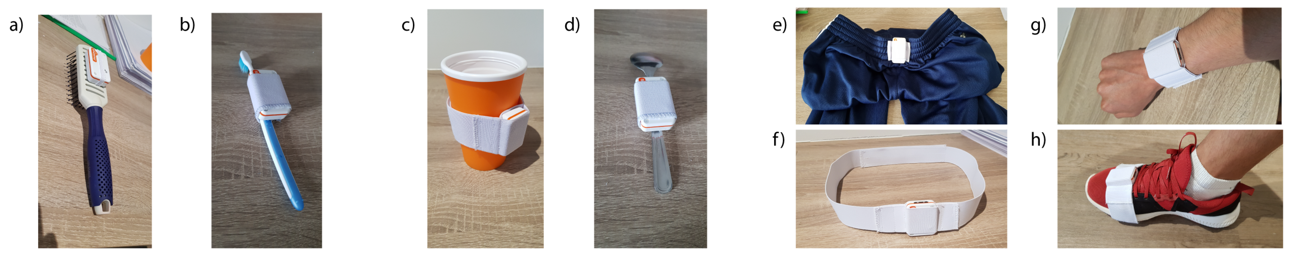
• Personal hygiene: comb hair, brush teeth;
• Dressing: put joggers on and off;
• Feeding: drink water from a mug and use a spoon to eat cereal from a bowl;
• Transferring: walk.

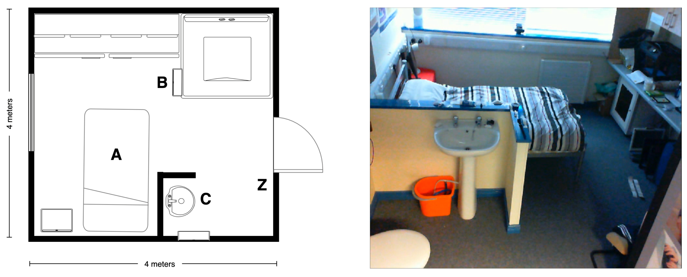
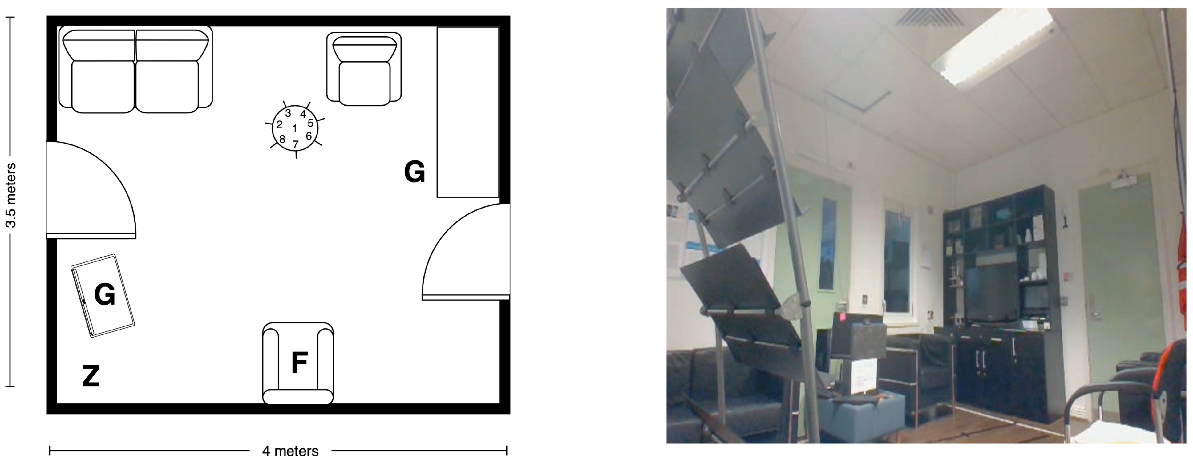
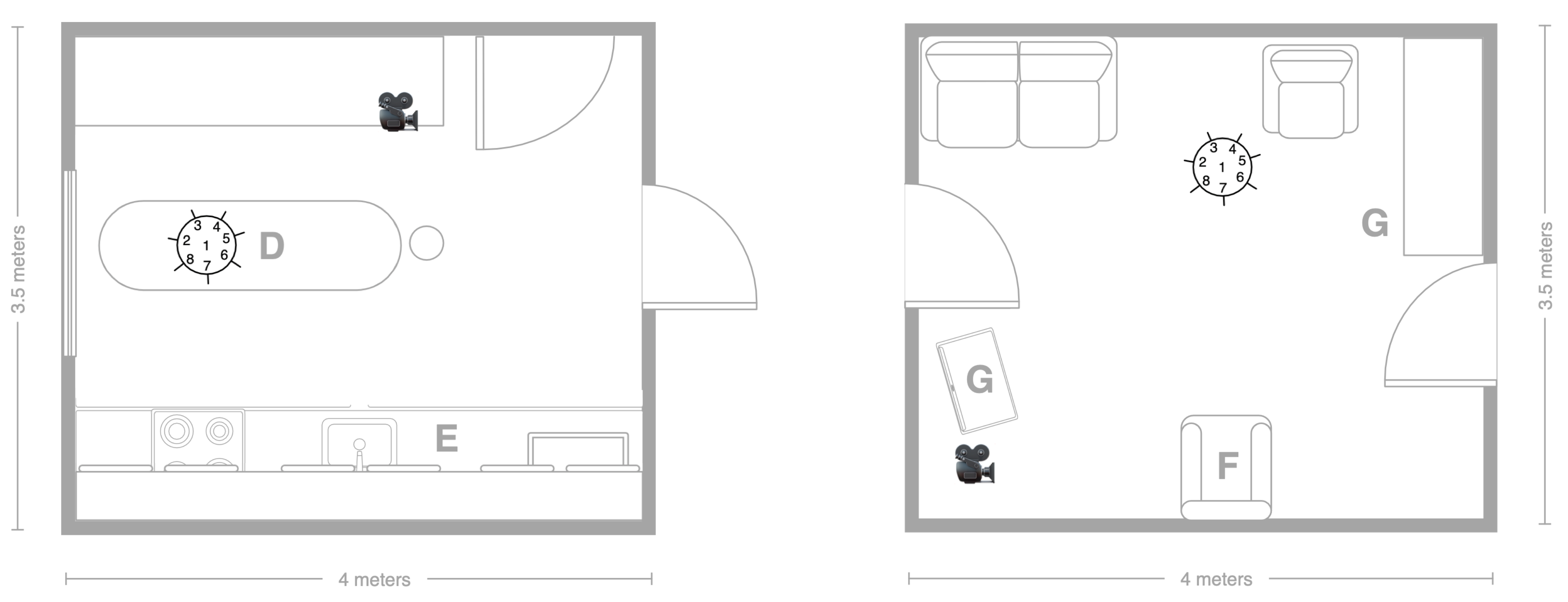
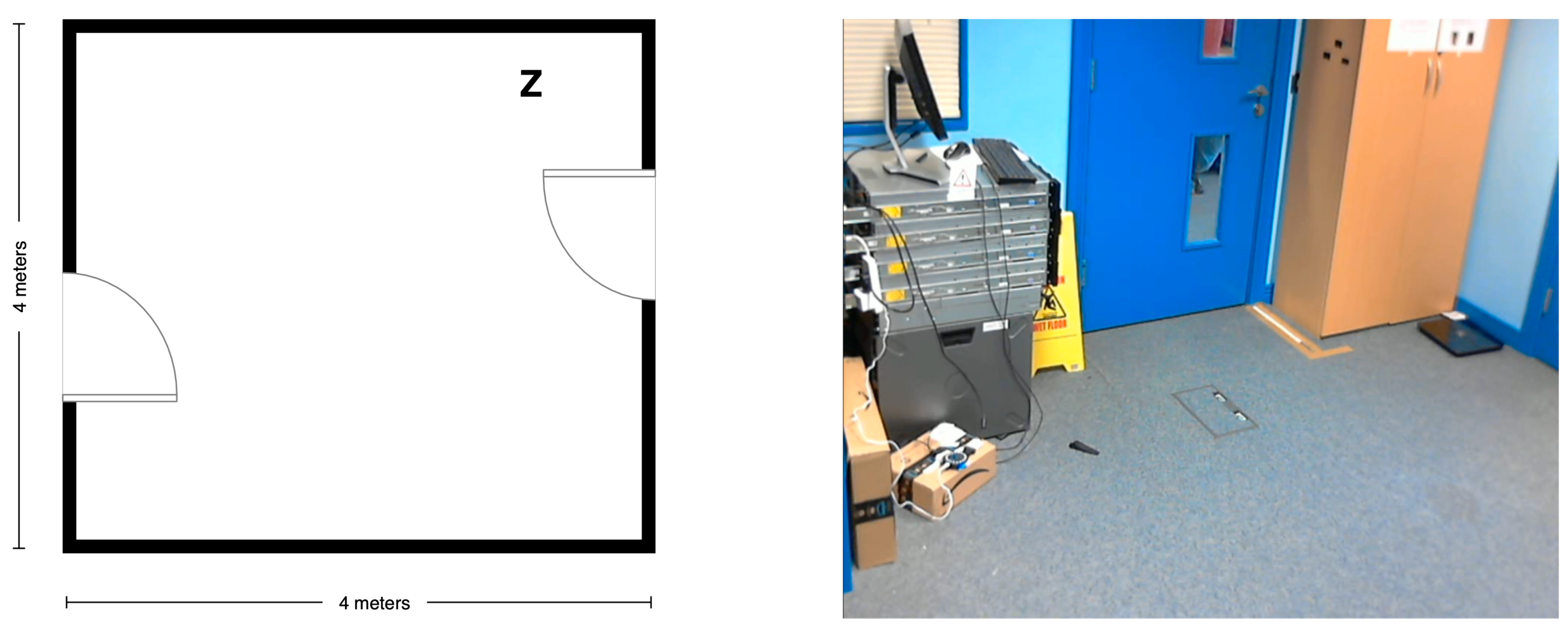
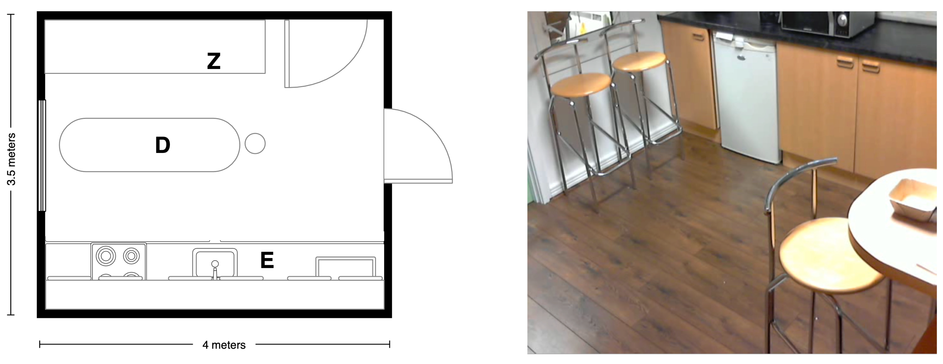
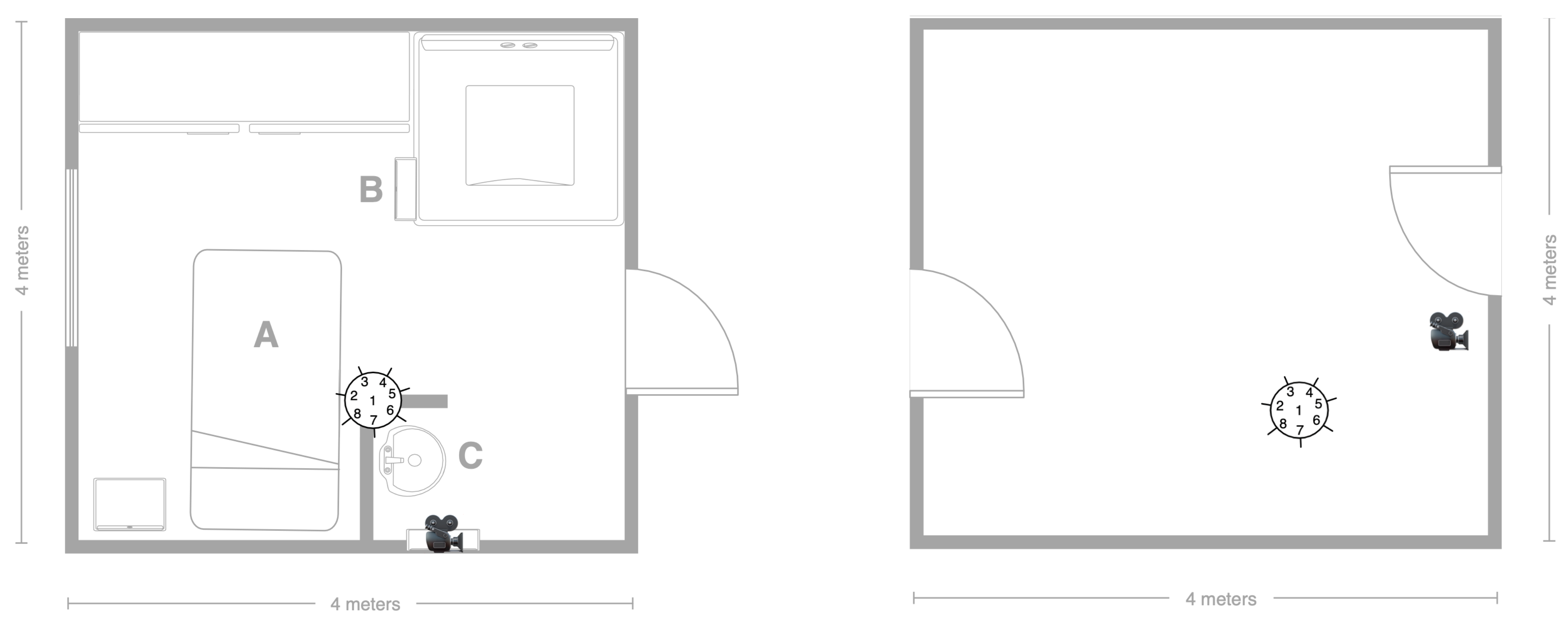
5.2. Recording Scenario

InSync was collected within the facilities of the smart environment from the pervasive computing labs at Ulster University, which mimics a daily life bedroom, bathroom, kitchen, and living room setting.

The bedroom consisted of a 4 × 4 m space fitted with an single size bed (A), a small stool (B), a toilet and large mirror (C) and a shower area at the right-up corner (not utilised in this study), as depicted in Figure 2. The adjacent room shown in Figure 3, consisted of a space free of obstacles which were considered as part of this study, so data from subjects interacting with the doors and walking could be recorded.

As depicted in Figure 4, the kitchen consisted on a 4 × 3.5 m space fitted with a (D) dinner table which includes a stool, (E) cabinets/cupboard, among other elements not utilised in this study, such as an electric stove, one sink, one small microwave, and a mini-fridge. The adjacent room consisted of a living room that included a free of obstacle area with a (F) chair and two (G) bookshelves as depicted in Figure 5.

5.3. Scripted Protocol

The dataset aimed at recording the subject’s physical activity performance. The tasks consisted of ADLs and well-known scenarios. Three general scenarios were chosen, a bedroom-related scenario in which the subjects performed two of the ADLs, namely, personal hygiene and dressing [41,42,43], a breakfast-related scenario was chosen to embrace the ADL of feeding as it has extensively been used in literature [44,45,46], and free of obstacle scenario in which the subjects can walk alongside to demonstrate their transferring capabilities [44,46]. The script was designed with nine high-level activities (napping, wearing joggers, brushing teeth, combing hair, operating door, eating cereal, drinking, walking, and standing) to which the subjects were encouraged to perform as naturally as possible (Note that the activities were performed not simulated).

5.4. Technology

The dataset is collected from three different technologies: Wearable computing consisting of sensors worn by the subjects, Smart-items consisting of sensors mounted on kitchen appliances and grooming items, and environmental sensors consisting of microphones, and thermal and binary sensors.

Overall, the deployed sensing technology included ten shimmer devices [47] enabled with 3-axis accelerometers, four matrix voice ESP32 [48] consisting of eight embedded microphones, four thermal vision sensors (TVSs) [49] and ten binary sensors, where the binary sensors were exclusively used to support with the synchronisation of the sensing data.

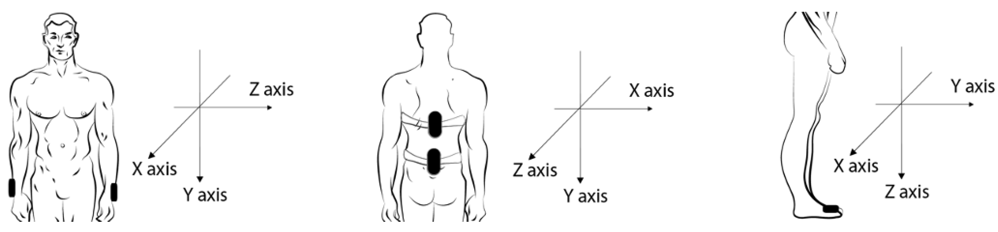
5.4.1. Wearable Domain

This technological domain consisted of five shimmer sensors enabled with 3-axis accelerometers working at a sample rate of 1.344 kHz (It should be noticed that the sample rate consists of high speed intending to create a robust dataset, so further researchers can experiment with it by down-sampling as needed). This device simulates the use of daily life smart gadgets and garments, such as smartwatches [50], clothing [51], and shoes [52]. To capture a broader set of movements as possible, the subject’s wore one sensor on each wrist, one at the lower back, one at the upper back and one on the right shoe, as depicted in Figure 6.

Worn sensors were placed where gadgets are commonly located, such as smartwatches (Figure 7g) worn on the wrist, smart shoes (Figure 7h) mounted on feet and garments (Figure 7f), such as belts along the hips.

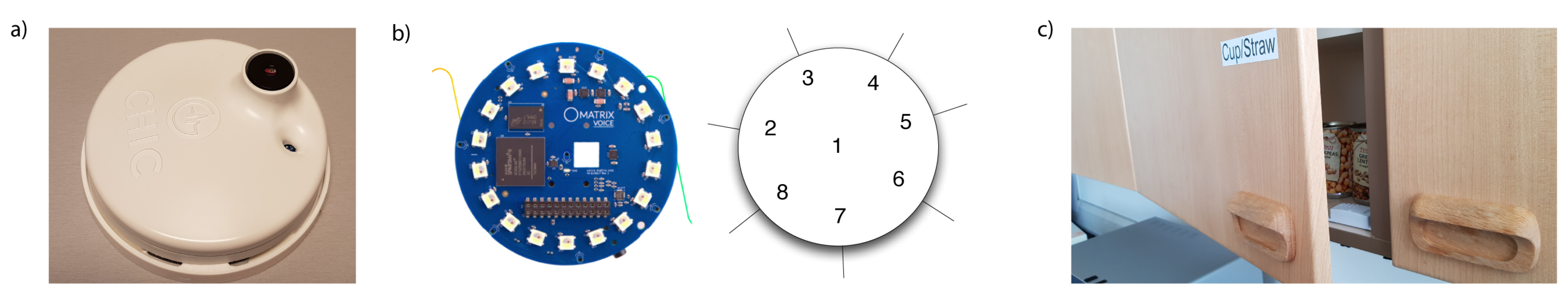
5.4.2. Smart-Items Domain

To capture the subject’s performance while executing ADLs, the dataset utilised five shimmer sensors mounted on everyday items, such as a hairbrush and toothbrush for grooming (Figure 7a,b), a cup and spoon for feeding (Figure 7c,d), and joggers to be worn along the hips (Figure 7e). Each smart-item has a binary sensor attached to keep track of the time when they were picked by the subjects.

5.4.3. Environmental Domain

This technological domain consisted of four TVS and four matrix voice ESP32 devices allocated in places nearby where the activities were being performed from each of the laboratory’s rooms as shown in Figure 8 and Figure 9. The TVS were strategical positioned in a way to capture the subject movements when performing the ADLs, such as the bathroom mirror where the subject would comb their hair, close to doors to capture the arm action of opening, and next to the dinner table where the subject would eat cereal and at a position where one could appreciate the subject transporting.

The TVS (Figure 10a) were enabled with real-time processing, which captured its frames using from the thermal lenses installed at strategical places in the different smart-rooms of the lab. The vision-based image processing captured every single thermal frame obtained from the TVS and applies a binary threshold which lowers the noise within the threshold. The matrix voice ESP32 were enabled with the eight embedded microphones to capture the acoustic yielded from the subject performing ADL (Figure 10b).

Binary sensors were mounted on each of the rooms’ door and kitchen cupboard (Figure 10c) to keep track of the time when they were being operated by the subjects.

5.5. Annotations

To facilitate the activity annotation, video recording was taken for the duration of data collection. The annotations consisted of nine high-level activities, namely, napping, wearing joggers, brushing teeth, combing hair, operating door, eating cereal, drinking, walking, and standing.

5.6. Subjects

Data were collected with the voluntary support of ten faculty-student and staff members from the School of Computing at Ulster University. The age range was of 25 to 33 years old ($\overline{x}$: 26.1, $\sigma$: 5.7 years). Subjects self-certified their health and signed an ethical consent letter beforehand. Data collection granted according to ethical governance from Ulster University.

5.7. Data Collection and Preparation

Subjects were instructed to perform as many repetitions or runs of the scripted protocol (Section 5.3) as possible. Overall, 62 runs were performed by the subjects; however, due to logistic difficulties (One TVS was not turned one due to neglect of the researcher), and technical complications consisting of malfunctions (One computer automatically turned off a couple of times when the processor overheated, one matrix voice ESP32 froze once unexpectedly) in the computers utilised to support with the capture of data and lost of connectivity to sensors (No data were captured from a thermal sensor as the Ethernet cable unplugged), five runs were excluded, as detailed in

Table 3. Relationship for the runs performed by each subject.

Subject	Performed Runs	Excluded Runs	Total
S01	8	2	6
S02	8	0	8
S03	4	0	4
S04	7	0	7
S05	6	1	5
S06	5	0	5
S07	6	0	6
S08	6	1	5
S09	6	0	6
S10	6	1	5
Total	62	5	57

.

Overall, it was identified that 0.5% of the raw inertial data was missing due to connectivity issues. Hence, to compensate such missed data, new data were imputed based on the mean value corresponding to the last second (i.e., 1344 data points) of the inertial data [53].

To mimic the sensing capabilities of commercial smart-items [54,55], the inertial data were down-sampled to 100 Hz [56]. To keep consistency of the time across the different sensing technology, all data were synchronised accordingly to the clock from the binary sensors (as it was observed to be more stable compared to the other sensors’ technology). Data segmentation was then performed by first defining time t as a starting point (t = 0) over the synchronised data. Then data were segmented into windows of two seconds with a step of one-second as proven effective by different researchers [57,58]. The dataset was pre-processed using Matlab 2018b.

6. Machine-Learning Modelling

Two critical characteristics of TL-FmADLs are the capability to transfer knowledge across sensing technology, and the improvement of AR models derived from AL techniques. To this extent, we built three AR models, each trained under one sensing technology, i.e., AR inertial model, AR images model, and AR audio model.

Note that, for the three models, cross-entropy loss function was used to measure the error between the prediction and the true values. Adam [59], which is a stochastic optimisation algorithm, was selected as the optimiser, as it has shown to be effective in resolving classification problems [60,61,62,63].

(i) AR Inertial model.

Consisting of the sensing devices worn by the subject and embedded into smart-items, the feature-space embodies the root mean square (RMS) and the mean of each of the three axes from both acceleration and gyroscope data.

This machine-learning model conceived a one-dimensional DNN with a learning rate of 0.001. Its first layer received a tensor of six features per smart-item; hence 60 features in total. It then structured three hidden layers assembled over the rectified linear unit (ReLU) and an output layer consisting of the softmax activation function (as it proved effective in the results in training DNN models [21,64,65]).

(ii) AR Images model.

Consisting of the images captured by the TVS device, the feature-space embodies the thermal images in grey-scale rather than RGB images to reduce the computational cost [66], where features were extracted over a fully connected CNN for 32 × 32 pixel images.

This machine-learning model conceived a three-dimensional CNN with a learning rate of 0.0001. Its first layer received a tensor of 32 × 32 × 3 (width, height, depth). It then structured three hidden layers, assembled over max-pool and normalised convolutional layer, followed by three layers under ReLU activation function.

(iii) AR Audio model.

Consisting of the acoustic data captured by the matrix voice ESP32, the feature-space embodies eight elements: energy entropy, short-time energy, spectral roll-off, spectral centroid, spectral flux, zero-crossing rate, relative spectral transform, and Mel-frequency spectral coefficients.

This machine-learning model conceived a one-dimensional DNN with a learning rate of 0.001. Its first layer received a tensor of eight features. It then structured three hidden layers, assembled over the ReLU, and an output layer consisting of the softmax activation function. The DNN models were created utilising machine-learning libraries such as TensorFlow and Keras.

It is important to highlight that AR systems are typically evaluated for their ability to generalise their AR models’ capabilities after being trained. In this regard, a commonly investigated problem is the representation of AR models to generalise across subjects, which bring different challenges derived from the dependency on subjects’ performance, i.e., population-based versus personal-based training [67]. Hence, in the interest of investigating the transfer learning capabilities across sensor, the AR models focused on personal-based training by evaluating the impact of TL-FmADLs per subject.

The performance was evaluated under 10-fold cross-validation [68]. The initiation weight was randomly allocated and mini-batches with shuffling adopted as a strategy to counterbalance the problem of non-convexity [68].

7. Results

Due to the random initiation of the DNN, the classification models were susceptible to fall within the problem of non-convexity; where the models could fall within the local minimum. To counteract this phenomenon, the AR models iterated ten times.

7.1. Baseline

To evaluate the contribution of the T/L and AL techniques, results were compared against a baseline acquired by evaluating the performance of the three AR models, namely, AR inertial model, AR image model, and AR audio model.

Table 4. Average classification accuracy (expressed in percentage) for the inertial model trained to classify the performance of the AR models of the ten subjects that participated within the data collections of InSync dataset.

Subject	Average	Standard Deviation
S01	95.2	0.8
S02	96.2	2.0
S03	91.7	3.4
S04	90.2	2.2
S05	88.8	2.9
S06	92.9	1.5
S07	89.9	1.9
S08	90.6	1.2
S09	86.8	2.0
S10	87.5	2.1

presents the results for the baseline classification accuracy of the Inertial model. The average performance for the classification accuracy was 91.0% with a minimum accuracy of 86.8% for S09 and maximum accuracy of 96.2% for S02.

Table 5. Average classification accuracy (expressed in percentage) for the audio model trained to classify the performance of the AR models of the ten subjects that participated within the data collections of InSync dataset.

Subject	Average	Standard Deviation
S01	78.9	0.6
S02	76.7	2.5
S03	62.7	0.7
S04	57.0	7.4
S05	71.3	0.4
S06	70.1	0.6
S07	62.8	5.6
S08	67.2	0.4
S09	69.0	4.0
S10	69.0	0.5

presents the results for the baseline classification accuracy of the audio model. The average performance for the classification accuracy was 68.5% with a minimum accuracy of 57.0% for S04 and maximum accuracy of 78.9% for S01.

Table 6. Average classification accuracy (expressed in percentage) for the image model trained to classify the performance of the AR models of the ten subjects that participated within the data collections of the InSync dataset.

Subject	Average	Standard Deviation
S01	99.0	0.9
S02	98.9	0.4
S03	99.0	0.6
S04	95.4	0.7
S05	92.5	0.6
S06	97.9	0.5
S07	94.4	1.0
S08	93.5	0.8
S09	91.4	0.5
S10	90.9	1.1

presents the results for the baseline classification accuracy of the Images model. The average performance for the classification accuracy was 95.3% with a minimum accuracy of 90.9% for S09 and maximum accuracy of 99.0% for S01 and S03.

7.2. Teacher/Learner

As introduced early, to evaluate the performance of the T/L approach a teacher and a learner model were defined. Derived from the baseline performance achieved by the AR Image model which reached an average classification accuracy of 95.3%; representing a difference of 4.3% and 26.8% compared to the inertial-learner model and audio-learner, respectively. The AR image model was defined as the teacher model underlined in this evaluation.

Hence, to evaluate the performance of the Learner models, two experiments were undertaken. Firstly, one experiment where the AR inertial model played the role as a learner, followed by the second experiment, in which the AR audio model played the role as learner.

Results from the first experiment consisting of training the inertial-learner model over the teacher’s are presented in

Table 7. Relationship to compare the performance of the inertial-learner average classification (expressed in percentage) model trained over the T/L approach in contrast to the baseline.

Subjects	Inertial-Learner Baseline	T/L100	T/L075	T/L050	T/L025
S01	95.2	95.9	95.9	95.4	95.5
S02	96.2	99.1	99.0	99.0	99.0
S03	91.7	93.2	93.2	93.1	92.9
S04	90.2	91.4	92.2	92.2	92.3
S05	88.8	84.6	91.6	89.4	86.1
S06	92.9	93.5	94.7	94.6	95.0
S07	89.9	88.7	92.8	92.8	92.3
S08	90.6	92.8	92.1	92.5	92.8
S09	86.8	89.0	91.7	91.8	91.5
S10	87.5	83.8	90.2	89.5	86.2
Average	91.0	91.2	93.4	93.0	92.3

. The table shows the outcome from four sub-datasets T/L100, T/L075, T/L050, and T/L025, which represents the amount of labelled data shared by the learner model (i.e., 100%, 75%, 50%, and 25%), as rationalised in Section 4.1.

The table contrasts the baseline against the performance from the T/L classification accuracy when the AR inertial model adopted the role as a learner. As it can be observed, the highest performance was reached when training under the alternative T/L075 (93.4%), with a difference of 2.5% compared to the baseline (91.0%).

Results from the second experiment consisting of training the audio-learner model over the teacher’s are presented in

Table 8. Relationship to compare the performance of the audio-learner average classification (expressed in percentage) model trained over the T/L approach in contrast to the baseline.

Subjects	Audio-Learner Baseline	T/L100	T/L075	T/L050	T/L025
S01	78.9	78.9	79.0	78.6	79.3
S02	76.7	77.0	77.8	77.6	77.7
S03	62.7	65.2	65.7	65.6	65.8
S04	57.0	68.5	68.9	68.7	68.6
S05	71.3	67.7	73.0	70.1	68.3
S06	70.1	70.8	71.8	70.7	70.7
S07	62.8	71.3	73.3	72.8	72.0
S08	67.2	68.0	68.9	67.8	68.0
S09	69.0	71.0	72.9	73.0	72.3
S10	69.0	65.3	70.9	70.1	68.3
Average	68.5	70.4	72.2	71.5	71.1

. As it can be observed, in this experiment the highest performance was reached when training under the alternative T/L075 (72.4%), with a difference of 3.7% compared to the baseline (68.5%).

7.3. Active Learning

As introduced earlier, to evaluate the performance of the AL approach. Derived from the baseline performance achieved by the AR Image model which reached an average classification accuracy of 95.3%; representing a difference of 4.3% and 26.8% compared to the inertial-learner model and audio-learner model, respectively. The AR image model was defined as the teacher model underlined in this evaluation.

Hence, to evaluate the performance of the Learner models, two experiments were undertaken. Firstly, one experiment where the AR inertial model played the role as a learner, followed by the second experiment, in which the AR audio model played the role as learner.

The evaluation consisted of progressively queuing the learner model to retrieve its sensing features to fuse with the learner model. To illustrate the benefit of this mechanism, the study defined four sub-dataset of data split into segments of 25% each. In this context, the baseline results were compared against the performance of the classification model when utilising 100%, 75%, 50%, and 25% of labelled data retrieved from the oracle, as rationalised in Section 4.2.

Results from the AL approach are shown in

Table 9. Relationship to compare the performance of the Inertial average classification (expressed in percentage) model in contrast to the baseline and the four different alternatives over the AL approach.

Subjects	Inertial-Learner Baseline	AL100	AL075	AL050	AL025
S01	95.2	97.2	97.0	93.1	91.0
S02	96.2	97.0	98.6	98.5	96.3
S03	91.7	97.2	93.4	92.8	91.6
S04	90.2	98.6	96.7	94.3	91.1
S05	88.8	96.6	92.6	89.3	88.6
S06	92.9	98.4	97.0	95.0	93.7
S07	89.9	93.2	92.6	91.7	90.8
S08	90.6	92.0	91.5	90.1	88.8
S09	86.8	96.1	95.6	89.3	86.7
S10	87.5	94.4	94.8	90.8	88.9
Average	91.0	96.1	95.0	92.5	90.8

. The table contrasts the baseline against the performance from the AL classification accuracy when the inertial model adopts the role as a learner model and it is trained under the schema of AL. The overall difference as presented under the row ‘Average’, shows the best performance when 100% of the learner model labels are used, consisting of 96.1%.

Similarly,

Table 10. Relationship to compare the performance of the audio average classification (expressed in percentage) model in contrast to the baseline and the four different alternatives over the AL approach.

Subjects	Audio-Learner Baseline	AL100	AL075	AL050	AL025
S01	78.9	95.2	87.6	80.7	74.3
S02	76.7	93.5	88.1	79.2	75.5
S03	62.7	94.6	86.1	77.7	72.0
S04	57.0	96.5	86.8	79.5	73.7
S05	71.3	95.5	87.1	80.5	73.8
S06	70.1	96.4	89.2	81.2	73.5
S07	62.8	93.4	86.1	78.8	75.5
S08	67.2	89.2	84.2	77.8	70.7
S09	69.0	93.0	87.4	79.8	73.2
S10	69.0	93.1	87.9	79.9	71.5
Average	68.5	94.0	87.0	79.5	73.4

contrasts the baseline against the performance from the AL classification accuracy when the audio model adopts the role as a learner and gradually queried the oracle. The average difference is presented in the row ‘Average’, which shows the best performance when the learner model queried 100% of the labels provided by the learner model, consisting of 94%.

The following tables compare the baselines from both learner models (inertial-learner and audio-learner), teacher model (image-teacher) against the performance achieved by the learner models when completing the proposed method training (column ‘Fusion stage’). Specifically,

Table 11. Comparison of the average classification accuracy (expressed in percentage) of the performance achieved when the Inertial-Learner model is trained over TL-FmRADLs against the baseline performance of the image-teacher model.

Subjects	Inertial-Learner	Image-Teacher	Inertial-Learner (Fusion Stage)
S01	95.2	99.0	97.2
S02	96.2	98.9	97.0
S03	91.7	99.0	97.2
S04	90.2	95.4	98.6
S05	88.8	92.5	96.6
S06	92.9	97.9	98.4
S07	89.9	94.4	93.2
S08	90.6	93.5	92.0
S09	86.8	91.4	96.1
S10	87.5	90.9	94.4
Average	91.0	95.3	96.1

shows the performance when the inertial-learner model completed the TL-FmRADLs process, and

Table 12. Comparison of the average classification accuracy (expressed in percentage) of the performance achieved when the audio-learner model is trained over TL-FmRADLs against the baseline performance of the image-teacher model.

Subjects	Audio-Learner	Image-Teacher	Audio-Learner (Fusion Stage)
S01	78.9	99.0	95.2
S02	76.7	98.9	93.5
S03	62.7	99.0	94.6
S04	57.0	95.4	96.5
S05	71.3	92.5	95.5
S06	70.1	97.9	96.4
S07	62.8	94.4	93.4
S08	67.2	93.5	89.2
S09	69.0	91.4	93.0
S10	69.0	90.9	93.1
Average	68.5	95.3	94.0

shows the performance when the audio-learner model completed the TL-FmRADLs process.

Results of this study showed the benefit of utilising TL-FmRADLs, which relies upon feature fusion and T/L techniques to increase the performance of the classification accuracy underlined by an AL to enable an automatic approach.

7.4. Comparison

To allow a better comparison of TL-FmRADLs performance against state-of-the-art research in AR, this Section compares four different studies presenting different approaches to transfer knowledge across sensors.

• Radu and Henne [69] presented a method to transfer knowledge where the teacher consisted of mainstream sensing (video) to provide labelled data to the inertial sensors embracing the role as learners;
• Rey et al. [70] proposed a method that works by extracting 2D poses from video frames and then used a regression model to map them to inertial sensors signal;
• Hu and Yang [22] presented a paper in which they used Web knowledge as a bridge to help link the different label spaces between two smart environments. Their method consisted of an unsupervised approach where features were clustered based in their distribution; hence, even though the feature’s space were different, their distribution distance helped to build an association to transfer knowledge.
• Xing et al. [71] presented two methods (PureTransfer and Transfer+LimitedTrain) for transferring knowledge. For the purposes of this state-of-the-art comparison, only the method reporting highest performance was taken into account (i.e., Transfer+LimitedTrain). Transfer+LimitedTrain method consisted of a DNN which added higher layers to the new targeted model, where only the higher layer is retrained.

Notice that, since the algorithms described in the aforementioned research have different settings compared to those adopted in this evaluation, we cannot use their algorithms to compare their performance when training over InSync. Hence, the comparison should be made based upon the improvement (i.e., baseline ≠ accuracy achieved).

The different studies mentioned above are enlisted in

Table 13. Comparison of TL-FmRADLs’ performance against state-of-the-art approaches, where CPP stands for contact movement, passive infrared, pressure, and CIA stands for contact movement, image, audio.

Research Method	Teacher	Learner	Baseline	Achieved	Improvement
Radu and Henne [69]	Image	Inertial	95.4	97.1	1.7
Rey et al. [70]	Image	Inertial	85.0	90.0	5.0
Hu and Yang [22]	CPP	CIA	47.3	59.8	12.5
Hu and Yang [22]	CIA	CPP	42.8	61.2	18.4
Xing et al. [71]	Inertial	Image	72.3	75.1	2.9
Xing et al. [71]	Inertial	Audio	84.3	87.8	3.5
Xing et al. [71]	Image	Audio	84.1	90.4	6.2
Xing et al. [71]	Image	Inertial	70.7	94.4	23.6
TL-FmRADLs	Image	Inertial	91.0	96.1	5.1
TL-FmRADLs	Image	Audio	68.5	94.0	25.5

, where different sensing technology has been used. The ‘Baseline’ column represents the accuracy performance achieved by the machine-learning models before implementing the transfer learning approach proposed within the different researches. The performance achieved is presented under the column ‘Achieved’, where the comparison difference is presented under the column ‘Improvement’.

Results of this comparison show TL-FmRADLs outperforming the other approaches with reporting a 25.5% improvement when transferring knowledge between image and audio sensors. It should be noticed that while transferring knowledge from image to inertial sensors only reached 5.1%, its classification performance is one of the highest compared to the other method’s rising to 96.1%; just followed by Radu and Henne’s method.

8. Discussion

This paper presented and evaluated TL-FmRADLs; a transfer learning framework for recognising activities of daily living across sensing technology. Three different AR models were designed defined by its sensing data as the AR image model, AR inertial model and AR audio model. Derived from the baseline experiment conducted, the AR image model was empirically determined as the teacher model, whereas the AR inertial and AR audio models adopted the role as learner.

Two experiments were presented, one showcasing the benefit of each of the main components implemented in TL-FmRADLs. Regarding the T/L phase, results showed that the highest average improvement in accuracy of 93.4% and 72.2% when training the inertial-learner model and the audio-learner model, respectively. It was observed that there was a fluctuation on the accuracy achieved when increasing the amount of training data from the alternative T/L075 to T/L100 (as shown in Table 7 and Table 8). Results suggested that transferring 100% of knowledge from the image-teacher model to the learners models (inertial and audio) trained the DNN models’ process to the extent of overfitting the model. In this regard, the performance diminished the classification accuracy of the objective AR subject’s model. Nevertheless, this finding can represent a positive finding, since one can assume that the performance of the AR model benefited from this method over a small portion of fusion labelled data, thereby implying a reduced computational cost.

As for the second experiment, the AL technique contributed by fusing features from a complementary sensing technology. Results showed the highest classification accuracy when converging the Image-teacher model and inertial-learner model, which reached 96.1%, representing an increase of 2.7% compared to the achievement under the T/L phase (93.4%). However, the highest gain was reflected when converging the image-teacher model and audio-learner model as shown by its classification accuracy, which increased from 72.2% (achieved at the T/L phase) to 94% (achieved at the AL phase), thereby reflecting an improvement of 21.8%. In general, one can rationalise that the learner model benefits from the teacher’s knowledge over converging T/L and AL techniques since the Learner models showed important improvements in both the experiment.

Finally, TL-FmRADLs was compared against five different methods reported in the literature. Such a comparison showed a more significant improvement for the learner model when transferring knowledge from an image-based model to an audio-based model with an improvement rising to 25.5%. It also showed improvement in models that had already achieved high performance in their baseline. In particular, the first experiment showed that when transferring knowledge from an image-based sensor to an inertial-sensor, the performance increased from 91% to 96.1% (an improvement of 5.1%), which, when compared to the other methods, was one of the highest performances achieved just after Radu and Henne.

9. Challenges and Research Directions

As presented in this paper, transfer learning, if carried out successfully, can significantly improve the performance of AR data-driven modelling. In this Section, we summarise and discuss the challenges faced and the potential research opportunities and future directions of this investigation.

TL-FmADLs was introduced as a transfer learning framework to automate machine-learning modelling. Although TL-FmADL was evaluated utilising InSync, one should note that the data collection was conducted in a simulated home environment over a scripted set of ADLs. To this end, TL-FmADL can develop further through an evaluation using data collected under natural conditions and an extended number of subjects, where subjects would perform their ADLs without guidelines, and the larger number of subjects could allow us to generalise the results better. This activity can address two issues. First, it could evaluate the classification capabilities of unpredicted human behaviour. Second, it could assess the latency and response time for the computation component, which could impact the performance of the modelling process.

Moreover, one can observe that the $FrontDesk$ component seeks compatible machine-learning models to refer to as teachers. Although current experimentation was conducted utilising annotations to categorise each machine-learning model, a more robust approach can be planned. In particular, one can envision the formatting style proposed for the open data initiative (ODI) to represent data obtained from sensors [72]. ODI is an ontological model that includes a common protocol for data collection, a common format for data exchange, a data repository, and related tools to underpin research within the domain of activity recognition. ODI utilises the extensible event stream (XES) standard for event data storage [73] and an ontological model for the description of experimental metadata, which has been designed to address issues surrounding the management, storage, and exchange of sensing data [74]. In this regard, one can anticipate the availability of contextual information to characterise the environment in which the ADL is taking place, to optimise the framework’s searching processes.

10. Concluding Remarks

This paper’s contribution comprised two elements. First, it detailed the evaluation of TL-FmRADLs: a transfer learning framework for recognising activities of daily living across sensing technology. Second, it introduces InSync: a dataset comprising sensing data from three different sensing technologies, namely, audio, thermal images, and inertial data, as ten subjects performing ADLs in a scripted fashion under a simulated home environment.

TL-FmRADLs proposes a mechanism for mitigating the insufficiency of labelled data across sensing technologies by leveraging the performance of learner models using feature fusion as a strategy and enabling the automatisation for self-training over the AL technique. The evaluation comprised two experiments: one showcasing the benefit of the T/L phase and another focusing on the AL phase.

As for the first contribution, the TL-FmRADLs was compared against five other methods reported within the literature, where it showed promising results. The proposed framework exhibits promising applications in scenarios where adaptation is important due to the uncertainty of new data, as occurs in modelling problems for ADLs. The second contribution consisting of a dataset, namely InSync, will be available to the research community upon the publication of this paper as specified within the data availability statement presented next.

It is important to consider that the run-time classification complexity of combining the T/L and AL phases was not evaluated; however, considering the processor capability of modern mobile devices, it was hypothesised that the implementation is suitable for real-time recognition in mobile platforms. Nevertheless, due to the topic’s importance, it can be relevant to investigate real-time performance in realistic scenarios, which is a study that may be undertaken as part of further work.

References

1. Hernandez, N.; Lundström, J.; Favela, J.; McChesney, I.; Arnrich, B. Literature Review on Transfer Learning for Human Activity Recognition Using Mobile and Wearable Devices with Environmental Technology. SN Comput. Sci. 2020, 1, 1–16. [Google Scholar] [CrossRef] [Green Version]
2. Zhuang, F.; Qi, Z.; Duan, K.; Xi, D.; Zhu, Y.; Zhu, H.; Xiong, H.; He, Q. A Comprehensive Survey on Transfer Learning. Proc. IEEE 2020, 109, 43–76. [Google Scholar] [CrossRef]
3. Deep, S.; Zheng, X. Leveraging CNN and Transfer Learning for Vision-based Human Activity Recognition. In Proceedings of the 2019 29th International Telecommunication Networks and Applications Conference (ITNAC), Auckland, New Zealand, 27–29 November 2019; pp. 1–4. [Google Scholar]
4. Casserfelt, K.; Mihailescu, R. An investigation of transfer learning for deep architectures in group activity recognition. In Proceedings of the 2019 IEEE International Conference on Pervasive Computing and Communications Workshops (PerCom Workshops), Kyoto, Japan, 11–15 March 2019; pp. 58–64. [Google Scholar]
5. Alshalali, T.; Josyula, D. Fine-Tuning of Pre-Trained Deep Learning Models with Extreme Learning Machine. In Proceedings of the 2018 International Conference on Computational Science and Computational Intelligence (CSCI), Las Vegas, NV, USA, 12–14 December 2018; pp. 469–473. [Google Scholar]
6. Cook, D.; Feuz, K.D.; Krishnan, N.C. Transfer learning for activity recognition: A survey. Knowl. Inf. Syst. 2013, 36, 537–556. [Google Scholar] [CrossRef] [Green Version]
7. Hachiya, H.; Sugiyama, M.; Ueda, N. Importance-weighted least-squares probabilistic classifier for covariate shift adaptation with application to human activity recognition. Neurocomputing 2012, 80, 93–101. [Google Scholar] [CrossRef]
8. van Kasteren, T.; Englebienne, G.; Kröse, B. Recognizing Activities in Multiple Contexts using Transfer Learning. In Proceedings of the AAAI AI in Eldercare Symposium, Arlington, VA, USA, 7–9 November 2008. [Google Scholar]
9. Cao, L.; Liu, Z.; Huang, T.S. Cross-dataset action detection. In Proceedings of the IEEE Computer Society Conference on Computer Vision and Pattern Recognition, San Francisco, CA, USA, 13–18 June 2010. [Google Scholar]
10. Yang, Q.; Pan, S.J. A Survey on Transfer Learning. IEEE Trans. Knowl. Data Eng. 2010, 22, 1345–1359. [Google Scholar]
11. Hossain, H.M.S.; Khan, M.A.A.H.; Roy, N. DeActive: Scaling Activity Recognition with Active Deep Learning. Proc. ACM Interact. Mob. Wearable Ubiquitous Technol. 2018, 2, 1–23. [Google Scholar] [CrossRef] [Green Version]
12. Alam, M.A.U.; Roy, N. Unseen Activity Recognitions: A Hierarchical Active Transfer Learning Approach. In Proceedings of the 2017 IEEE 37th International Conference on Distributed Computing Systems (ICDCS), Atlanta, GA, USA, 5–8 June 2017; pp. 436–446. [Google Scholar]
13. Civitarese, G.; Bettini, C.; Sztyler, T.; Riboni, D.; Stuckenschmidt, H. NECTAR: Knowledge-based Collaborative Active Learning for Activity Recognition. In Proceedings of the 2018 IEEE International Conference on Pervasive Computing and Communications, Athens, Greece, 19–23 March 2018. [Google Scholar]
14. Civitarese, G.; Bettini, C. newNECTAR: Collaborative active learning for knowledge-based probabilistic activity recognition. Pervasive Mob. Comput. 2019, 56, 88–105. [Google Scholar] [CrossRef] [Green Version]
15. Wang, S.; Chang, X.; Li, X.; Sheng, Q.Z.; Chen, W. Multi-Task Support Vector Machines for Feature Selection with Shared Knowledge Discovery. Signal Process. 2016, 120, 746–753. [Google Scholar] [CrossRef]
16. Feuz, K.D.; Cook, D.J. Collegial activity learning between heterogeneous sensors. Knowl. Inf. Syst. 2017, 53, 337–364. [Google Scholar] [CrossRef] [PubMed]
17. Rokni, S.A.; Ghasemzadeh, H. Autonomous Training of Activity Recognition Algorithms in Mobile Sensors: A Transfer Learning Approach in Context-Invariant Views. IEEE Trans. Mob. Comput. 2018, 17, 1764–1777. [Google Scholar] [CrossRef]
18. Kurz, M.; Hölzl, G.; Ferscha, A.; Calatroni, A.; Roggen, D.; Tröster, G. Real-Time Transfer and Evaluation of Activity Recognition Capabilities in an Opportunistic System. In Proceedings of the Third International Conference on Adaptive and Self-Adaptive Systems and Applications, Rome, Italy, 25–30 September 2011. [Google Scholar]
19. Roggen, D.; Förster, K.; Calatroni, A.; Tröster, G. The adARC pattern analysis architecture for adaptive human activity recognition systems. J. Ambient. Intell. Humaniz. Comput. 2013, 4, 169–186. [Google Scholar] [CrossRef] [Green Version]
20. Calatroni, A.; Roggen, D.; Tröster, G. Automatic transfer of activity recognition capabilities between body-worn motion sensors: Training newcomers to recognize locomotion. In Proceedings of the Eighth International Conference on Networked Sensing Systems (INSS’11), Penghu, Taiwan, 12–15 June 2011. [Google Scholar]
21. Hernandez, N.; Razzaq, M.A.; Nugent, C.; McChesney, I.; Zhang, S. Transfer Learning and Data Fusion Approach to Recognize Activities of Daily Life. In Proceedings of the 12th EAI International Conference on Pervasive Computing Technologies for Healthcare, New York, NY, USA, 21–24 May 2018. [Google Scholar]
22. Hu, D.H.; Yang, Q. Transfer learning for activity recognition via sensor mapping. In Proceedings of the IJCAI International Joint Conference on Artificial Intelligence, Catalonia, Spain, 16–22 July 2011. [Google Scholar]
23. Zheng, V.W.; Hu, D.H.; Yang, Q. Cross-domain activity recognition. In Proceedings of the 11th International Conference on Ubiquitous Computing, Orlando, FL, USA, 30 September–3 October 2009; pp. 61–70. [Google Scholar]
24. Fallahzadeh, R.; Ghasemzadeh, H. Personalization without User Interruption: Boosting Activity Recognition in New Subjects Using Unlabeled Data. In Proceedings of the 2017 ACM/IEEE 8th International Conference on Cyber-Physical Systems (ICCPS), Hong Kong, China, 17–19 May 2017. [Google Scholar]
25. Settles, B. Active Learning Literature Survey; University of Wisconsin: Madison, WI, USA, 2010. [Google Scholar]
26. Wen, J.; Zhong, M.; Indulska, J. Creating general model for activity recognition with minimum labelled data. In Proceedings of the 2015 ACM International Symposium on Wearable Computers, Osaka, Japan, 9–11 September 2015. [Google Scholar]
27. Zhou, B.; Cheng, J.; Sundholm, M.; Reiss, A.; Huang, W.; Amft, O.; Lukowicz, P. Smart table surface: A novel approach to pervasive dining monitoring. In Proceedings of the 2015 IEEE International Conference on Pervasive Computing and Communications, St. Louis, MO, USA, 23–27 March 2015. [Google Scholar]
28. Hu, L.; Chen, Y.; Wang, S.; Wang, J.; Shen, J.; Jiang, X.; Shen, Z. Less Annotation on Personalized Activity Recognition Using Context Data. In Proceedings of the 13th IEEE International Conference on Ubiquitous Intelligence and Computing, Toulouse, France, 18–21 July 2017. [Google Scholar]
29. Saeedi, R.; Sasani, K.; Gebremedhin, A.H. Co-MEAL: Cost-Optimal Multi-Expert Active Learning Architecture for Mobile Health Monitoring. In Proceedings of the 8th ACM International Conference on Bioinformatics, Computational Biology and Health Informatics, Boston, MA, USA, 20–23 August 2017; ACM: New York, NY, USA, 2017; pp. 432–441. [Google Scholar]
30. Dao, M.S.; Nguyen-Gia, T.A.; Mai, V.C. Daily Human Activities Recognition Using Heterogeneous Sensors from Smartphones. Procedia Comput. Sci. 2017, 111, 323–328. [Google Scholar] [CrossRef]
31. Liu, J.; Li, T.; Xie, P.; Du, S.; Teng, F.; Yang, X. Urban big data fusion based on deep learning: An overview. Inf. Fusion 2020, 53, 123–133. [Google Scholar] [CrossRef]
32. Meng, T.; Jing, X.; Yan, Z.; Pedrycz, W. A survey on machine learning for data fusion. Inf. Fusion 2020, 57, 115–129. [Google Scholar] [CrossRef]
33. Song, H.; Thiagarajan, J.J.; Sattigeri, P.; Ramamurthy, K.N.; Spanias, A. A deep learning approach to multiple kernel fusion. In Proceedings of the ICASSP, IEEE International Conference on Acoustics, Speech and Signal Processing, New Orleans, LA, USA, 5–9 March 2017. [Google Scholar]
34. Junior, O.L.; Delgado, D.; Gonçalves, V.; Nunes, U. Trainable classifier-fusion schemes: An application to pedestrian detection. In Proceedings of the IEEE Conference on Intelligent Transportation Systems, St. Louis, MO, USA, 4–7 October 2009. [Google Scholar]
35. Nweke, H.F.; Teh, Y.W.; Alo, U.R.; Mujtaba, G. Analysis of Multi-Sensor Fusion for Mobile and Wearable Sensor Based Human Activity Recognition. In Proceedings of the International Conference on Data Processing and Applications, Guangzhou, China, 12–14 May 2018; ACM: New York, NY, USA, 2018; pp. 22–26. [Google Scholar]
36. Ramkumar, A.S.; Poorna, B. Ontology Based Semantic Search: An Introduction and a Survey of Current Approaches. In Proceedings of the 2014 International Conference on Intelligent Computing Applications, Coimbatore, India, 6–7 March 2014; pp. 372–376. [Google Scholar]
37. Gudur, G.K.; Sundaramoorthy, P.; Umaashankar, V. ActiveHARNet: Towards on-device deep Bayesian active learning for human activity recognition. In Proceedings of the 3rd International Workshop on Deep Learning for Mobile Systems and Applications, Co-Located with MobiSys 2019, Seoul, Korea, 21 June 2019. [Google Scholar]
38. TensorFlow. Available online: https://www.tensorflow.org/ (accessed on 3 January 2021).
39. Yu, H.; Yang, X.; Zheng, S.; Sun, C. Active Learning From Imbalanced Data: A Solution of Online Weighted Extreme Learning Machine. IEEE Trans. Neural Netw. Learn. Syst. 2019, 30, 1088–1103. [Google Scholar] [CrossRef]
40. Graf, C. The lawton instrumental activities of daily living scale. Am. J. Nurs. 2008, 108, 52–62. [Google Scholar] [CrossRef] [PubMed] [Green Version]
41. Pires, I.M.; Marques, G.; Garcia, N.M.; Pombo, N.; Flórez-Revuelta, F.; Zdravevski, E.; Spinsante, S. A Review on the Artificial Intelligence Algorithms for the Recognition of Activities of Daily Living Using Sensors in Mobile Devices. In Advances in Intelligent Systems and Computing; Springer: Cham, Switzerland, 2020. [Google Scholar]
42. Karvonen, N.; Kleyko, D. A Domain Knowledge-Based Solution for Human Activity Recognition: The UJA Dataset Analysis. Proceedings 2018, 2, 1261. [Google Scholar] [CrossRef] [Green Version]
43. Ramasamy Ramamurthy, S.; Roy, N. Recent trends in machine learning for human activity recognition: A survey. Wiley Interdiscip. Rev. Data Min. Knowl. Discov. 2018, 8, e1254. [Google Scholar] [CrossRef]
44. Sebestyen, G.; Stoica, I.; Hangan, A. Human activity recognition and monitoring for elderly people. In Proceedings of the 2016 IEEE 12th International Conference on Intelligent Computer Communication and Processing (ICCP), Cluj-Napoca, Romania, 3–5 September 2016; pp. 341–347. [Google Scholar]
45. Cerón, J.D.; López, D.M.; Eskofier, B.M. Human Activity Recognition Using Binary Sensors, BLE Beacons, an Intelligent Floor and Acceleration Data: A Machine Learning Approach. Proceedings 2018, 2, 1265. [Google Scholar] [CrossRef] [Green Version]
46. Peng, L.; Chen, L.; Ye, Z.; Zhang, Y. AROMA: A Deep Multi-Task Learning Based Simple and Complex Human Activity Recognition Method Using Wearable Sensors. Proc. ACM Interact. Mob. Wearable Ubiquitous Technol. 2018, 2, 1–16. [Google Scholar] [CrossRef]
47. Wearable Sensor Technology|Wireless IMU|ECG|EMG|GSR. Available online: http://www.shimmersensing.com/ (accessed on 3 January 2021).
48. MATRIX Voice. Available online: https://matrix.one/ (accessed on 3 January 2021).
49. Heimann Sensor—Leading in Thermopile Infrared Arrays. Available online: https://www.heimannsensor.com/ (accessed on 3 January 2021).
50. Shahmohammadi, F.; Hosseini, A.; King, C.E.; Sarrafzadeh, M. Smartwatch Based Activity Recognition Using Active Learning. In Proceedings of the 2017 IEEE/ACM International Conference on Connected Health: Applications, Systems and Engineering Technologies (CHASE), Philadelphia, PA, USA, 17–19 July 2017; pp. 321–329. [Google Scholar]
51. Alt Murphy, M.; Bergquist, F.; Hagström, B.; Hernández, N.; Johansson, D.; Ohlsson, F.; Sandsjö, L.; Wipenmyr, J.; Malmgren, K. An upper body garment with integrated sensors for people with neurological disorders: Early development and evaluation. BMC Biomed. Eng. 2019, 1, 3. [Google Scholar] [CrossRef] [PubMed] [Green Version]
52. Bamberg, S.J.M.; Benbasat, A.Y.; Scarborough, D.M.; Krebs, D.E.; Paradiso, J.A. Gait Analysis Using a Shoe-Integrated Wireless Sensor System. IEEE Trans. Inf. Technol. Biomed. 2008, 12, 413–423. [Google Scholar] [CrossRef] [Green Version]
53. Lee, P.H. Data imputation for accelerometer-measured physical activity: The combined approach. Am. J. Clin. Nutr. 2013, 97, 965–971. [Google Scholar] [CrossRef] [PubMed] [Green Version]
54. Hegde, N.; Bries, M.; Sazonov, E. A comparative review of footwear-based wearable systems. Electronics 2016, 5, 48. [Google Scholar] [CrossRef]
55. Avvenuti, M.; Carbonaro, N.; Cimino, M.G.; Cola, G.; Tognetti, A.; Vaglini, G. Smart shoe-assisted evaluation of using a single trunk/pocket-worn accelerometer to detect gait phases. Sensors 2018, 18, 3811. [Google Scholar] [CrossRef] [PubMed] [Green Version]
56. Lee, J.; Kim, J. Energy-Efficient Real-Time Human Activity Recognition on Smart Mobile Devices. Mob. Inf. Syst. 2016, 2016, 2316757. [Google Scholar] [CrossRef] [Green Version]
57. Chen, C.; Lu, X.; Wahlstrom, J.; Markham, A.; Trigoni, N. Deep Neural Network Based Inertial Odometry Using Low-cost Inertial Measurement Units. IEEE Trans. Mob. Comput. 2019, 20, 1351–1364. [Google Scholar] [CrossRef]
58. Dehghani, A.; Sarbishei, O.; Glatard, T.; Shihab, E. A quantitative comparison of overlapping and non-overlapping sliding windows for human activity recognition using inertial sensors. Sensors 2019, 19, 5026. [Google Scholar] [CrossRef] [Green Version]
59. Kingma, D.P.; Ba, J.L. Adam: A method for stochastic optimization. In Proceedings of the 3rd International Conference on Learning Representations, San Diego, CA, USA, 7–9 May 2015. [Google Scholar]
60. Xia, K.; Huang, J.; Wang, H. LSTM-CNN Architecture for Human Activity Recognition. IEEE Access 2020, 8, 56855–56866. [Google Scholar] [CrossRef]
61. Xu, W.; Pang, Y.; Yang, Y.; Liu, Y. Human Activity Recognition Based On Convolutional Neural Network. In Proceedings of the 2018 24th International Conference on Pattern Recognition (ICPR), Beijing, China, 20–21 August 2018; pp. 165–170. [Google Scholar]
62. Lee, S.M.; Yoon, S.M.; Cho, H. Human activity recognition from accelerometer data using Convolutional Neural Network. In Proceedings of the 2017 IEEE International Conference on Big Data and Smart Computing (BigComp), Jeju Island, Korea, 13–16 February 2017; pp. 131–134. [Google Scholar]
63. Alemayoh, T.T.; Hoon Lee, J.; Okamoto, S. Deep Learning Based Real-time Daily Human Activity Recognition and Its Implementation in a Smartphone. In Proceedings of the 2019 16th International Conference on Ubiquitous Robots (UR), Jeju, Korea, 24–27 June 2019; pp. 179–182. [Google Scholar]
64. Zou, D.; Cao, Y.; Zhou, D.; Gu, Q. Gradient descent optimizes over-parameterized deep ReLU networks. Mach. Learn. 2020, 109, 467–492. [Google Scholar] [CrossRef]
65. Schmidt-Hieber, J. Nonparametric regression using deep neural networks with relu activation function. Ann. Stat. 2020, 48, 1875–1897. [Google Scholar] [CrossRef]
66. Bui, H.M.; Lech, M.; Cheng, E.; Neville, K.; Burnett, I.S. Using grayscale images for object recognition with convolutional-recursive neural network. In Proceedings of the 2016 IEEE Sixth International Conference on Communications and Electronics (ICCE), Ha Long, Vietnam, 27–29 July 2016; pp. 321–325. [Google Scholar]
67. Scheurer, S.; Tedesco, S.; O’Flynn, B.; Brown, K.N. Comparing Person-Specific and Independent Models on Subject-Dependent and Independent Human Activity Recognition Performance. Sensors 2020, 20, 3647. [Google Scholar] [CrossRef]
68. Ismail Fawaz, H.; Forestier, G.; Weber, J.; Idoumghar, L.; Muller, P. Deep Neural Network Ensembles for Time Series Classification. In Proceedings of the 2019 International Joint Conference on Neural Networks (IJCNN), Budapest, Hungary, 14–19 July 2019; pp. 1–6. [Google Scholar]
69. Radu, V.; Henne, M. Vision2Sensor: Knowledge Transfer Across Sensing Modalities for Human Activity Recognition. Proc. ACM Interact. Mob. Wearable Ubiquitous Technol. 2019, 3, 1–21. [Google Scholar] [CrossRef] [Green Version]
70. Rey, V.F.; Hevesi, P.; Kovalenko, O.; Lukowicz, P. Let there be IMU data: Generating training data for wearable, motion sensor based activity recognition from monocular RGB videos. In Proceedings of the 2019 ACM International Joint Conference on Pervasive and Ubiquitous Computing and Proceedings of the 2019 ACM International Symposium on Wearable Computers, London, UK, 9–13 September 2019; pp. 699–708. [Google Scholar]
71. Xing, T.; Sandha, S.S.; Balaji, B.; Chakraborty, S.; Srivastava, M. Enabling edge devices that learn from each other: Cross modal training for activity recognition. In Proceedings of the 1st International Workshop on Edge Systems, Analytics and Networking, Munich, Germany, 10–15 June 2018; pp. 37–42. [Google Scholar]
72. Nugent, C.; Cleland, I.; Santanna, A.; Espinilla, M.; Synnott, J.; Banos, O.; Lundström, J.; Hallberg, J.; Calzada, A. An Initiative for the Creation of Open Datasets Within Pervasive Healthcare. In Proceedings of the 10th EAI International Conference on Pervasive Computing Technologies for Healthcare, Cancun, Mexico, 16–19 May 2016; ICST (Institute for Computer Sciences, Social-Informatics and Telecommunications Engineering): Brussels, Belgium, 2016; pp. 318–321. [Google Scholar]
73. IEEE Computational Intelligence Society. Standard for eXtensible Event Stream (XES) for Achieving Interoperability in Event Logs and Event Streams; IEEE Computational Intelligence Society: Washington, DC, USA, 2016. [Google Scholar]
74. Hernandez-Cruz, N.; McChesney, I.; Rafferty, J.; Nugent, C.; Synnott, J.; Zhang, S. Portal Design for the Open Data Initiative: A Preliminary Study. Proceedings 2018, 2, 1244. [Google Scholar] [CrossRef] [Green Version]
Figure 1. A high-level overview of TL-FmRADLs which combines AL phase as a mechanism of self-training, where the digits represent the sequential order of how data are processed.
Applsci 11 07660 g001
Figure 2. Sketch and photograph of the bedroom. The photograph was taken from position Z.
Applsci 11 07660 g002
Figure 3. Sketch and photograph from the empty room mimicking a corridor. The photograph was taken from position Z.
Applsci 11 07660 g003
Figure 4. Sketch and photograph of the kitchen. The photograph was taken from position Z.
Applsci 11 07660 g004
Figure 5. Sketch and photograph of the living conditioned with couches. The photograph was taken from position Z.
Applsci 11 07660 g005
Figure 6. On-body sensors utilised for the activity recognition.
Applsci 11 07660 g006
Figure 7. Sensor devices mounted on daily-life items. They are attached relying on the pressure force of elastic material from homemade straps. Items consisted of (a) comb, (b) toothbrush, (c) glass, (d) spoon, (e) joggers, (f) belt, (g) strap to mimic a watch, and (h) strap to mimic smart shoes.
Applsci 11 07660 g007
Figure 8. Sketches of the bedroom and the empty room that mimics a corridor for a free walk.
Applsci 11 07660 g008
Figure 9. Sketches of the kitchen and the the living room conditioned with couches.
Applsci 11 07660 g009
Figure 10. (a) TVS device, (b) matrix voice ESP32 (left), and location of embedded microphone (right) and (c) a cupboard depicting a binary sensor.
Applsci 11 07660 g010