Automating Visual Blockage Classification of Culverts with Deep Learning

Abstract

Blockage of culverts by transported debris materials is reported as the salient contributor in originating urban flash floods. Conventional hydraulic modeling approaches had no success in addressing the problem primarily because of the unavailability of peak floods hydraulic data and the highly non-linear behavior of debris at the culvert. This article explores a new dimension to investigate the issue by proposing the use of intelligent video analytics (IVA) algorithms for extracting blockage related information. The presented research aims to automate the process of manual visual blockage classification of culverts from a maintenance perspective by remotely applying deep learning models. The potential of using existing convolutional neural network (CNN) algorithms (i.e., DarkNet53, DenseNet121, InceptionResNetV2, InceptionV3, MobileNet, ResNet50, VGG16, EfficientNetB3, NASNet) is investigated over a dataset from three different sources (i.e., images of culvert openings and blockage (ICOB), visual hydrology-lab dataset (VHD), synthetic images of culverts (SIC)) to predict the blockage in a given image. Models were evaluated based on their performance on the test dataset (i.e., accuracy, loss, precision, recall, F1 score, Jaccard Index, region of convergence (ROC) curve), floating point operations per second (FLOPs) and response times to process a single test instance. Furthermore, the performance of deep learning models was benchmarked against conventional machine learning algorithms (i.e., SVM, RF, xgboost). In addition, the idea of classifying deep visual features extracted by CNN models (i.e., ResNet50, MobileNet) using conventional machine learning approaches was also implemented in this article. From the results, NASNet was reported most efficient in classifying the blockage images with the 5-fold accuracy of 85%; however, MobileNet was recommended for the hardware implementation because of its improved response time with 5-fold accuracy comparable to NASNet (i.e., 78%). Comparable performance to standard CNN models was achieved for the case where deep visual features were classified using conventional machine learning approaches. False negative (FN) instances, false positive (FP) instances and CNN layers activation suggested that background noise and oversimplified labelling criteria were two contributing factors in the degraded performance of existing CNN algorithms. A framework for partial automation of the visual blockage classification process was proposed, given that none of the existing models was able to achieve high enough accuracy to completely automate the manual process. In addition, a detection-classification pipeline with higher blockage classification accuracy (i.e., 94%) has been proposed as a potential future direction for practical implementation.

1. Introduction

Cross-drainage structures (e.g., culverts, bridges) are prone to blockage by debris and are reported as one of the leading causes of flash floods in urban areas [1,2,3,4,5,6,7]. The 1998 and 2011 floods in Wollongong, Australia [1,8,9,10,11] and the 2007 floods in Newcastle, Australia [1,12] are typical examples where blockage of cross drainage hydraulic structures contributed to triggering the flash flooding. Project 11: blockage of hydraulic structures [4] was initiated under the Australian rainfall and run-off (ARR) [13] framework to study the blockage behaviour and design considerations of hydraulic structures. Under this project, Wollongong City Council (WCC) proposed the guidelines to consider the hydraulic blockage in the hydraulic structures design process [2,4,14,15,16,17]. However, because of the unavailability of relevant supporting data from peak flooding events, proposed guidelines were not adaptive and were based on the post flood visual assessments, which many researchers believe is not the correct representation of blockage during the peak flooding events [1,2,14]. The guidelines suggested that any culvert with an opening diagonal of 6 m or more is not prone to blockage. However, this claim was only supported by post flood visual assessments and was not considered economically efficient to implement.

Initially, the blockage was defined as the percentage occlusion of hydraulic structure opening; however, many argued that hydraulic blockage and visual blockage are two separate concepts. The hydraulic blockage is more complex and has no established relationship with visual blockage. The hydraulic blockage is associated with the interaction of debris with the culvert and its corresponding effect on fluid dynamics around the culvert; however, due to the highly non-linear and uncertain behavior of debris, it is difficult to model and predict the hydraulic blockage using conventional means. Culvert blockage management is categorized under the broader “The Smart Stormwater Management” project [18] which aims to make use of data analytic and Internet of Things (IoT) for efficient stormwater management. Detection of blockage (i.e., StopBlock) to avoid flash floods is one of the critical components of this project. From a management and maintenance perspective, making use of multi-dimensional information (i.e., visual blockage status, type of debris material, percentage of blocked openings) extracted using computer vision algorithms may prove helpful in making timely decisions, as suggested in literature [7,19]. As of now, to assess the visual blockage at culverts, manual visual inspections by flood management teams are performed to decide if a culvert needs maintenance towards avoiding the overtopping of flow and flash flooding. However, this process is inefficient in terms of required human resources and unsafe during peak flood events. This paper attempts to address the problem from a different perspective and proposes the use of visual information extracted using automated analysis in better management of blockage at cross drainage hydraulic structures and automating the process of manual culvert visual blockage status classification.

This paper investigated the potential of convolutional neural network (CNN) algorithms towards classifying culvert images as “clear” or “blocked” as an automated solution for visual blockage inspections of culverts. Existing CNN models (i.e., DarkNet53 [20], DenseNet121 [21], InceptionResNetV2 [22], InceptionV3 [23], MobileNet [24], ResNet50 [25], VGG16 [26], EfficientNetB3 [27], NASNet [28]) pre-trained over ImageNet, and conventional machine learning approaches (i.e., SVM, RF, xgboost) were implemented for the culvert blockage classification task using data from three different sources (i.e., Images of culvert openings and blockage (ICOB), visual hydrology-lab dataset (VHD), synthetic images of culverts (SIC)), and performance was compared based on the standard evaluation measures. As a summary, the followings are the main contributions of this research:

• Developed a culvert blockage visual dataset using multiple sources, including real culvert images from WCC records, simulated lab-scale hydrology experiments and computer-generated synthetic images;
• Explored the potential of existing deep learning CNN and conventional machine learning models for classifying blocked culvert images as a potential solution towards automating the manual visual classification process of culverts for making blockage maintenance-related decisions;
• Highlighted the challenges of culvert blockage visual dataset and inferred important insights to help improving the classification performance in future;
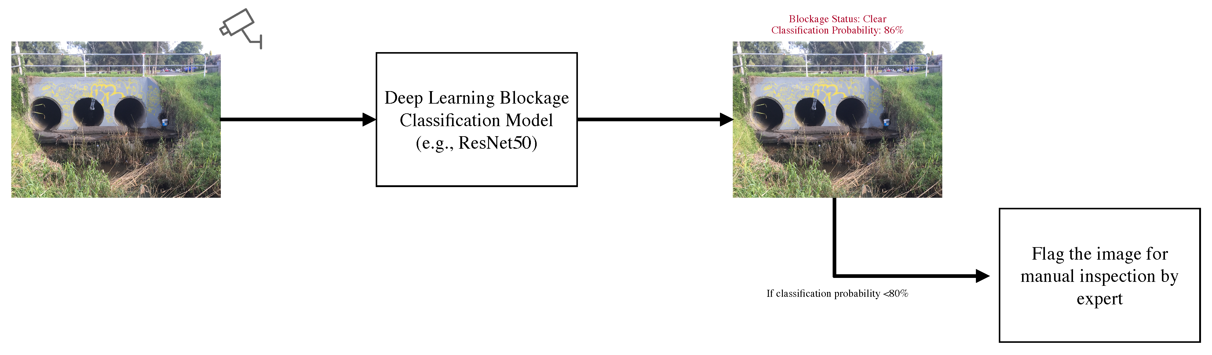
• Proposed a detection-classification pipeline to achieve higher blockage classification accuracy for practical implementation. Furthermore, a partial automation framework based on the class prediction probability is introduced using a single deep learning model to assist the visual inspection process.

The rest of the paper is organized as follows: Section 2 presents the theoretical background of the implemented CNN models in this investigation. Section 3 provides information about the dataset used in this study for culvert blockage classification. Section 4 outlines the experimental protocols adopted to perform the experiments. Furthermore, this section provides information about the evaluation measures used to assess the classification performance of the implemented models. Section 5 presents the results of the experiments and also reports the critical insights from the investigation. Section 6 presents a brief introduction to the detection-classification pipeline towards improving the blockage classification performance. Section 7 concludes the study and reports the highlighted outcomes from the experiments. Furthermore, the section lists potential future applications of the presented research.

2. Deep Learning Models

This section presents the theoretical background of the implemented deep learning models for culvert visual blockage classification. For the presented investigation, one model from each common and state of the art category of deep learning models was selected to demonstrate the diversity of applied approaches. A brief introduction, model concept, model architecture, and the fundamental mathematics is outlined for each model.

2.1. DarkNet53

Redmon and Farhadi [20] proposed you only look once (YOLOV3) in the year 2018, where they used DarkNet53 CNN architecture as the feature extractor. DarkNet53 is the variant of DarkNet19 (i.e., feature extractor CNN in YOLOV2) but with an increased number of convolutional layers and residual connections in between. The structure of the DarkNet53 model consists of successive $(3\times 3)$ and $(1\times 1)$ convolutional layers. DarkNet53 is much deeper than DarkNet19 and achieved better performance than DarkNet19, ResNet50, and ResNet102 for the ImageNet challenge. Model structure best utilizes the graphical processing unit (GPU), which makes it faster.

2.2. ResNet

He et al. [25] proposed a novel residual learning framework to facilitate the training of extremely deep networks. Rather than learning unreferenced functions, authors proposed the reformulation of layers as residual learning functions with reference to inputs of the layer. The residual learning concept helped in optimizing the deep networks and made it possible to achieve higher accuracy from deep models. Mathematically, let us say $H\left(x\right)$ denotes the desired mapping function, in residual learning, stacked non-linear layers fit another mapping function $F\left(x\right):=H\left(x\right)-x$. x denotes the inputs to the layer.

2.3. MobileNet

Howard et al. [24] proposed a category of CNN called MobileNets for cutting edge hardware applications with the idea of using depthwise separable convolutions towards building the deep networks. Two global hyperparameters were introduced to develop problem-specific models with accuracy and latency adjustments. Depthwise separable convolution is the type of factorized convolution that splits the standard convolution process of convolving and combining into two layers. At the first layer, depthwise convolution is performed, while at the second layer, a $1\times 1$ pointwise convolution is performed to combine the outputs from the depthwise convolution layer. All layers in the network are followed by a BatchNormalization and ReLu non-linearity. A depthwise convolution for a single filter per input channel can be expressed mathematically as in Equation (1).

$${\widehat{\mathbf{G}}}_{k,l,m}=\sum _{i,j}{\widehat{\mathbf{K}}}_{i,j,m}·{\mathbf{F}}_{k+i-1,l+j-1,m}$$

(1)

where $\widehat{\mathbf{K}}$ denotes the depthwise convolutional kernel, $\mathbf{F}$ denotes the feature map and $\widehat{\mathbf{G}}$ denotes the filtered output feature map.

2.4. InceptionV3 and InceptionResNet

Szegedy et al. [22,23] introduced the idea of inception module towards reducing the computational cost of the network without significantly affecting the generalized performance. InceptionV3 [23] and InceptionResNet [22] are improved versions of the proposed inception module. In InceptionV3, the idea of replacing large filters with small asymmetric filters was introduced and a $1\times 1$ convolution was used as a bottleneck before the large filters. Concurrent placement of $1\times 1$ filter resulted in cross-channel correlation. On the other hand, in the InceptionResNet model, Szegedy et al. [22] integrated both inception and residual concepts where concatenated filters were replaced by the residual connections. InceptionResNet was able to more quickly converge and achieved accelerated training performance.

2.5. VGG16

Simonyan and Zisserman [26] investigated the performance of deep convolutional networks by making architectural changes. The main idea was to replace the higher dimension filters with $3\times 3$ filters and increase the depth of the network. This resulted in improving the computational cost with a significantly smaller trade-off in accuracy. From experimental investigations, authors reported that smaller filters were able to induce similar features as larger dimension filters. Padding was used to maintain the spatial resolution. The idea of increasing the depth of the network with smaller resolution filters demonstrated significant success for large scale classification and localization tasks. However, an increase in depth to a large scale resulted in an increased number of trainable parameters.

2.6. DensNet121

Huang et al. [21] proposed densely connected convolutional networks called DenseNet by extending the concept of residual connections in the traditional networks. The authors proposed the idea of connecting each layer in the network to every other layer in the feedforward direction. This way, each layer will have the feature maps of all preceding layers at its input. In terms of the number of layer connections, a traditional network with L layers have L connections, while a densely connected convolutional network will have $L(L+1)/2$ connections. Densely connected networks have advantages including better feature propagation, feature reuse, a significant reduction in the number of network parameters, and improving the vanishing-gradient problem. A key difference between residual networks and densely connected networks is that in a densely connected network, feature maps from preceding layers are combined by concatenation rather than summation before feeding it to the next layer.

Mathematically, if a network consists of L number of layers each with a non-linear transformation through a composite function $F_l$, the output $x_l$ for the densely connected layer can be represented as in Equation (2).

$$x_l=F_l\left([x_0,x_1,\dots ,x_{l-1}]\right)$$

(2)

where $[x_0,x_1,\dots ,x_{l-1}]$ denotes the concatenation of the feature maps from the previous layers.

2.7. NASNet

Zoph et al. [28] proposed a new category of convolutional networks called NASNet based on the idea of directly training the architecture over the desired dataset. In order to overcome the issue of computational cost for relatively larger datasets, authors proposed to search for an architectural building for a smaller dataset, often called proxy dataset and then transferring it to a larger dataset. The search space which enables the transfer from a smaller dataset to a larger dataset is referred to as NASNet search space inspired from neural architecture search (NAS) [29]. Furthermore, to improve the generalization of the NASNet model, the authors proposed a novel normalization approach called ScheduledDropPath. In NAS, a recurrent neural network (RNN) controller samples the child architectures, which are trained over proxy datasets and based on the training accuracy, the controller improves the architecture. The main contribution of this approach is the decoupling of architecture complexity from depth.

2.8. EfficientNet

Tan and Le [27] proposed a novel compound coefficient based scaling of deep neural networks. Based on this idea, a new category of networks called EfficientNet is introduced, which is built on NAS. The idea of uniformly scaling the model in all dimensions, including width, depth, and resolution, is implemented. Balanced scaling up of models resulted in higher accuracy. Mathematically, if the intention is to extend the computation power to $2^n$ times, a model can be scaled up in depth, width, and resolution as ${\alpha }^n$, ${\beta }^n$, and ${\gamma }^n$, respectively.

3. Dataset

The dataset used in this research consisted of images of culverts (i.e., blocked, clear) from three different sources (i.e., ICOB, VHD, SIC). Overall, the dataset consisted of 3848 images. Details about each subset of the dataset are presented as follows.

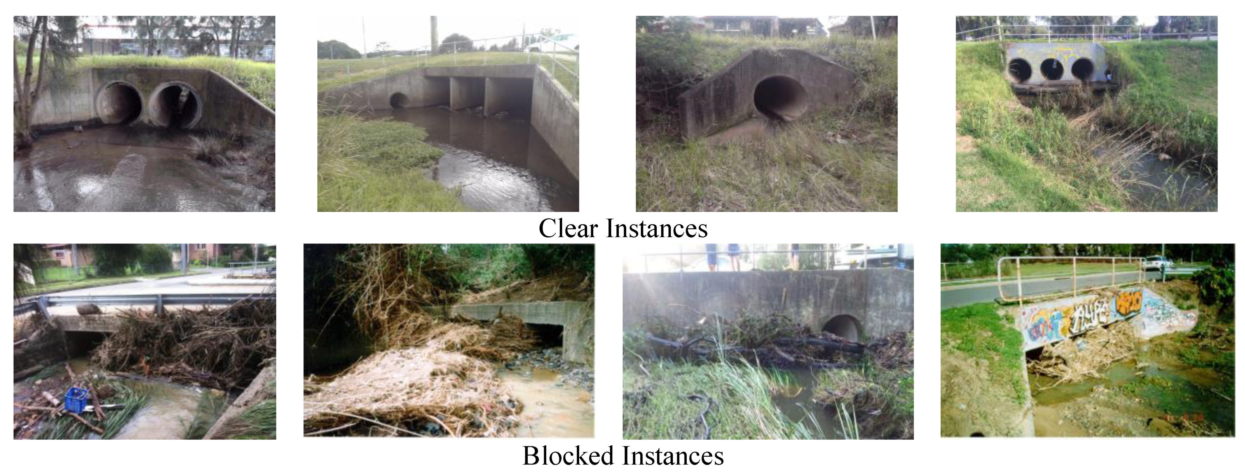
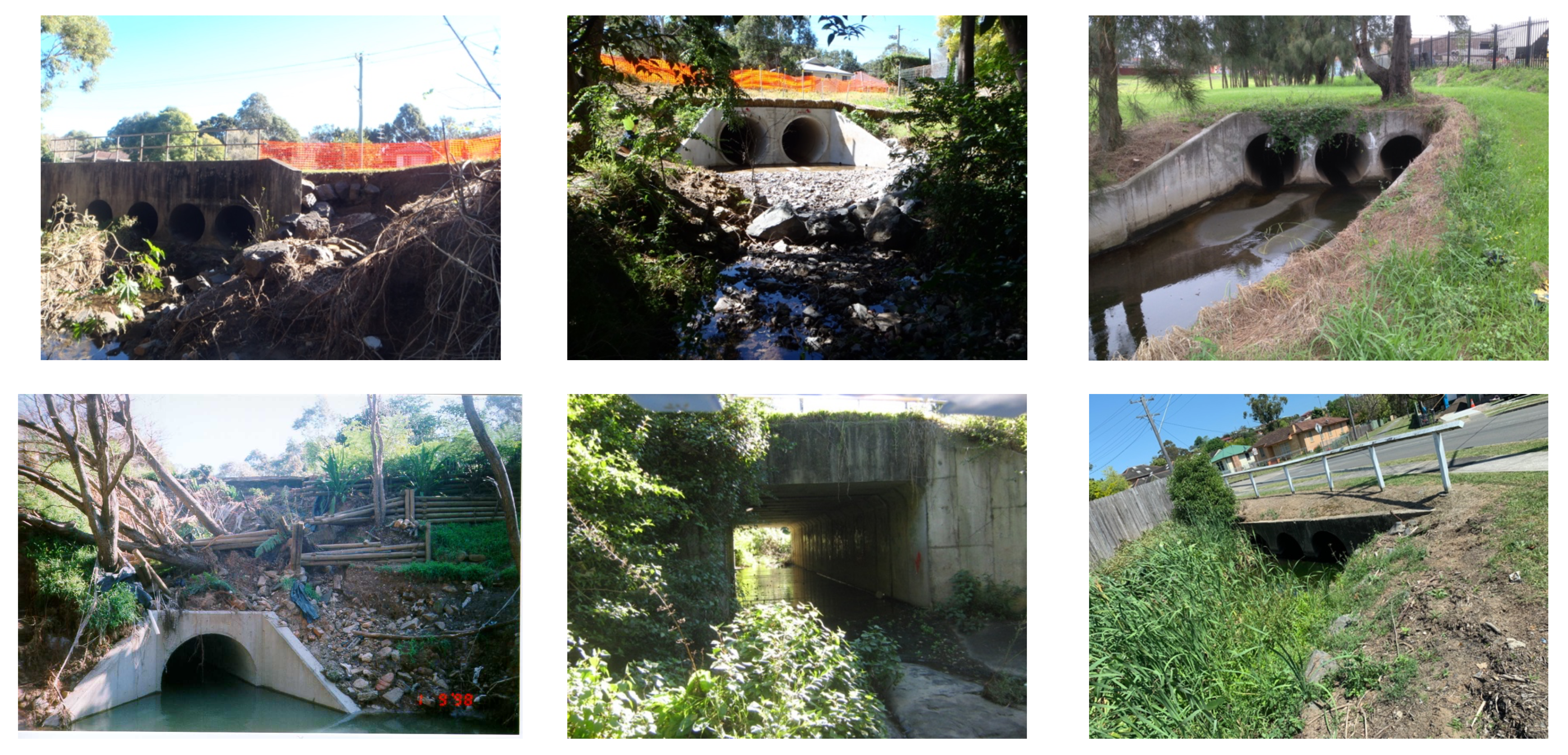
3.1. Images of Culvert Openings and Blockage (ICOB)

This dataset consisted of real images of culverts and referred to as “Images of Culvert Openings and Blockage (ICOB)”. Primary sources of images included WCC historical records, online records, and custom captured local culvert images. WCC records were scrutinized using a Microsoft ACCESS based application for filtering the culvert images with visible openings. The dataset contained images with a high level of variation from each other (intra-class variation) in terms of culvert types, blockage accumulation, presence of debris materials, illumination conditions, culvert viewpoint variations, scale variations, resolution, and backgrounds. This high level of diversity within a relatively small dataset makes it a challenging dataset for visual analysis, even for a binary classification problem. In total, there were 929 images in ICOB with 487 images in the “clear” class and 442 images in the “blocked” class. Figure 1 shows the sample instances from each class of ICOB.

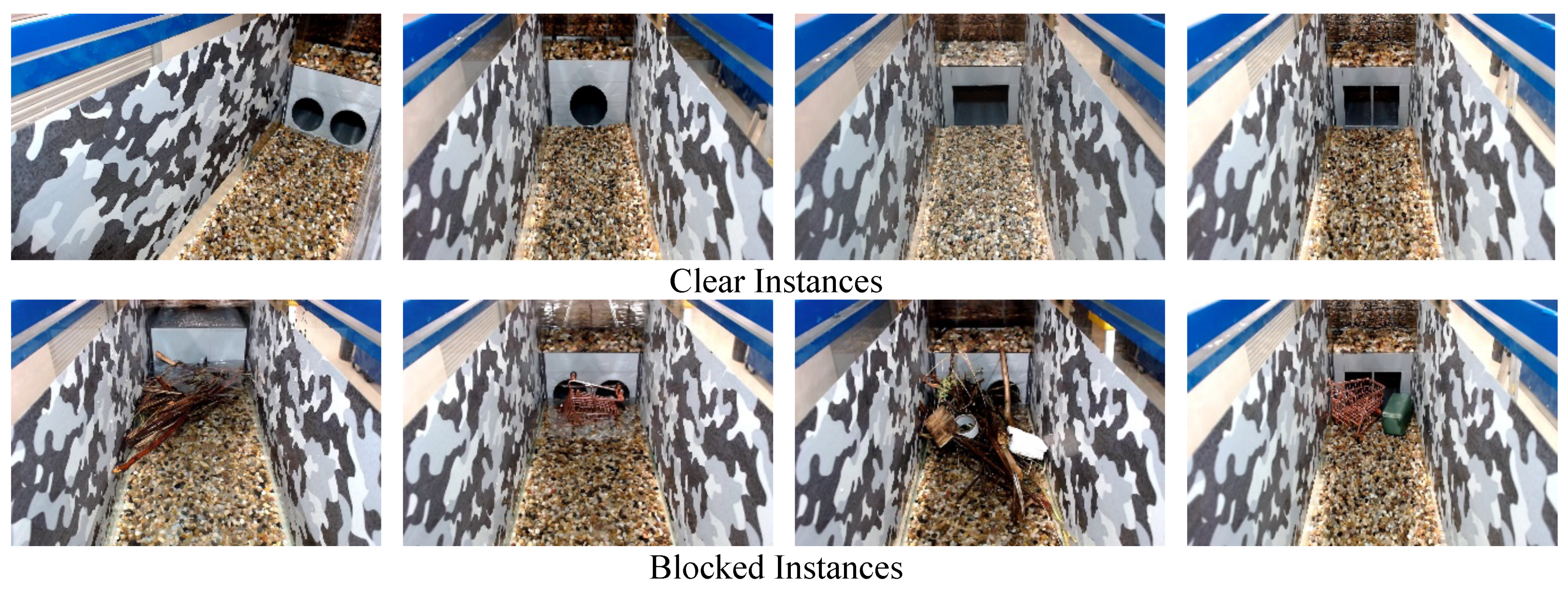
3.2. Visual Hydrology-Lab Dataset (VHD)

This dataset consisted of simulated images of culverts captured from a controlled hydrology lab experiment. A comprehensive in-lab investigation of blockage of carried out by performing series of experiments using scaled physical models of culverts under multiple flooding conditions. Experiments were recorded using two high definition (HD) cameras with a different view of the culvert and images of culverts in blockage and clear condition were extracted, referred to as “Visual Hydrology-Lab Dataset (VHD)”. VHD consisted of a diversity of images including four different culvert configurations (i.e., single circular, double circular, single box, double box), different blockage types (i.e., urban, vegetative, mixed), different simulated lighting conditions, different camera viewpoints, and different flood levels controlled by inlet water discharge. Limitations of the dataset included reflections from the water surface and flume walls, identical background and scaling, and clear water. For this investigation, in total, 1630 images were used with 1526 images from the “blocked” class while 104 images from the “clear” class. Figure 2 shows the sample images of each class from VHD.

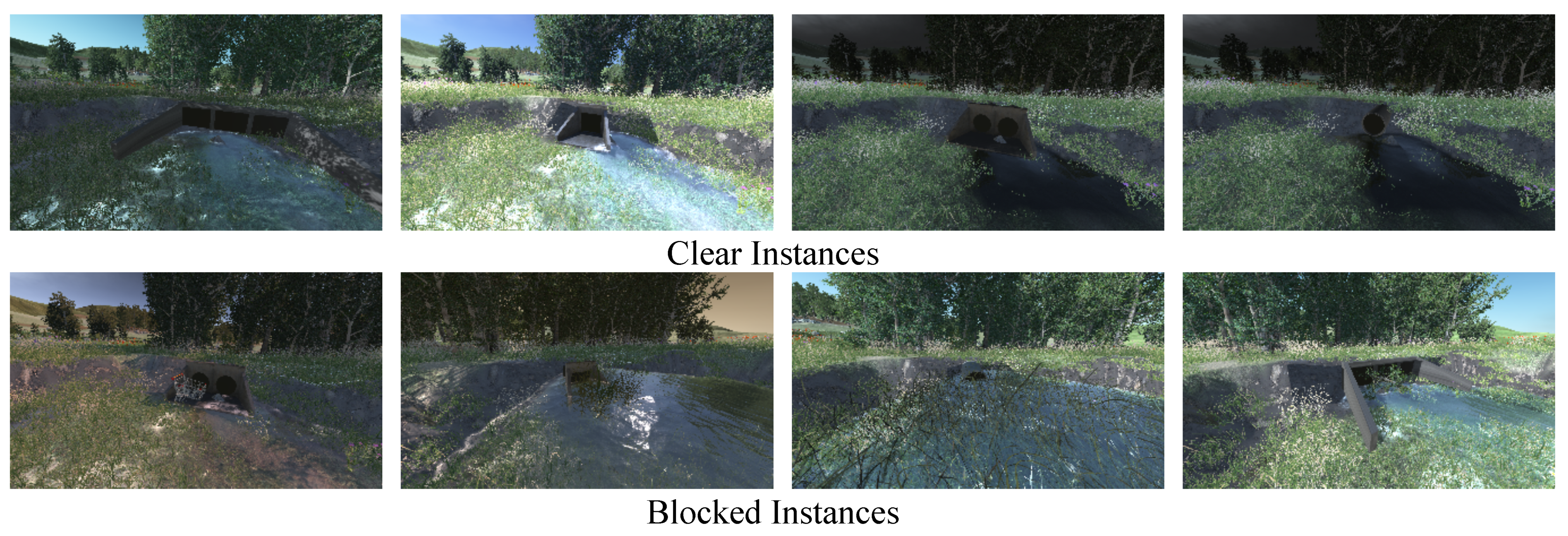
3.3. Synthetic Images of Culverts (SIC)

This dataset consisted of synthetic images of culverts generated using a three-dimensional (3D) computer application based on a gaming engine (i.e., Unity3D) specifically designed to simulate multiple culvert blockage scenarios. Application has the capability to generate virtually countless blockage scenarios by dragging different debris materials into the scene and placing them in desired orientation/location. Images of different simulated blockage scenarios were captured using batch capture functionality and are referred to as “Synthetic Images of Culvert (SIC)”. Dataset offered the diversity in terms of debris type (i.e., urban, vegetative, mixed), culvert types (i.e., pipe, single circular, double circular, single box, double box, triple box), camera viewpoints, time of day, and water levels. Limitations of the dataset include single natural background and non-realistic effects/animations. For this investigation, 1289 images were used with 1140 images from the “blocked” class while 149 images from the “clear” class. Figure 3 shows the sample images of each class from SIC.

3.4. Labeling Criteria

Dataset was manually labeled for binary classification of a given image with culvert as “clear” or “blocked”. A culvert being visually blocked or clear is not as simple and may require defining detailed criteria in collaboration with flood management officers; however, for this article, simple occlusion based criteria was used. Following subjective annotation criteria was used for labeling.

• If all of the culvert openings are visible, classify it as “clear”;
• If any of the culvert openings is visually occluded by debris material or foreground object (e.g., debris control structure, vegetation, tree), classify it as “blocked”.

4. Experimental Setup and Evaluation Measures

Experiments were planned to investigate the performance of existing CNN models for binary classification of culvert images as blocked or clear. Pre-trained CNN models with ImageNet weights were used for this investigation and implemented using Keras with Tensorflow at the backend. Images of dimension $224\times 224\times 3$ were used as input to model except for NASNet where $331\times 331\times 3$ and InceptionResNetV2 where $229\times 229\times 3$ was used. Data augmentations techniques including samplewise standard deviation normalization, horizontal flip, vertical flip, rotation, width shift, and height shift were used in the simulations for improved performance. All the models were tuned with a dropout of 0.2, ReLU activation, and batch normalization. Stochastic gradient descent (SGD) optimizer with a constant learning rate of 0.01 and categorical entropy loss was used. Each model was trained for 30 epochs. For this investigation, the test dataset consisted of selected real images from ICOB (i.e., 91 from blocked, 98 from clear). The rest of the dataset was divided using conventional train:val split with an 80:20 ratio. In addition to the conventional train:val:test dataset split, the 5-fold cross-validation approach has also been implemented and compared towards providing better insight into the performance of deep learning models. The idea of classifying deep visual features extracted from CNN models using conventional machine learning approaches was also implemented. The simulations were performed using Nvidia GeForce RTX 2060 GPU with 6 GB memory and 14 Gbps memory speed. Models were trained at full precision using floating point (FP-32) optimization.

The performance of the models was measured in terms of their test accuracy, test loss, precision score, recall score, F1 score, Jaccard Index, ROC curves, and processing times. Each of the evaluation metrics is defined briefly as follows.

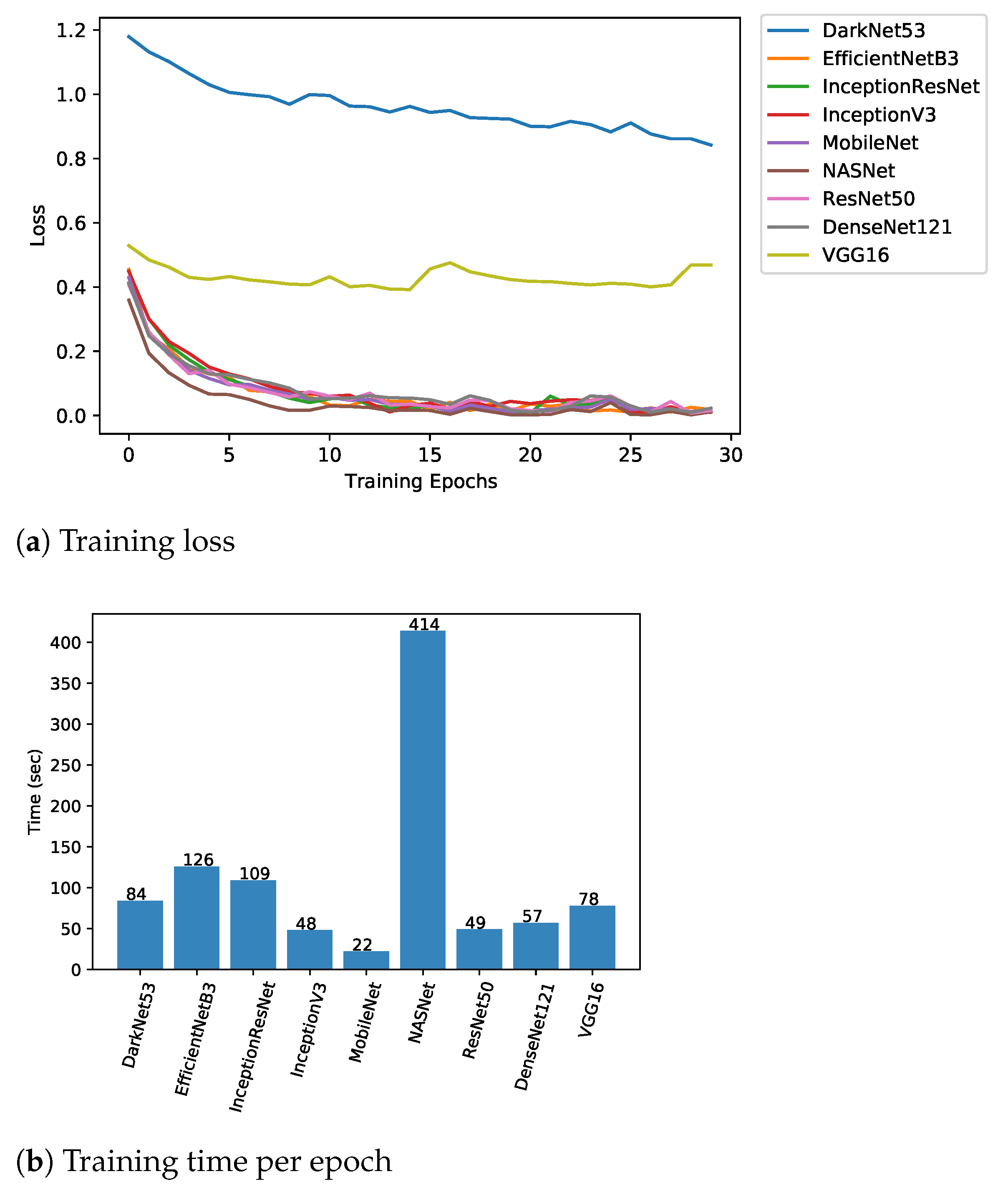
• Loss: Loss is the simplest of the measure to evaluate model training and testing performance. It is the measure of how much instances are classified incorrectly and is the ratio of number of incorrect predictions over total predictions. Minimum value of loss indicated better performance;
• Accuracy: In contrast to loss, accuracy is the measure that how much percentage of data instances are classified correctly. It is the ratio of number of correct predictions over total predictions. High value of accuracy represents better performance;
• Precision Score: Precision measures the ability of a model to not to classify a negative instance as positive. It answers the question that from all the positive predicted instances by model, how many were actually positive. The equation below presents the expression for the precision score:

  $$\mathrm{Precision}\mathrm{Score}=\frac{\mathrm{True}\mathrm{Positive}\left(\mathrm{TP}\right)}{\mathrm{True}\mathrm{Positive}\left(\mathrm{TP}\right)+\mathrm{False}\mathrm{Positive}\left(\mathrm{FP}\right)}$$
• Recall Score: Recall answers the question that from all the positive instances, how many were correctly classified by the model. Expression for recall score is given as follows:

  $$\mathrm{Recall}\mathrm{Score}=\frac{\mathrm{True}\mathrm{Positive}\left(\mathrm{TP}\right)}{\mathrm{True}\mathrm{Positive}\left(\mathrm{TP}\right)+\mathrm{False}\mathrm{Negative}\left(\mathrm{FN}\right)}$$
• F1 Score: F1 score is the single measure which combines both precision and recall by harmonic mean and range between 0 and 1. Higher F1 score indicates the better performance of model. Expression for F1 score is given as follows:

  $$\mathrm{F}1\mathrm{Score}=2\times \frac{\mathrm{Precision}\times \mathrm{Recall}}{\mathrm{Precision}+\mathrm{Recall}}$$
• Jaccard Index: In context of classification, Jaccard similarity index score measures the similarity between predicted labels and actual labels. Mathematically, let $\widehat{y}$ denotes the predicted label and y denotes the actual label, then J index can be expressed as follows. Higher J index indicates better performance of model.

  $$\mathrm{Jaccard}\mathrm{Index}=\frac{|\widehat{y}\cap y|}{|\widehat{y}\cup y|}=\frac{|\widehat{y}\cap y|}{|\widehat{y}|+|y|-|\widehat{y}\cap y|}$$

In addition, confusion matrices were plotted to assess the Type I and Type II errors. Type I (False positive (FP)) and Type II (False negative (FN)) errors [30] are commonly used terms in machine learning and the main goal of the model is to minimize one of these two errors, depending on the context that which error is more critical in the given task. By definition, a Type I error is concluding the existence of a relationship, while in fact it does not exist (e.g., classifying an image as “blocked” while there is no blockage). Similarly, a Type II error is the rejection of the existence of relationship while, in fact, it exists (e.g., classifying an image as “clear” while there is a blockage). For the given culvert blockage context, Type II error is more critical to be minimized in comparison to Type I error because having notified as blocked while there is no blockage is tolerable in comparison to having notified as clear while there is a blockage. Type II error will result in damages because it may be very late for the response team to clear the blockage before the diversion of flow. Finally, the performance of implemented deep learning models was benchmarked against the conventional machine learning models (i.e., SVM, RF, xgboost) to demonstrate the effectiveness of CNN’s for images (i.e., matrix) type dataset.

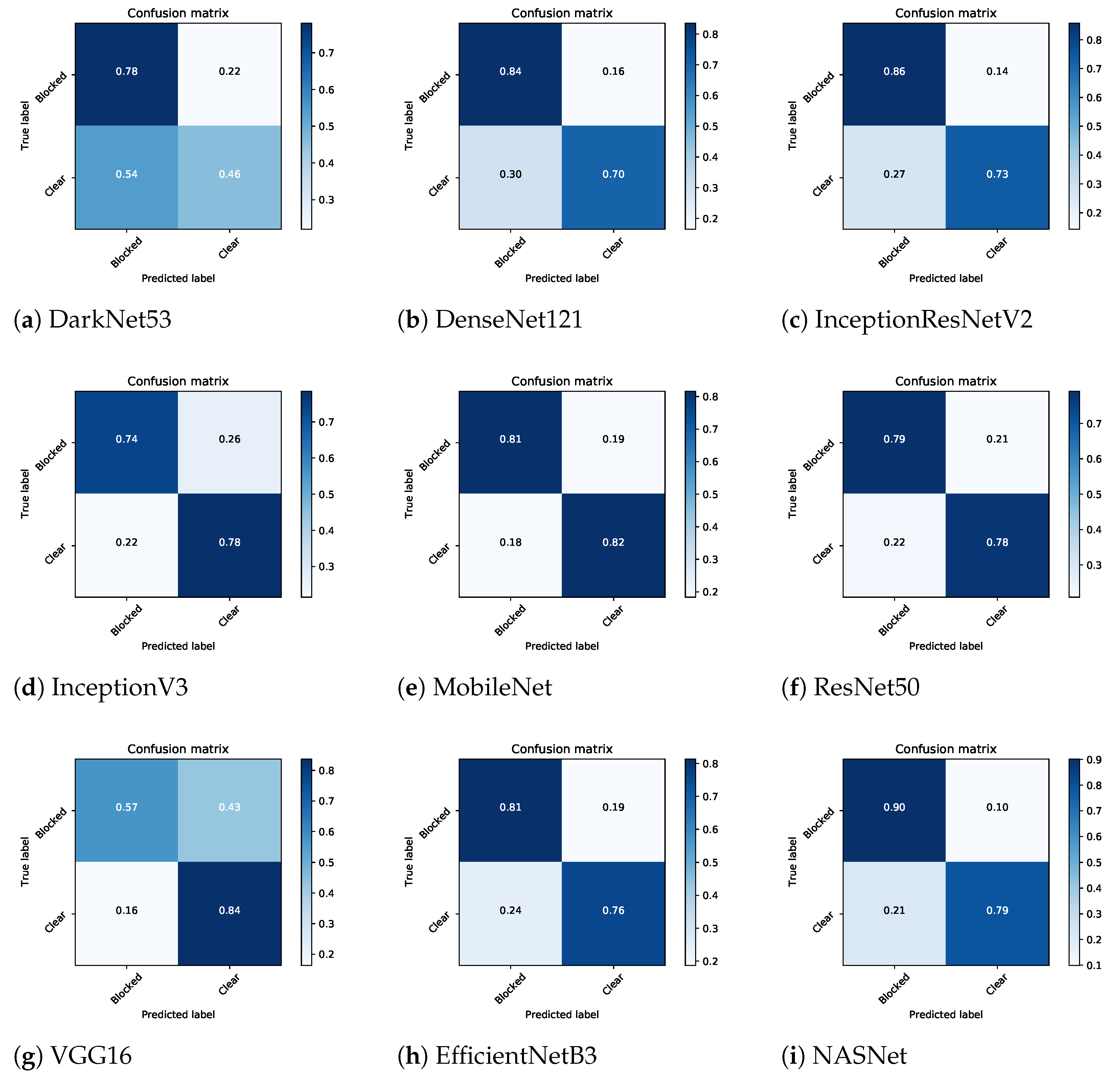
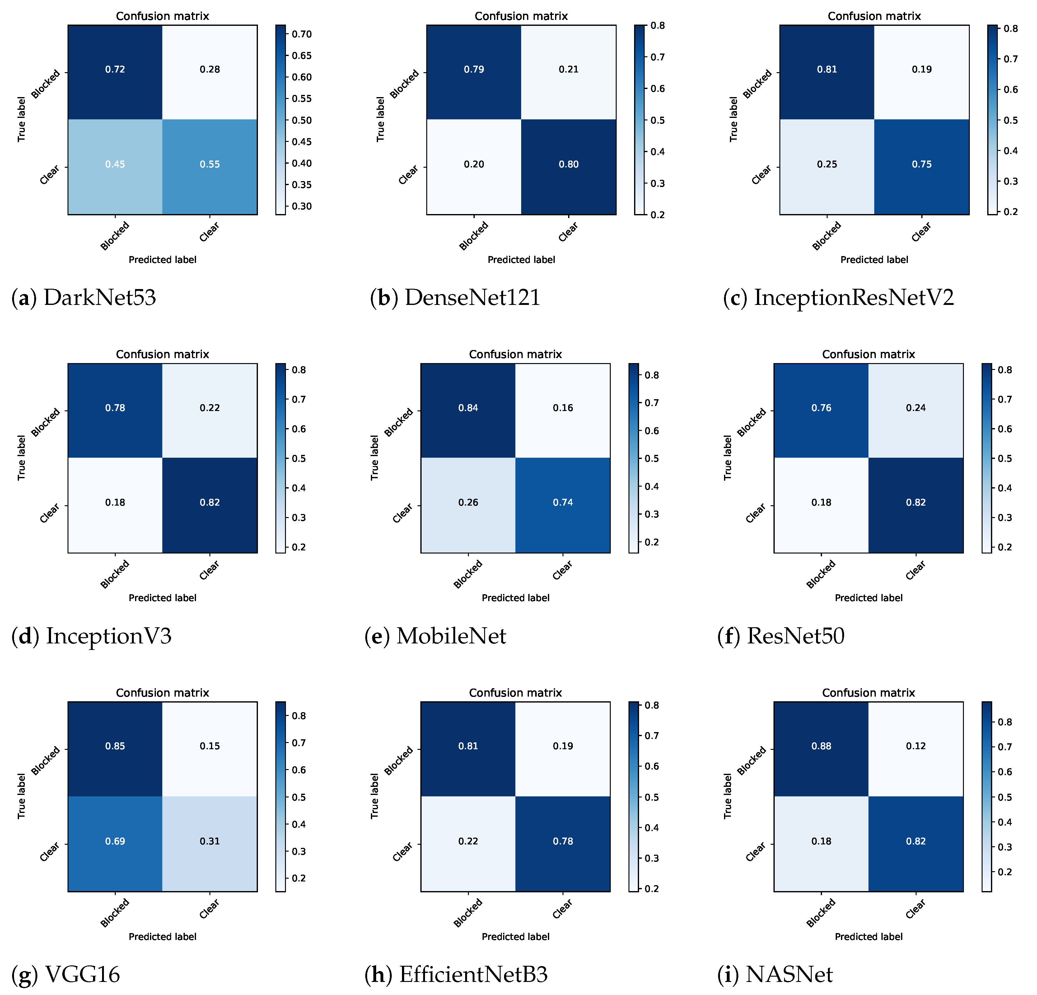
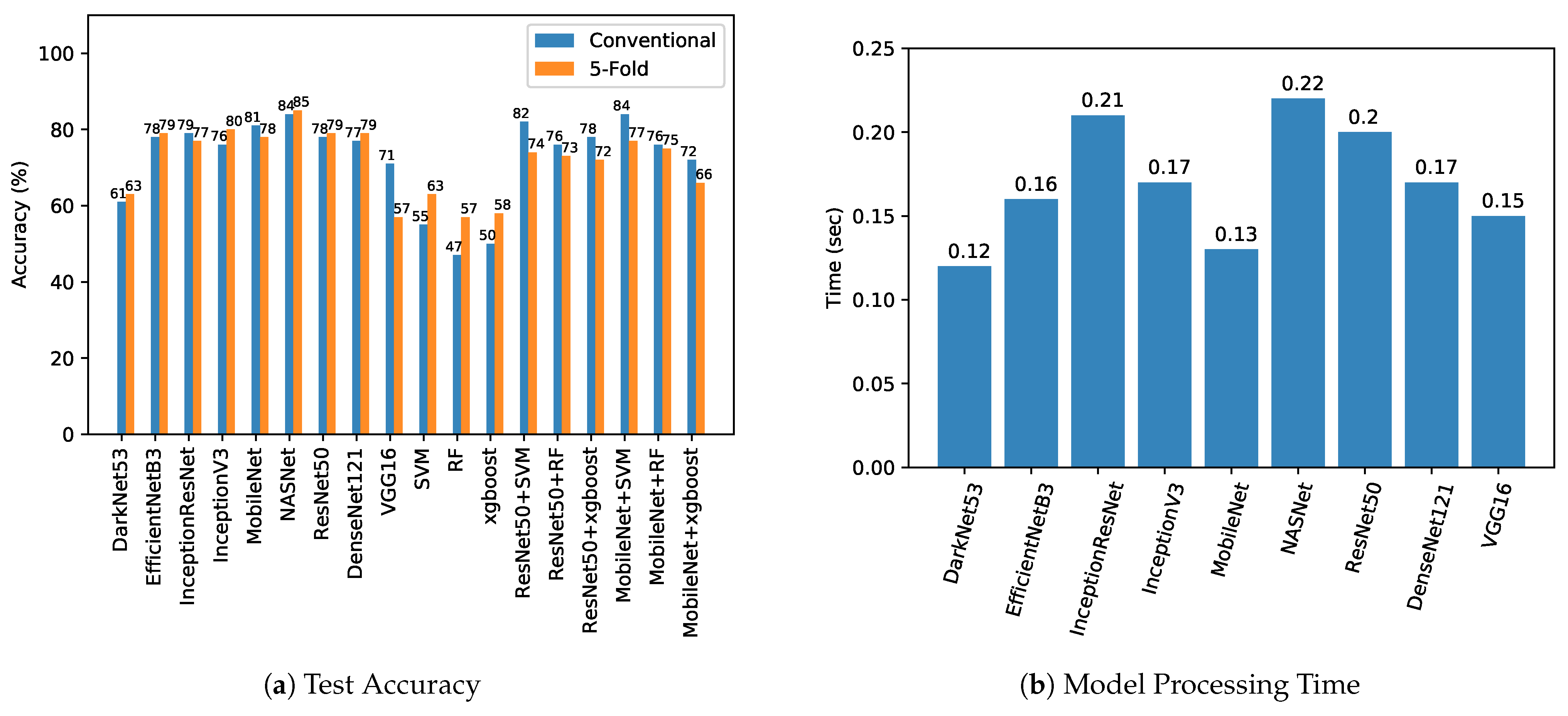
5. Results and Discussion

Implemented CNN models were evaluated as per defined measures in Section 4 and results were compared. Figure 4 shows the training performance of implemented models in terms of training loss for conventional dataset split and the training times. From the figure, it can be observed that other than the DarkNet53 and VGG16, all models training behaviour was similar with loss following the negative exponential curve and converging to a minimum value. However, unusual training behavior was observed for DarkNet53 and VGG16 where models failed to learn the training examples and loss did not decrease significantly over the training epochs. In terms of training times, as expected NASNet was the slowest to train (i.e., 414 s per epoch), while MobileNet was the fastest to train (i.e., 22 s per epoch) based on their respective complexity.

Table 1. Classification performance of implemented artificial intelligence models for visual blockage detection.

	Test Accuracy		Test Loss/Log Loss		Precision Score		Recall Score		F1 Score		Jaccard Index		FLOPs
	Conventional	5-Fold	Conventional	5-Fold	Conventional	5-Fold	Conventional	5-Fold	Conventional	5-Fold	Conventional	5-Fold
Deep Learning Models
DarkNet53	0.61	0.63	1.20	1.21	0.63	0.65	0.62	0.61	0.61	0.61	0.44	0.46	14.2 G
DenseNet121	0.77	0.79	0.47	0.57	0.77	0.80	0.77	0.79	0.77	0.79	0.62	0.66	5.7 G
InceptionResNetV2	0.79	0.77	0.58	0.65	0.79	0.78	0.80	0.78	0.80	0.77	0.66	0.64	13.3 G
InceptionV3	0.76	0.80	0.74	0.64	0.76	0.80	0.76	0.80	0.76	0.80	0.62	0.66	5.69 G
MobileNet	0.81	0.78	0.51	0.59	0.81	0.79	0.81	0.79	0.81	0.78	0.69	0.65	1.15 G
ResNet50	0.78	0.79	0.70	0.62	0.78	0.76	0.78	0.76	0.78	0.79	0.64	0.65	7.75 G
VGG16	0.71	0.57	0.58	0.79	0.72	0.43	0.70	0.58	0.70	0.48	0.55	0.41	30.7 G
EfficientNetB3	0.78	0.79	0.46	0.57	0.78	0.80	0.78	0.79	0.78	0.79	0.64	0.66	1.97 G
NASNet	0.84	0.85	0.58	0.55	0.85	0.85	0.84	0.85	0.84	0.85	0.73	0.73	47.8 G
Conventional Machine Learning Algorithms
SVM	0.55	0.63	15.53	12.61	0.70	0.64	0.57	0.63	0.46	0.63	0.38	0.47	NA
RF	0.47	0.57	18.27	14.80	0.47	0.57	0.48	0.57	0.40	0.56	0.31	0.40	NA
xgboost	0.50	0.58	17.18	14.62	0.58	0.58	0.52	0.57	0.40	0.57	0.34	0.41	NA
Deep CNN Visual Features Classification using Conventional Machine Learning Approaches
ResNet50 Features + SVM	0.82	0.74	6.31	9.11	0.82	0.74	0.82	0.74	0.82	0.74	0.69	0.58	NA
ResNet50 Features + RF	0.76	0.73	8.24	9.29	0.78	0.73	0.76	0.73	0.76	0.73	0.61	0.58	NA
ResNet50 Features + xgboost	0.78	0.72	7.36	9.64	0.79	0.72	0.79	0.72	0.79	0.72	0.65	0.56	NA
MobileNet Feature + SVM	0.84	0.77	5.25	7.88	0.85	0.77	0.85	0.77	0.85	0.77	0.74	0.63	NA
MobileNet Feature + RF	0.76	0.75	8.06	8.41	0.77	0.78	0.77	0.76	0.77	0.75	0.62	0.61	NA
MobileNet Feature + xgboost	0.72	0.66	9.64	11.74	0.73	0.66	0.72	0.66	0.72	0.66	0.56	0.49	NA

presents the empirical results of all implemented models using conventional dataset split and 5-fold cross-validation when evaluated for test dataset in terms of accuracy, loss, precision, recall, F1 score, and Jaccard Index. Furthermore, the table benchmarks the results of deep learning models against conventional machine learning algorithms. From the results, NASNet was reported as the best among all others with an F1 score of 0.84 and 0.85 for conventional and 5-fold, respectively. MobileNet was reported as the second-best for conventional dataset split with an F1 score of 0.81, while InceptionV3 was reported second best for 5-fold with an F1 score of 0.80. DarkNet and VGG performed worst with the F1 scores of 0.61 and 0.48 for 5-fold cross-validation. When benchmarked against the conventional machine learning algorithms, it can be clearly observed that deep learning models performed significantly better. However, for the case where the idea of classifying deep visual features using conventional machine learning models, comparable performance to standard CNN models was achieved. 5-fold accuracy of 77% was achieved as best for the case where MobileNet extracted visual features were classified using an SVM conventional machine learning classifier.

Performance of deep learning models was also assessed using ROC curves as given in Figure 5. ROC plot confirmed that NASNet outperformed other models with an area under the curve (auc) of 0.92. Figure 6 and Figure 7 show the confusion matrices for both conventional and 5-fold cross-validation experiments, respectively, to observe the Type I and Type II errors. For the conventional case presented in Figure 6, it can be observed that NASNet performed best in terms of the lowest Type II error of the only 10%; however, Type I error was reported 21%. On the other hand, MobileNet was reported with balanced Type I and Type II errors (19% and 18%). A similar trend was observed for the 5-fold cross-validation experiment where NASNet was reported with the lowest Type II error (i.e., 12%) and EfficientNetB3 was reported balanced Type I and Type II errors (19% and 22%). Overall, comparatively similar performance was reported for both conventional and 5-fold experiments except for the case of VGG where 5-fold cross-validation performance was degraded significantly (see Figure 8a).

From the FP instances in Figure 9, it was observed that for the cases where there are more than two openings and only one opening was blocked, the algorithm classified it as clear. This insight led to a suggestion in the change of labeling criteria. A better approach could be to label the image as blocked if half or more than half of the openings are blocked; otherwise, label it as clear. Furthermore, if there is no debris material present in the image and occlusion is due to some foreground object not similar to debris in visual appearance, the image should be labeled as clear. From the FN instances in Figure 9, it was observed that for the cases where the image contained contents with a visual appearance similar to blockage material, the image was classified as blocked. This indicated the existence of background clutter/noise problems for this investigation. Background clutter hypothesis was also verified by the intermediate CNN layers activation and heatmaps as given in Figure 10 and Figure 11, respectively. From the layers intermediate activation, it can be observed that at the initial layer, the model retained almost all the visual information as in the input image. However, as the layers go deeper, the model tends to encode higher-level features, such as borders, lines, and edges. Going further deeper results in activation which are not visually interpretable and possess more information related to the class of the input image. Heatmaps for selected FN cases presented in Figure 11 confirmed the hypothesis of background clutter. It can be observed that in most cases, the focus was more on the background contents rather than the culvert opening. Interestingly, in the case of the box culvert, the reflection of light through the culvert was considered by the model as the background which resulted in false classification.

Given that, existing CNN models, conventional machine learning approaches, and classification of deep CNN visual features using conventional machine learning approaches did not achieve high enough accuracy (i.e., maximum 5-fold accuracy of 85% achieved for NASNet model) that they can be deployed to replace the manual visual inspection of culverts. However, they can potentially be used to partially automate the process of manual visual inspection of culverts. Along with the predicted blockage class of a given culvert (i.e., blocked, clear), the value of class prediction probability can help in estimating the model confidence of the prediction. Partial automation can be achieved by setting a threshold on prediction probability (i.e., 80%) to filter only those images for manual inspection for which prediction probability is less than a set threshold. Figure 12 shows the conceptual block diagram of the proposed framework for partial automation of the culvert visual blockage inspection process.

Implemented CNN models were also compared for their processing times to investigate the relative response times. The purpose of these analyses was to investigate the hardware implementability of proposed models for real-world applications. Model inference time and image processing time were calculated as two measures to compare the models. Three different size images were used; image 1 of $2048\times 1536$, image 2 of $3264\times 2448$, and image 3 of $4032\times 3024$. From

Table 2. CNN model processing times for three different size images.

	Model Processing Time (s)	Total Execution Time (s)
		Image 1	Image 2	Image 3
DarkNet53	0.05	0.12	0.2	0.35
DenseNet121	0.09	0.17	0.24	0.39
InceptionResNetV2	0.14	0.21	0.29	0.44
InceptionV3	0.09	0.17	0.24	0.39
MobileNet	0.06	0.13	0.21	0.36
ResNet152	0.13	0.20	0.28	0.43
ResNet50	0.08	0.15	0.23	0.38
VGG16	0.08	0.15	0.23	0.38
EfficientNetB3	0.09	0.16	0.24	0.39
NASNet	0.15	0.22	0.30	0.45

and Figure 8, it can be observed that MobileNet and DarkNet53 were fastest among others while the NASNet model was the slowest. In terms of accuracy, NASNet was the most accurate; however, MobileNet also exhibited comparatively good accuracy (i.e., 78% in comparison to 85% for NASNet) and was recommended as a suitable choice to implement for on-board processing. Figure 8 shows the graphical comparison of implemented models in terms of test accuracy and processing times. It is important to mention that reported processing times are for relative comparison between models and not the actual measure of cutting edge hardware performance. However, given the availability of efficient computing hardware, such as Nvidia Jetson TX2 [31] and Nvidia Jetson Nano [32], it is highly probable to implement any of the implemented models for real-world applications (e.g., pedestrian detection [33], wildlife tracking [34]).

6. Detection-Classification Pipeline for Visual Blockage Detection

In light of the reported insights from the presented experiments in Section 5, a detection-classification pipeline is a potential future work in the development process to address the background clutter issue. The idea is to detect the culvert openings from the image using the object detection model (i.e., Faster R-CNN [35]) at the first stage and classify the detected culvert openings as “blocked” or “clear” using a deep learning classification model (i.e., ResNet50). Figure 13 shows the conceptual block diagram of the detection-classification pipeline. A preliminary system with such a pipeline has already been deployed on a cutting edge hardware for testing purposes [18]. For culvert opening detection, m@AP50 of 0.95 has been achieved using the Faster R-CNN model while an improved 94% blockage classification accuracy has been achieved using the ResNet50 model.

7. Conclusions and Future Directions

The idea of using visual analytic for the culvert blockage analysis has been successfully pitched by implementing existing CNN models for culvert blockage classification. Dataset from three different sources (i.e., ICOB, VHD, SIC) has been developed with a diversity of clear and blocked culvert instances for training the convolutional neural network (CNN) models. From the analysis, it has been observed that the NASNet model performed best among all in terms of classification performance; however, it was the slowest in relative comparison of processing times. Based on the classification performance and processing times, MobileNet was recommended model to be deployed for real-world applications. Deep learning models were benchmarked against conventional machine learning algorithms and reported significantly improved performance. From the false positive (FP) and false negative (FN) instances, background noise and oversimplified labeling criteria were found potential factors for degraded performance. A detection-classification pipeline was proposed with higher blockage classification accuracy (i.e., 94%) as a potential solution for real-world implementation. Furthermore, a partial automation framework based on the model class prediction probability was introduced to facilitate the manual visual inspections of culverts. A visual attention based approach and problem-specific CNN design are potential future directions of this research. Furthermore, study the impact of high-resolution images on the accuracy and developing a hybrid model taking into account information from multiple sensors are the potential concepts that can be investigated in future.

References

1. French, R.; Jones, M. Culvert blockages in two Australian flood events and implications for design. Australas. J. Water Resour. 2015, 19, 134–142. [Google Scholar] [CrossRef]
2. French, R.; Rigby, E.; Barthelmess, A. The non-impact of debris blockages on the August 1998 Wollongong flooding. Australas. J. Water Resour. 2012, 15, 161–169. [Google Scholar] [CrossRef]
3. Blanc, J. An Analysis of the Impact of Trash Screen Design on Debris Related Blockage at Culvert Inlets. Ph.D. Thesis, School of the Built Environment, Heriot-Watt University, Edinburgh, UK, 2013. [Google Scholar]
4. Weeks, W.; Witheridge, G.; Rigby, E.; Barthelmess, A.; O’Loughlin, G. Project 11: Blockage of Hydraulic Structures; Technical Report P11/S2/021; Engineers Australia, Water Engineering: Barton, ACT, Australia, 2013. [Google Scholar]
5. Roso, S.; Boyd, M.; Rigby, E.; VanDrie, R. Prediction of increased flooding in urban catchments due to debris blockage and flow diversions. In Proceedings of the 5th International Conference on Sustainable Techniques and Strategies in Urban Water Management (NOVATECH), Lyon, France, 6–10 June 2004; Water Science and Technology: Lyon, France, 2004; pp. 8–13. [Google Scholar]
6. Wallerstein, N.; Thorne, C.R.; Abt, S. Debris Control at Hydraulic Structures, Contract Modification: Management of Woody Debris in Natural Channels and at Hydraulic Structures; Technical Report; Department of Geography, Nottingham University (United Kingdom): Nottingham, UK, 1996. [Google Scholar]
7. Iqbal, U.; Perez, P.; Li, W.; Barthelemy, J. How Computer Vision can Facilitate Flood Management: A Systematic Review. Int. J. Disaster Risk Reduct. 2021, 53, 102030. [Google Scholar] [CrossRef]
8. Barthelmess, A.; Rigby, E. Culvert Blockage Mechanisms and their Impact on Flood Behaviour. In Proceedings of the 34th World Congress of the International Association for Hydro-Environment Research and Engineering, Brisbane, Australia, 26 June–1 July 2011; Engineers Australia: Barton, ACT, Australia, 2011; pp. 380–387. [Google Scholar]
9. Rigby, E.; Silveri, P. Causes and effects of culvert blockage during large storms. In Proceedings of the Ninth International Conference on Urban Drainage (9ICUD), Portland, OR, USA, 8–13 September 2002; Engineers Australia: Portland, OR, USA, 2002; pp. 1–16. [Google Scholar]
10. Van Drie, R.; Boyd, M.; Rigby, E. Modelling of hydraulic flood flows using WBNM2001. In Proceedings of the 6th Conference on Hydraulics in Civil Engineering, Hobart, Australia, 28–30 November 2001; Institution of Engineers Australia: Hobart, Australia, 2001; pp. 523–531. [Google Scholar]
11. Davis, A. An Analysis of the Effects of Debris Caught at Various Points of Major Catchments during Wollongong’s August 1998 Storm Event. Bachelor’s Thesis, University of Wollongong, Wollongong, Australia, 2001. [Google Scholar]
12. WBM, B. Newcastle Flash Flood 8 June 2007 (the Pasha Bulker Storm) Flood Data Compendium; Prepared for Newcastle City Council; BMT WBM: Broadmeadow, Australia, 2008. [Google Scholar]
13. Ball, J.; Babister, M.; Nathan, R.; Weinmann, P.; Weeks, W.; Retallick, M.; Testoni, I. Australian Rainfall and Runoff—A Guide to Flood Estimation; Commonwealth of Australia: Barton, ACT, Australia, 2016. [Google Scholar]
14. French, R.; Jones, M. Design for culvert blockage: The ARR 2016 guidelines. Australas. J. Water Resour. 2018, 22, 84–87. [Google Scholar] [CrossRef]
15. Rigby, E.; Silveri, P. The impact of blockages on flood behaviour in the Wollongong storm of August 1998. In Proceedings of the 6th Conference on Hydraulics in Civil Engineering: The State of Hydraulics, Hobart, Australia, 28–30 November 2001; Engineers Australia: Barton, ACT, Australia, 2001; pp. 107–115. [Google Scholar]
16. Ollett, P.; Syme, B.; Ryan, P. Australian Rainfall and Runoff guidance on blockage of hydraulic structures: Numerical implementation and three case studies. J. Hydrol. 2017, 56, 109–122. [Google Scholar]
17. Jones, R.H.; Weeks, W.; Babister, M. Review of Conduit Blockage Policy Summary Report; WMA Water: Sydney, NSW, Australia, 2016. [Google Scholar]
18. Barthelemy, J.; Amirghasemi, M.; Arshad, B.; Fay, C.; Forehead, H.; Hutchison, N.; Iqbal, U.; Li, Y.; Qian, Y.; Perez, P. Problem-Driven and Technology-Enabled Solutions for Safer Communities: The case of stormwater management in the Illawarra-Shoalhaven region (NSW, Australia). In Handbook of Smart Cities; Augusto, J.C., Ed.; Springer: Berlin, Germany, 2020; pp. 1–28. [Google Scholar]
19. Arshad, B.; Ogie, R.; Barthelemy, J.; Pradhan, B.; Verstaevel, N.; Perez, P. Computer Vision and IoT-Based Sensors in Flood Monitoring and Mapping: A Systematic Review. Sensors 2019, 19, 5012. [Google Scholar] [CrossRef] [PubMed] [Green Version]
20. Redmon, J.; Farhadi, A. Yolov3: An incremental improvement. arXiv 2018, arXiv:1804.02767. [Google Scholar]
21. Huang, G.; Liu, Z.; Van Der Maaten, L.; Weinberger, K.Q. Densely connected convolutional networks. In Proceedings of the IEEE Conference on Computer Vision and Pattern Recognition, Honolulu, HI, USA, 21–26 July 2017; pp. 4700–4708. [Google Scholar]
22. Szegedy, C.; Ioffe, S.; Vanhoucke, V.; Alemi, A. Inception-v4, inception-resnet and the impact of residual connections on learning. arXiv 2016, arXiv:1602.07261. [Google Scholar]
23. Szegedy, C.; Vanhoucke, V.; Ioffe, S.; Shlens, J.; Wojna, Z. Rethinking the inception architecture for computer vision. In Proceedings of the IEEE Conference on Computer Vision and Pattern Recognition, Las Vegas, NV, USA, 27–30 June 2016; pp. 2818–2826. [Google Scholar]
24. Howard, A.G.; Zhu, M.; Chen, B.; Kalenichenko, D.; Wang, W.; Weyand, T.; Andreetto, M.; Adam, H. Mobilenets: Efficient convolutional neural networks for mobile vision applications. arXiv 2017, arXiv:1704.04861. [Google Scholar]
25. He, K.; Zhang, X.; Ren, S.; Sun, J. Deep residual learning for image recognition. In Proceedings of the IEEE Conference on Computer Vision and Pattern Recognition, Las Vegas, NV, USA, 27–30 June 2016; pp. 770–778. [Google Scholar]
26. Simonyan, K.; Zisserman, A. Very deep convolutional networks for large-scale image recognition. arXiv 2014, arXiv:1409.1556. [Google Scholar]
27. Tan, M.; Le, Q.V. Efficientnet: Rethinking model scaling for convolutional neural networks. arXiv 2019, arXiv:1905.11946. [Google Scholar]
28. Zoph, B.; Vasudevan, V.; Shlens, J.; Le, Q.V. Learning transferable architectures for scalable image recognition. In Proceedings of the IEEE Conference on Computer Vision and Pattern Recognition, Salt Lake City, UT, USA, 18–23 June 2018; pp. 8697–8710. [Google Scholar]
29. Zoph, B.; Le, Q.V. Neural architecture search with reinforcement learning. arXiv 2016, arXiv:1611.01578. [Google Scholar]
30. Banerjee, A.; Chitnis, U.; Jadhav, S.; Bhawalkar, J.; Chaudhury, S. Hypothesis testing, type I and type II errors. Ind. Psychiatry J. 2009, 18, 127. [Google Scholar] [CrossRef] [PubMed]
31. Cui, H.; Dahnoun, N. Real-Time Stereo Vision Implementation on Nvidia Jetson TX2. In Proceedings of the 2019 8th Mediterranean Conference on Embedded Computing (MECO), Budva, Montenegro, 10–14 June 2019; pp. 1–5. [Google Scholar]
32. Basulto-Lantsova, A.; Padilla-Medina, J.A.; Perez-Pinal, F.J.; Barranco-Gutierrez, A.I. Performance comparative of OpenCV Template Matching method on Jetson TX2 and Jetson Nano developer kits. In Proceedings of the 2020 10th Annual Computing and Communication Workshop and Conference (CCWC), Las Vegas, NV, USA, 6–8 January 2020; pp. 0812–0816. [Google Scholar]
33. Barthélemy, J.; Verstaevel, N.; Forehead, H.; Perez, P. Edge-computing video analytics for real-time traffic monitoring in a smart city. Sensors 2019, 19, 2048. [Google Scholar] [CrossRef] [PubMed] [Green Version]
34. Arshad, B.; Barthelemy, J.; Pilton, E.; Perez, P. Where is my Deer?—Wildlife Tracking And Counting via Edge Computing And Deep Learning. In Proceedings of the 2020 IEEE Sensors, Rotterdam, The Netherlands, 25–28 October 2020; pp. 1–4. [Google Scholar]
35. Ren, S.; He, K.; Girshick, R.; Sun, J. Faster R-CNN: Towards real-time object detection with region proposal networks. arXiv 2015, arXiv:1506.01497. [Google Scholar] [CrossRef] [PubMed] [Green Version]
Figure 1. Sample instances of clear (First row) and blocked (Second row) culverts from ICOB.
Applsci 11 07561 g001
Figure 2. Sample instances of clear (First row) and blocked (Second row) culverts from VHD.
Applsci 11 07561 g002
Figure 3. Sample instances of clear (First row) and blocked (Second row) culverts from SIC.
Applsci 11 07561 g003
Figure 4. Training performance of implemented CNN models for culvert visual blockage classification.
Applsci 11 07561 g004
Figure 5. ROC curves for implemented deep learning models.
Applsci 11 07561 g005
Figure 6. Confusion matrices of implemented CNN models for blockage detection (Conventional Train:Val:Test split).
Applsci 11 07561 g006
Figure 7. Confusion matrices of implemented CNN models for blockage detection (5-fold cross validation).
Applsci 11 07561 g007
Figure 8. Graphical comparison of implemented CNN models for test performance.
Applsci 11 07561 g008
Figure 9. Selected false positive (First row) and false negative (Second row) instances.
Applsci 11 07561 g009
Figure 10. Selected intermediate ResNet50 CNN layer activation.
Applsci 11 07561 g010
Figure 11. Selected ResNet50 CNN layers heatmaps.
Applsci 11 07561 g011
Figure 12. Conceptual block diagram of framework for partial automation of visual blockage classification.
Applsci 11 07561 g012
Figure 13. Conceptual block diagram of detection-classification pipeline for visual blockage detection.
Applsci 11 07561 g013