On the Effect of Friction on Tibiofemoral Joint Kinematics

Abstract

The effect of friction on nonlinear dynamics and vibration of total knee arthroplasties is yet to be investigated and understood. This research work aims at studying the influence of friction on nonlinear dynamics, friction-induced vibration, and damage of tibiofemoral joints. For this purpose, a spatial dynamic knee model is developed using an asymmetric nonlinear elastic model accounting for knee joint ligaments and a penalty contact model to compute normal contact stresses in the joint while contact detection is treated such that the associated computational time is reduced. Several friction models are considered and embedded in the dynamic model to estimate tangential friction forces in the knee joint. External loads and moments, due to the presence of all soft tissues, e.g., muscles and hip-joint reaction forces, applied to the femoral bone are determined using a musculoskeletal approach. In the post-processing stage, damage, i.e., wear and creep, are estimated using three wear models and an empirical creep formulation, respectively. In addition, a FFT analysis is performed to evaluate likely friction-induced vibration of tibiofemoral joints. Mesh density analysis is performed and the methodology is assessed against outcomes available in the literature. It can be concluded that friction influences not only the tribology, but also dynamics of the knee joint, and friction-induced vibration is likely to take place when the friction coefficient increases.

1. Introduction

Friction acts as a resistance to relative motion, which can, for example, help human beings walk and create desired sounds from instruments such as the violin [1]. However, friction can lead to energy dissipation and be harmful to machine elements and biomedical implants due to, for example, material loss (wear) and degradation, affecting their performance and lifetime [2]. Implant-bearing wear due to friction also is believed to play a notable role in the failure of artificial human joints [3]. Moreover, friction can contribute to aseptic loosening of implants due to wear, shear forces, and high frictional torque, leading to bone fracture, instability and falls [4,5]. Friction also influences the relative motion of knee components significantly, which has several important implications. Excessive anterior-posterior displacements or internal-external rotations lead to the contact occurrence at the edges of the plastic body [6], which can be especially damaging to the knee prosthesis, as is reported in retrieval studies [7,8]. Inadequate sliding motion can also impair human body function by increasing the likelihood of flexion contracture, reducing the range of flexion-extension and internal-external rotations, and the over-tensing of the soft tissues [9,10]. Furthermore, artificial human joints can undergo three-dimensional vibration due to friction, leading to an oscillating movement on top of the gross motion of joint components [11]. Such an oscillating phenomenon can influence both the sliding distance and polyethylene wear, which can eventually cause prostheses to wear excessively, consistent with clinical reports. Friction-induced vibration can also lead to squeaking in biomedical joints [11]. In addition, when ultra-high molecular weight polyethylene (UHMWPE) slides against a metallic counterface, changes in the orientation of molecular chains occur. They preferentially become oriented along a specific path, called principal molecular orientation (PMO), owing to friction while resulting in an orientation softening in the perpendicular direction of the PMO. They both contribute to a directional dependency of wear resistance of the polyethylene while depending on the joint trajectory [12,13,14,15]. The relative motion of the knee components can also influence the creep deformation as it is dependent on the applied load and under-force duration, both of which can change due to friction [16,17,18].

Friction is a force developing and acting against the relative motion of solid surfaces and fluid layers that slides against one another. The origin of the word “friction” comes from the Latin verb “fricare” meaning “to rub”. It is worth noting that friction is not a fundamental force because it is reducible to underlying phenomena and forces such as atomic force and electromagnetic attraction between particles of in-contact surfaces. In addition, the friction coefficient is not a material property but a means of describing a friction system. In general, the friction coefficient depends on contact stress, relative tangential speed, surface roughness, the material property of contacting pair, surface contamination, temperature, among others [19]. The scientific study of friction was pioneered by Leonardo da Vinci (1452–1519) who developed the basic friction laws in 1493 but did not document them [20]. The first two classical friction laws were rediscovered and recorded in written form by Amontons (1663–1705) in 1699 [21,22]. He established that the friction force is directly proportional to the applied load but independent of the apparent contact area. Later, Leonhard Euler (1707–1783), through several experimental tests, clarified the distinctions between static and kinematic frictions [23]. It is worth noting that the first who used the Greek symbol mu (μ) for the friction coefficient was Euler. The first mathematical relationship to computing friction force was formulated by a French engineer, Charles Augustin Coulomb (1736–1806), stating that friction is independent of the magnitude of relative velocity between sliding bodies [21]. In his formulation, the friction force is set equal to the applied load multiplied by a coefficient that is the so-called Coulomb coefficient, still being used by both academia and industrial engineers. However, such a model cannot address some underlying physics associated with the friction phenomenon.

In the last decades, a great deal of research has been devoted to advancing phenomenological friction models. Such models have aimed at addressing the distinction between the static and kinematic friction, friction phases (stick, stick-slip, and pure slip), velocity-dependent property of friction, break-away force (pre-sliding displacement), and frictional lag [24,25]. In addition to the variety of friction models that address the above phenomena, the friction of UHMWPE, of which the tibial insert of total knee arthroplasty is made, demonstrates a dependency on contact pressure. In 2001, Wang et al., performed a series of experimental tests using a ball-and-socket test rig and found that friction decreases with increasing contact stress [26]. Following their work, Saikko in 2006 reported the same finding while performing pin-on-disc friction tests [27]. Both the above research studies found a significant correlation of the friction coefficient to the maximum contact pressure and reported associated empirical friction equations. In 2017, Barcenas-Sanchez et al., used a ball-on-disc test setup to obtain the friction coefficient of total knee arthroplasty during a walking gait cycle. Subsequently, they proposed a regression model to represent experimental data mathematically [28]. In 2018, Garcia-Garcia et al., continued their research work while conducting a series of experiments to develop prediction models of the friction coefficient between the metallic ball and UHMWPE disk lubricated with diluted bovine serum [29]. Regression parameters for a suggested model that fits well in experimental data were determined for the stance and swing phases separately. They later successfully proposed a formulation that represents the experimental data well to address the behavior of the friction coefficient over the transition from the mixed to the full-film lubrication regime during a walking gait cycle [30]. The fitted model relates the friction coefficient to both contact stress and relative velocity. As the frictional events occur at the atomic level and are of multi-physics nature owing to interactions of chemical, electromagnetic, and mechanical processes, some frictional phenomena are yet to be understood and mathematically formulated despite great achievements so far [19,31].

Friction models are to be integrated into algorithms responsible for modeling dynamics of the knee joint. Sathasivam and Walker (1997) investigated the dynamics of total knee replacement under multiple friction coefficients while they used the Coulomb law to compute friction forces [32]. Much of other research work studying the tribology of TKA commonly assumed a fixed friction coefficient, i.e., 0.04, for the whole numerical simulation. Fisher and Dowson reported that the friction coefficient in artificial human joints is in the range of 0.03–0.10 [33]. However, other studies obtained higher ranges of the friction coefficient for artificial human joints, for example, 0.05–0.33 [27], 0.06–0.25 [26], and 0.06–0.17 [28,29]. Focusing on the dynamic modeling of total knee arthroplasty (TKA), some investigations have aimed at developing anatomy-based dynamic models to consider the kinetic and kinematic behavior of TKAs like quasi-static models [34,35,36,37,38,39,40,41], 2D dynamic approaches [42,43,44,45,46,47,48], and sophisticated 3D mathematical dynamic solutions [49,50,51]. One of the very first successful attempts to determine the 3D dynamic solution of the knee joint was carried out by Abdel-Rahman and Hefzy [49]. Their model did not account for the deformation of the articular surfaces and the real geometry of the tibial insert. Later, Caruntu and Hefzy improved that model to include deformable contacts at the articular surfaces [50]. Although much of the available knee joint dynamic models focused on the joint itself rather than whole-body simulation, Piazza and Delp utilized a full-body dynamic model [52]. The drawback of their approach was to employ the rigid-contact theory to simulate the knee joint, incapable of calculating contact stresses. Recently, Askari and Andersen developed a 3D anatomy-based dynamic approach that links an in-detail forward dynamic methodology of the knee articulation with a deformable contact model to a musculoskeletal system. The latter is responsible for determining physiological forces and moments from surrounding tissues, like muscles and hip-joint reaction forces [40].

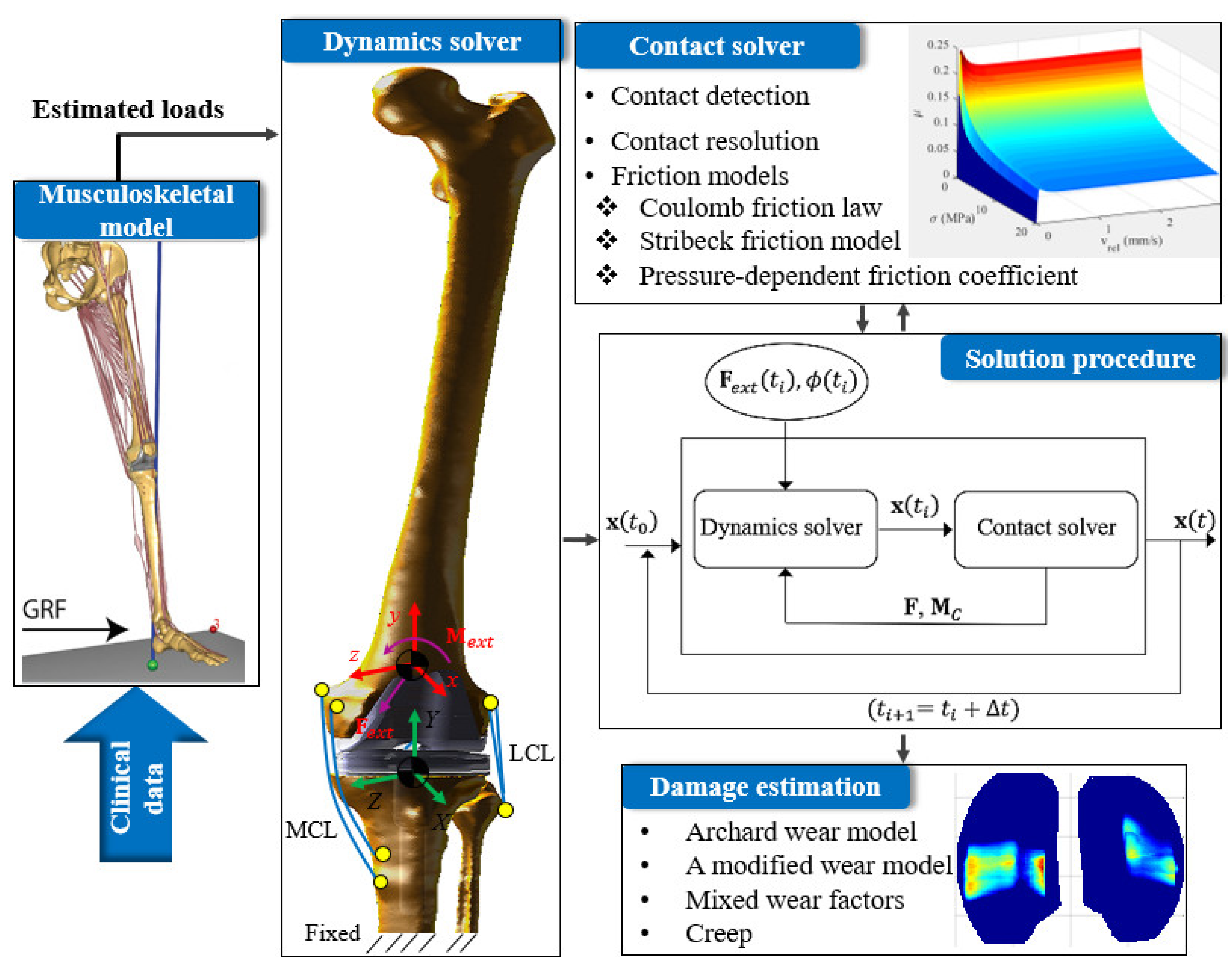
Given the state of the art in this field, the effects of friction on the TKA’s kinematics are yet unclear and remain to be investigated. Therefore, this research work aims at studying friction effects on the joint motion, friction-induced vibration, and the damage of TKAs. Moreover, this research work carries out a comparative study on several phenomenological and empirical friction models integrated into the algorithms accounting for the dynamics of TKA. The computational framework developed in this study also is observable in Figure 1.

2. An Overview on Friction Models

Friction is generally described as the resistance to motion when two surfaces slide against each other. Friction between solid bodies is an extremely complicated physical phenomenon encompassing elastic and plastic deformations of the articulating bodies, chemical reactions, interactions with wear particles, micro-fractures and cracks, excitation of electrons, and the transfer of particles from one body to another. However, it is possible to represent this complex phenomenon using either simple friction laws with a couple of friction parameters or more sophisticated friction models that commonly require determining a larger number of parameters experimentally. One of the first and simplest friction laws is the Coulomb friction law. Coulomb (1736–1806) determined that the frictional force between two bodies pressed together with normal force $\Vert {\mathbf{F}}_n\Vert$ can be calculated by multiplying the normal force and friction coefficient that can be computed empirically [21]. The relation between the applied load and relative velocity has the following mathematical form:

$$F=\left\{\begin{array}{c}-{\mu }_c\Vert F_n\Vert \frac{v_t}{\Vert v_t\Vert } \Vert v_t\Vert >0\\ -F_e:\max \left(\Vert F_e\Vert \right)={\mu }_c\Vert F_n\Vert \Vert v_t\Vert =0\end{array}\right.$$

(1)

where F is the friction force, $v_t$ the tangential sliding speed, ${\mu }_c$ is the Coulomb friction coefficient, and finally $F_e$ is external, tangential force. Using this model to deal with friction in dynamic systems leads to a computational burden due to the discontinuity at zero velocity. The friction force can reach any value between $-{\mu }_c\Vert F_n\Vert$ and ${\mu }_c\Vert F_n\Vert$ due to a sudden alteration in the velocity direction at zero speed. From a physical viewpoint, knowing the external force, imposed on the sliding bodies, can resolve this issue as the friction load is set equal to the externally applied force according to Newton’s first law. Although obtaining the external load is experimentally possible at zero velocity, this is not straightforward to determine in numerical simulations. It is worth noting that the Coulomb friction model only needs one input parameter, i.e., ${\mu }_c$, which is why both academic and industrial communities commonly use this model for systems that do not require very precise quantifications.

Another issue with the Coulomb friction law is that it does not capture the distinction between static and kinematic friction. It is well-known that the external force required to make bodies in contact move from their rest status is higher than that when they are in relative motion. Therefore, the Coulomb friction law is modified by replacing the Coulomb coefficient in Equation (1) with a static friction coefficient, i.e., ${\mu }_s$ (${\mu }_s>{\mu }_c$), which is sometimes called Coulomb friction with stiction.

$$F=\left\{\begin{array}{c}-{\mu }_c\Vert F_n\Vert \frac{v_t}{\Vert v_t\Vert } \Vert v_t\Vert >0\\ -F_e:\max \left(\Vert F_e\Vert \right)={\mu }_s\Vert F_n\Vert \Vert v_t\Vert =0\end{array}\right.$$

(2)

The discontinuity issue at zero velocity is still present in this model, making it hard to detect stick and stick-slip phases of friction between bodies in contact. Moreover, the transition from the stick friction phase to the slip one is not smooth and continuous. To resolve these issues, smooth and continuous Coulomb friction models were developed to prevent the computational burden caused by the force discontinuity by introducing a smooth curve around zero velocity. To this end, several continuous functions have been adopted in the literature, like linear, exponential, and trigonometric function types. One such model is considered here that can be obtained by multiplying the hyperbolic tangent function of velocity to the Coulomb friction model, Equation (1) [53]. This modification, which lets the new model be valid for all $v_t$ from a computational viewpoint, is given by

$$F=-{\mu }_c\Vert F_n\Vert \frac{v_t}{\Vert v_t\Vert }\tanh \left(k\Vert v_t\Vert \right)$$

(3)

in which k is a coefficient that determines how fast the hyperbolic tangent function changes from near 0 to near +1, which can also be represented by $\frac{\Vert v_t\Vert }{v_0}$ where $v_0$ depicts a chosen velocity at which one expects the tanh function to take a value close to its maximum. Another model uses a linear friction−velocity relationship at the proximity of zero velocity to smooth out the discontinuity, which can be expressed as follows [53]:

$$F=-{\mu }_c\Vert F_n\Vert \frac{v_t}{\Vert v_t\Vert }\min \left(k_{sat}\Vert v_t\Vert ,1\right)$$

(4)

in which $k_{sat}$ is the slope of linear function between zero velocity and $1/\Vert v_t\Vert$ to eliminate the difficulty in determining the friction force at zero sliding speed. Obviously, the friction force at zero relative velocity between the interacting bodies is not zero and is equal to the tangential applied force. Hence, the main drawback of the modified Coulomb friction laws explained above is that they assume zero friction at zero relative velocity, which does not make sense from a physics viewpoint.

With the study of lubrication by Rayleigh and Stokes, and the classical paper on theoretical modeling of fluid-film lubrication, which Osborne Reynolds published [54], the following expression for the viscous friction can be written

$$F=-k_v{v}_t$$

(5)

in which $k_{\nu }$ is the viscous coefficient. In full-film contacts, the viscous model can be assumed a good representation of behavior of the system. Moreover, the model can act well enough in other contact conditions provided that the viscous coefficient is tuned. Sometimes a better fit to experimental data can be achieved by assuming a nonlinear term of velocity in Equation (5). As such, Equation (5) can be recast as follows [24]:

$$F=-k_v\Vert v_t\Vert {}^{{\delta }_v}\frac{v_t}{\Vert v_t\Vert }$$

(6)

where the power ${\delta }_v$ depends on the geometry of bodies in relative motion. The viscous friction term can be superimposed on the other friction models such as the Coulomb friction [53], which results in, for example, the following formulation.

$$F=\left\{\begin{array}{c}-{\mu }_c\Vert F_n\Vert \frac{v_t}{\Vert v_t\Vert }-k_v{v}_t \Vert v_t\Vert >0\\ -F_e:\max \left(\Vert F_e\Vert \right)={\mu }_c\Vert F_n\Vert \Vert v_t\Vert =0\end{array}\right.$$

(7)

The Coulomb friction law, and its modified versions, do not explain the negative damping characteristic of friction [11], which was observed by Stribeck as a continuous nonlinear velocity-dependent phenomenon called the Stribeck effect [55].This dependency of friction on the relative sliding velocity was also observed by Panovko and Gubanova [56] and Ibrahim [57] experimentally. The general form of the Stribeck friction model can be written as follows:

$$F=\left\{\begin{array}{c}-\mu \left(\Vert v_t\Vert \right)\Vert F_n\Vert \frac{v_t}{\Vert v_t\Vert } \Vert v_t\Vert >0\\ -F_e:\max \left(\Vert F_e\Vert \right)={\mu }_s\Vert F_n\Vert \Vert v_t\Vert =0\end{array}\right.$$

(8)

where $\mu \left(\Vert v_t\Vert \right)$ is a friction coefficient function for which multiple formulations are available in the literature [58] and one of the common forms of which is given below.

$$\mu (\Vert v_t\Vert )={\mu }_c+\left({\mu }_s-{\mu }_c\right)e^{-{\left(\raisebox{1ex}{$\Vert v_t\Vert $}\!\left/ \!\raisebox{-1ex}{$v_Q$}\right.\right)}^{{\delta }_Q}}$$

(9)

Here, $v_Q$ is the Stribeck velocity, and ${\delta }_Q$ is an exponent that depends on the geometry of the application. It is worth noting that ${\mu }_c$ depicts both the Coulomb friction coefficient and kinetic friction coefficient in this paper while being recognizable according to the context. Friction parameters in Equation (9) can be obtained by performing the friction test for motions with constant velocity. Although the Stribeck friction model is velocity-dependent, this model can be considered a steady friction model. Moreover, the reason for decreasing friction with increasing speed in dry sliding metallic bodies was experimentally investigated and was found to be due to the material softening as a result of high temperatures generated at the contact surfaces [59,60]. Moreover, the friction in a lubricated contact decreases with increasing the relative velocity due to a decrease in the number of surface asperities being in contact until full-film lubrication is obtained. Afterward, the friction can gain a value, and either be constant, increase, or decrease with increasing the sliding speed due to viscous and thermal effects. In the case of an increase in friction when full-film lubrication is built, one can add the viscous friction presented in Equation (5) to the relationship Equation (9) to mimic the intuitive physics. The Stribeck model can provide a good representation of the friction between sliding surfaces. The discontinuity problem of the Coulomb friction model is a problem also observed in the Stribeck model. To cope with this issue, the same procedures taken for the Coulomb friction, like using a hyperbolic tangent function, are applicable here as well. Bengisu and Akay suggested a formulation, Equation (10), which is quite different from that in Equation (9), while resolving the aforementioned discontinuity issue [61].

$$\mu \left(\Vert v_t\Vert \right)=\left\{\begin{array}{c}-\frac{c_s}{v_0^2}{\left(\Vert v_t\Vert -v_0\right)}^2+c_s, \Vert v_t\Vert <v_0 \\ {\mu }_c+\left({\mu }_s-{\mu }_c\right)\exp \left(-\xi \left(\Vert v_t\Vert -v_0\right)\right) \Vert v_t\Vert \ge v_0\end{array}\right.$$

(10)

The first part of the above friction coefficient function uses a near-zero continuous curve to avoid divergence of the numerical model. The second term is the Stribeck friction relation. In addition, $\xi >0$ is the negative slope of the sliding state [62]. After the friction coefficient starts from zero, it increases to peak friction, which Bengisu and Akay [61] referred to as the static friction coefficient, ${\mu }_s$. The friction coefficient then reduces with increasing tangential velocity until the friction finally reaches a steady state, i.e., ${\mu }_c$.

As was discussed previously, the aforementioned models are not efficient to determine friction magnitude when the velocity is zero nor to manage the stiction phenomenon. Karnopp introduced a concept of the dead-velocity band of the zero proximity, i.e., $\Vert v_t\Vert <v_D$, to cope with the difficulties encountered to detect zero velocity and prevent switching between multi-state relationships to transit between stick, stick-slip and pure slip phases of the friction [63]. Within the abovementioned velocity interval, the speed is assumed to be null. The friction phase also is stiction, where the friction force can be equal to either tangential external force or static friction. For the velocities outside of that dead band, the friction force can get the form of Coulomb friction, Stibeck friction, and so forth. The following equation can express this idea.

$$F=\left\{\begin{array}{c}-\min \left(\Vert F_e\Vert , \Vert F_s\Vert \right)\frac{F_e}{\Vert F_e\Vert } \Vert v_t\Vert <v_D\\ \mathbf{F}\left(v_t\right), \Vert v_t\Vert \ge v_D\end{array}\right.$$

(11)

However, the concept Karnopp used to introduce this friction model does not comply with friction physics. Moreover, this model requires the external load as an input, which is often not available explicitly and is an internal state of the dynamical system.

In addition to the phenomenological friction models, there are empirical friction models proposed for UHMWPE in the literature. Wang et al. [26] reported the following formula derived from experimental data, showing a significant correlation to the contact stress. However, the Coulomb friction model and its modified versions cannot address changes in friction coefficient due to contact stress:

$$\mu =0.18 {\sigma }^{-0.33}$$

(12)

in which $\mu$ stands for the friction coefficient and $\sigma$ is the contact stress with a unit of MPa. Furthermore, another empirical formulation was suggested by Saikko to relate the friction coefficient to the contact stress as follows [27]:

$$\mu =0.32{\left(\frac{\sigma }{{\sigma }_{ref}}\right)}^{-0.68}$$

(13)

where ${\sigma }_{ref}$ is a reference pressure (1.1 MPa). The above relationship is correct for $\sigma \ge 1.1 \mathrm{MPa}$ and below this pressure, the coefficient of friction increases with increasing the contact pressure. Recently, several empirical friction models for tibiofemoral joints were developed by a research group in Mexico [28,29]. Montes-Seguedo et al. [30] proposed a power-law model from which the friction coefficient can be estimated in both mixed lubrication regime and full-film lubrication regime as a function of the maximum pressure (${\sigma }_{max}$), entrainment velocity ($v_m$) in mm/s, and sliding-to-rolling ratio (SRR), which is written as follows.

$$\mu =0.54·{\sigma }_{max}^{-0.58}·SR{R}^{-0.1}·{\left|v_m\right|}^{-0.1}$$

(14)

Models discussed above are not able to capture dynamic friction characteristics such as pre-sliding and frictional lag. Dynamic friction models such as the Dahl approach and LuGre model can address such phenomena. The discussion associated with the dynamic friction models stands out of the scope of the present study. Interested readers are referred to the following references [24,64,65,66,67] for further information

3. Contact Solver: Tangential Friction and Normal Contact Forces

As was discussed before, when two surfaces enter into a contact phase and tend to slide against each other, friction develops and acts as a resistance to the relative motion. In this study, the friction forces are taken into account employing several friction models, listed in

Table 1. Friction models used in the dynamic modeling of TKA.

Main Friction Model Structure	Friction Coefficient	Model No.
A. Modified Coulomb friction model: $\mu \left(\Vert u_t^{k,j}\Vert ,{\sigma }_{k,j}\right)=\left\{\begin{array}{c}{\mu }_c \Vert u_t^{k,j}\Vert \ge v_0\\ \frac{\Vert u_t^{k,j}\Vert }{v_0}{\mu }_c \Vert u_t^{k,j}\Vert <v_0\end{array}\right.$	${\mu }_c=constant$	A1
	${\mu }_c={\mu }_c\left({\sigma }_{k,j}\right)=$ $\left\{\begin{array}{c}0.18\times {\sigma }_{k,j}^{-0.33} {\sigma }_{k,j}\ge 0.37 \mathrm{MPa}\\ 0.25 {\sigma }_{k,j}<0.37 \mathrm{MPa}\end{array}\right.$	A2
	${\mu }_c={\mu }_c\left({\sigma }_{k,j}\right)=$ $\left\{\begin{array}{c}0.32{\left(\frac{{\sigma }_{k,j}}{{\sigma }_{ref}}\right)}^{-0.68} {\sigma }_{k,j}\ge 1.1\\ 0.32-0.0579{\left({\sigma }_{k,j}-1.1\right)}^2 {\sigma }_{k,j}<1.1\end{array}\right.$	A3
B. Stribeck friction model: $\mu \left(\Vert u_t^{k,j}\Vert ,{\sigma }_{k,j}\right)=$ $\left\{\begin{array}{c}-\frac{{\mu }_s}{v_0^2}{\left(\Vert u_t^{k,j}\Vert -v_0\right)}^2+{\mu }_s, \Vert u_t^{k,j}\Vert <v_0 \\ {\mu }_c+\left({\mu }_s-{\mu }_c\right)e^{-\xi \left(\Vert u_t^{k,j}\Vert -v_0\right)} \Vert u_t^{k,j}\Vert \ge v_0\end{array}\right.$	${\mu }_c=constant$ and ${\mu }_s=constant$	B1
	${\mu }_c={\mu }_c\left({\sigma }_{k,j}\right)=$ $\left\{\begin{array}{c}0.18\times {\sigma }_{k,j}^{-0.33} {\sigma }_{k,j}\ge 0.37 \mathrm{MPa}\\ 0.25 {\sigma }_{k,j}<0.37 \mathrm{MPa}\end{array}\right.$   ${\mu }_s={\mu }_s\left({\sigma }_{k,j}\right)=\chi \times {\mu }_c\left({\sigma }_{k,j}\right)$	B2
	${\mu }_c={\mu }_c\left({\sigma }_{k,j}\right)=$ $\left\{\begin{array}{c}0.32\times {\left(\frac{{\sigma }_{k,j}}{{\sigma }_{ref}}\right)}^{-0.68} {\sigma }_{k,j}\ge 1.1\\ 0.32-0.0579{\left({\sigma }_{k,j}-1.1\right)}^2 {\sigma }_{k,j}<1.1\end{array}\right.$   ${\mu }_s={\mu }_s\left({\sigma }_{k,j}\right)=\chi \times {\mu }_c\left({\sigma }_{k,j}\right)$	B3
C. Montes-Seguedo et al.’s model $\mu =0.54·{\sigma }_{max}^{-0.58}·SR{R}^{-0.1}·{\left|v_m\right|}^{-0.1}$	$SRR=\left|\frac{v_r}{v_m}\right|$; $v_r=v_F-v_T$; $v_m=\frac{(v_F+v_T)}{2}$;	C1

, that are: (A₁) a modified Coulomb friction model with a constant friction coefficient; (A₂) a modified Coulomb friction model with a pressure-dependent friction coefficient extracted from Wang et al.’s formulation; (A₃) a modified Coulomb friction model with a pressure-dependent friction coefficient extracted from Saikko’s formulation; (B₁) a Stribeck friction approach with constant friction coefficients; (B₂) a Stribeck friction approach with pressure-dependent friction coefficients extracted from Wang et al.’s formulation; (B₃) a Stribeck friction approach with pressure-dependent friction coefficients extracted from Saikko’s formulation; and (C₁) Montes-Seguedo et al.’s empirical friction model. The tangential friction force at a node of the femoral part, e.g., $Q_F^{k,j}$, is computed using the following formulation:

$$F^{k,j}=-\mu \left(\Vert u_t^{k,j}\Vert ,{\sigma }_{k,j}\right)\Vert F_n^{k,j}\Vert \frac{u_t^{k,j}}{\Vert u_t^{k,j}\Vert }$$

(15)

where $u_t^{k,j}$ is the tangential relative velocity of the node $Q_F^{k,j}$ in contact as the tibial insert is assumed stationary, and $\mu \left(\Vert u_t^{k,j}\Vert ,{\sigma }_{k,j}\right)$ is the friction coefficient at the contacting node, which can be considered as a function of either relative velocity or contact pressure and can be substituted from each of the modified Coulomb friction and Stribeck friction models, outlined in Table 1. Moreover, static and dynamic friction coefficients can be dependent upon the contact stress based on empirical models reported by Wang et al. [26] and Saikko [27]. Eventually, seven case scenarios are defined in Table 1, each of which is considered in this study to study kinematics and tribology of TKAs.

In Table 1, $\chi$ is a constant value that takes a value greater than one. Moreover, the pressure-dependent friction coefficient is used in the models A₂ and B₂, illustrated in Figure 2, to show the difference between such models. As can be seen, the friction coefficient is a function of both relative velocity and pressure when model B₂ is employed, while it varies merely with contact pressure in model A₂. It is worth adding that both models use the pressure-dependent friction relationship Wang et al., proposed in [26]. However, such a relationship is integrated into the Coulomb friction formula for model A₂ and the Stribeck one for model B₂. It is worth noting that the empirical model Wang et al. [26] suggested does not address the friction coefficient once the contact stress approaches zero. Therefore, the strategy considered here is to prevent the friction coefficient to exceed the value 0.25 that corresponds to the contact stress of 0.37 MPa. In addition, the models A₃ and B₃ are written based on the relationship recommended by Saikko. His empirical mathematical formulation is valid for the contact stress equal or greater than 1.1 MPa. According to the plot that shows the relationship between the contact stress and friction coefficient in his paper, it can be concluded that the friction coefficient decreases once the contact stress diminishes below 1.1 MPa until it gains an average value of 0.25 once the contact stress reaches zero value. Therefore, a quadratic function is fitted to the data while outliers are removed to address the value of friction once the contact stress gains a value less than 1.1 MPa. The model C₁ is the one developed by Montes-Seguedo et al. [30], in which $v_F$ is the velocity of the femoral part at the contact point, which is calculated according to the radius of the functional flexion-extension axis, multiplied by the respective angular velocity and $v_T,$ the speed of the tibial insert at the tibial plateau surface. The latter is computed as the summation of the anterior-posterior linear velocity and the multiplication of the radial distance from the tibial axis to the bottom of the tibial plateau and the internal-external angular velocity. For further information on how to determine these velocity terms, the reader is referred to the reference [28].

At this stage, a short description of the joint kinematic is presented to determine the velocity of master nodes, including their tangential speed. The relative velocity of a master node like $Q_F^{k,j}$ with respect to its corresponding slave node $Q_T^{k,j}$ locating on body 2, i.e., the tibial insert, can be determined as follows:

$$U^{k,j}={\dot{X}}^{t_n}+{\Omega }_F\times \left(Q_F^{k,j}-X^{t_n}\right)$$

(16)

$$u_n^{k,j}=\left(U^{k,j}·{}^{tn}n_F^{k,j}\right){}^{tn}n_F^{k,j}$$

(17)

$$u_t^{k,j}=U^{k,j}-u_n^{k,j}$$

(18)

where $U^{k,j}$ is the velocity vector of the point $Q_F^{k,j}$ with respect to $Q_T^{k,j}$, ${\dot{X}}^{t_n}$ and ${\Omega }_F$ depict the translational velocity of the local coordinate system and the angular velocity of body 1, respectively, $Q_F^{k,j}$ depicts the coordinate vector of the point $Q_F^{k,j},$ and $X^{t_n}$ is the location of the origin of the local coordinate of body 1, i.e., the femoral body, at time t_n$. {}^{tn}n_F^{k,j}$ is the vector normal to the femoral body at the point $Q_F^{k,j}$ at time t_n. and $u_n^{k,j}$ and $u_t^{k,j}$ also are the normal and tangential relative velocities of the point $Q_F^{k,j}$. As body 2 is assumed stationary, the components of the angular velocity vector resolved in the fixed basis could be evaluated based on Euler angles as follows [68]:

$${\Omega }_F=H_{z-x-y}\left\{\begin{array}{c}\dot{\varphi }\\ \dot{\theta }\\ \dot{\psi }\end{array}\right\}$$

(19)

where

$$H_{z-x-y}=\left[\begin{array}{ccc}0\hfill & \cos \varphi & -\sin \varphi \cos \theta \\ 0\hfill & \sin \varphi & \cos \varphi \cos \theta \\ 1\hfill & 0& \sin \theta \end{array}\right]$$

(20)

in which $\left\{\varphi , \theta ,\psi \right\}$ are Euler angles and $\left\{\dot{\varphi }, \dot{\theta },\dot{\psi }\right\}$ depict their time derivatives.

Eventually, the friction force at each element on the femoral components is evaluated knowing the tangential sliding velocities, Equation (18) at all element nodes, the normal load applied to the element, and contact pressure, which are addressed later in this paper. Finally, the resultant friction force tangentially applied to the femoral component can be obtained from the following integration that is performed over the contact area:

$$F_{\mu }={{\displaystyle \iint }}_{\mathsf{\Omega }}F dA={\displaystyle \sum }_k{\displaystyle \sum }_j{F}^{k,j}d{A}^{k,j}$$

(21)

where $\mathsf{\Omega }$ depicts the contact area, $F^{k,j}$ is friction force at each element and $d{A}^{k,j}$ depicts the size of element area.

The present study implements a concept proposed in [69] to evaluate contact stresses, but it is impossible to derive a closed-form mathematical formulation for the contact problem at hand. Askari obtained nonlinear and promising contact models while resolving the discontinuity issue with the Kelvin-Voigt model at both the beginning and end of the contact process [69]. To this end, he simulated the contact by using a set of independent springs and dashpots, which represent the stiffness and viscous damping of the contact between articulating bodies, respectively. Readers interested are referred to the reference [69,70,71,72] and references therein for further information about the model employed in this study. Such a contact model does not put any kinematic constraints on the dynamical system. It is well-known that the Kelvin-Voigt model suffers from a discontinuity at both the beginning and end of the contact process due to the form of the damping term in its formulation [73,74]. 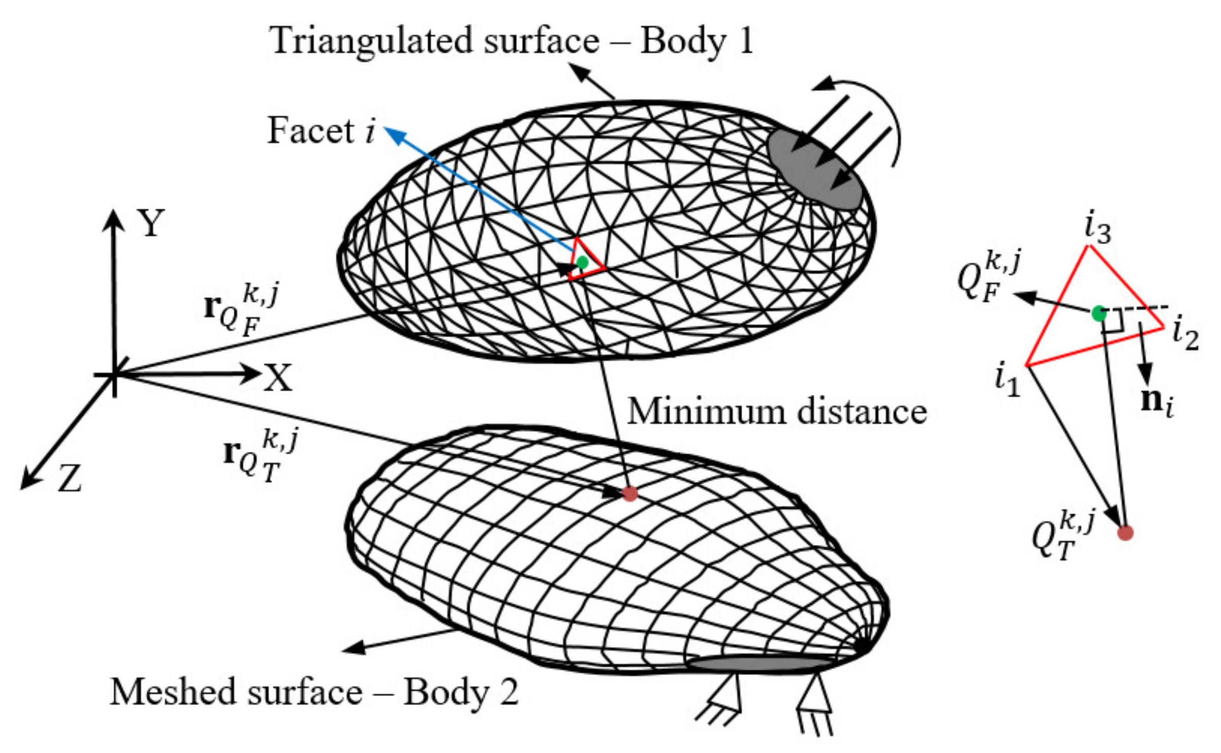The concept proposed in the reference [69] showed that simulating a soft contact using a set of independent Kelvin-Voigt elements spread all over the contact surfaces instead of just one spring-damper element as is used in the Kelvin-Voigt contact model can resolve the above discontinuity. The penetration depth at each node on the polyethylene surface, $D_{k,j}$, is known from the minimum distance technique discussed later in the present paper (see Section 5.3). Its time derivative ${\dot{D}}_{k,j}$ is also obtained from the normal velocity term given in Equation (17). Therefore, the normal contact pressure, i.e., ${\sigma }^{k,j}$, at any node of $Q_T^{k,j}$ can be determined based on the following Kelvin−Voigt contact relationship:

$${\sigma }^{k,j}=-K{D}_{k,j}-K\tau {\dot{D}}_{k,j}$$

(22)

in which $K$ is the contact stiffness and $\tau$ the relaxation time, $K$ is obtained from $K=\mathsf{\Lambda }/\mathsf{\Xi }$ where $\mathsf{\Lambda }=\left(1-\upsilon \right)E/\left[\left(1+\upsilon \right)\left(1-2\upsilon \right)\right]$ and $\mathsf{\Xi }$ is the tibia thickness [40], E and $\upsilon$ are Young’s modulus and Poisson’s ratio of the polyethylene that are, respectively, 463 MPa and 0.46 as are reported in [75,76,77]. Such a contact model belongs to the category of the penalty non-adhesive contact approaches and penalizes the indentation of the master body into the slave one. As independent Kelvin−Voigt elements are spread all over the contact area, the normal contact force applied to the femoral components should be computed by performing the following integration over the contact area:

$$F_{cont}={{\displaystyle \iint }}_A\sigma n_F dA$$

(23)

where $n_F$ is the normal unit vector of an element with the area $dA$ on the femur-bearing surface. It is worth noting that the following criterion is used to assess whether a node is in contact or not.

$$\left\{\begin{array}{c}{D}_{i,j}>0 no contact \\ D_{i,j}\le 0 contact \end{array}\right.$$

(24)

The resultant contact area can also be obtained according to the summation of the area associated with all elements engaged in contact area having nodes with non-zero contact pressure.

4. Patient-Specific Musculoskeletal Modeling

To estimate patient-specific TKA knee joint loads, an already validated, patient-specific musculoskeletal model is applied [35]. This model is based on data for one male subject (age: 86, height: 1.80 m and mass: 75 kg) with an instrumented, posterior cruciate-retaining TKA prosthesis from the 5th Grand Challenge Competition to Predict In Vivo Knee Loads [78,79,80]. For more details of the implant shape and design, the reader is referred to the Grand Challenge knee dataset [78]. Among others, the dataset contains pre- and post-operative Computed Tomography (CT) scans, trajectories of skin markers and ground reactions during standing reference trials and dynamic movement trials, including gait at a self-selected speed as well as measurements from the instrumented knee prosthesis. Additionally, Stereolithography (STL) 3D geometries of the femoral component, tibial tray and insert, patellar button, and segmentation of the post-operative CTs of the partial pelvis, femur, patella, tibia, fibula, partial talus and partial calcaneus are also included in the dataset [81]. For the dynamic analysis, the one gait trial of level walking at self-selected speed (PS_ngait_og_ss1) is utilized [78]. The musculoskeletal model is developed using the AnyBody Modeling System (AMS) v. 7.1 (AnyBody Technology A/S, Aalborg, Denmark) and based on the human model from the AnyBody Managed Model Repository (AMMR) v. 1.6. From this model, we extract all the knee flexion-extension angles as well as all loads associated with muscle, hip joint, gravitational, inertial, etc., which are imposed on the femur. The tibiofemoral joint reaction forces and knee ligament loads are included in the joint model described below and, therefore, are not part of that model’s boundary conditions.

5. Dynamics Solver

In this section, a forward dynamic model of the tibiofemoral joint is presented. We focus on an assembly consisting of the tibia and femur as the tibiofemoral joint’s components along with its ligaments to develop the forward dynamic model to which damage prediction approaches are later added. In the following, the development process of such a model illustrated in Figure 1 is described in detail. A forward dynamics model is first derived, which requires the evaluation of contact stresses and ligament forces and moments before being solved. To determine contact stresses, triangulated surfaces of bearing components are smoothed and contact detection is performed.

5.1. Dynamics Modeling

The governing equations of the system motion are derived based on the free body diagram of the tibiofemoral joint represented in the second right-hand panel of Figure 1. The resulting forces and moments applied to the femoral bone due to the existence of all surrounding soft tissues such as muscles and hip-joint reactions are computed by means of musculoskeletal modeling. Such loadings and moments are moved to the origin of the femur coordinate system and written in the global coordinate system, illustrated in the second right-hand panel of Figure 1, as F_ext and M_ext. The loads and moments owing to the contact, friction, and ligaments are also determined and summed up to those external ones. The governing equations of the translational motion of the femoral component, therefore, can be formulated using Newton’s second law of motion as follows [69,82]:

$$M\ddot{X}=F_T,F_T=F_{ext}+F_{cont}+F_{\mu }+F_{lig}$$

(25)

in which the mass of the femoral bone is designated by M. The translational acceleration vector of the femur is also depicted by $\ddot{X}$. Furthermore, $F_T$ stands for the vectorial summation of forces imposed on the bone, which is mathematically formulated in Equation (25). In this equation, the external forces are depoicted by $F_{ext}$, resultant contact forces $F_{cont}$, friction force $F_{\mu }$, and finally ligaments loads are designated by $F_{lig}$. In this solution setup, three coordinate systems are defined, one of which is the global coordinate system (XYZ) attached to the underneath of the tibial insert and on the top of the tibial tray. It is worth mentioning that the tibia is considered stationary, while the femur has six degrees of freedom to translate and rotate. One degree of freedom of this dynamic system is, later, constrained while knowing the flexion-extension angle of the knee joint over a level walking gait. The other coordinate system is a local system (xyz) attached to the STL center of the femoral component, rotating and translating with the femur. However, the third coordinate system, $\xi \eta \zeta$, is considered with the same origin as the femoral coordinate system, although it does not rotate with the femur and it has bases aligned with those of the global coordinate system. The angular-momentum equation can now be written in the body coordinate system of the femur, which governs the rotational motion of the femur as follows [69]:

$$M_C^{*}=I^{C*}{\dot{\omega }}^{*}+{\tilde{\omega }}^{*}{I}^{C*}{\omega }^{*}$$

(26)

where $M_C^{*}$ is the summation of not only external moments but also those resulted from the contact, friction and ligaments, which are computed with respect to the body coordinate system of the femoral part (xyz). Compared to the computation of moments in the coordinate system xyz, it is much easier to obtain moments in the third coordinate system discussed above. The summation of moments in the third coordinate system is designated by $M_C$ and is related to $M_C^{*}$ by the following relationship:

$$M_C^{*}=R^T{M}_C$$

(27)

in which $R^T$ is the transpose of the rotation tensor of the femur, $I^{C*}$ and ${\omega }^{*}$ appeared in Equation (26) and stand for the tensor of inertia and the angular velocity vector of the femoral component in the body coordinate system, respectively. In the dynamic model developed in this study, the rotation tensor is defined based on the Euler angles of the z-x-y sequence, given by the array of Euler angles $q^T=\left\{\varphi , \theta ,\psi \right\}$ to characterize the rotation of the femur as well as the location of nodes on the femoral-bearing surface. The respective rotation tensor can be cast by:

$$R\equiv R_{z-x-y}=\left[\begin{array}{ccc}\cos \varphi \cos \psi -\sin \varphi \sin \theta \sin \psi & -\sin \varphi \cos \theta & \cos \varphi \sin \psi +\sin \varphi \sin \theta \cos \psi \\ \sin \varphi \cos \psi +\cos \varphi \sin \theta \sin \psi & \cos \varphi \cos \theta & \sin \varphi \sin \psi -\cos \varphi \sin \theta \cos \psi \\ -\cos \theta \sin \psi & \sin \theta & \cos \theta \cos \psi \end{array}\right]$$

(28)

where the flexion-extension angle, which is the amount of the planar rotation of the femur around the axis z, is named by $\varphi$. From the time derivatives of Euler angles, the angular velocity vector in the body coordinate system can be given by:

$${\omega }^{*}=H_{z-x-y}^{*}\left\{\begin{array}{c}\dot{\varphi }\\ \dot{\theta }\\ \dot{\psi }\end{array}\right\}$$

(29)

where

$$H_{z-x-y}^{*}=\left[\begin{array}{ccc}-\cos \theta \sin \psi & \cos \psi & 0\\ \sin \theta & 0& 1\\ \cos \theta \cos \psi & \sin \psi & 0\end{array}\right]$$

(30)

The tangent operator $H_{z-x-y}^{*}$ is tangent to the rotation manifold. There is a possibility to simplify Equation (26) while setting the body coordinate system such that it coincides with the principal axes of the mass moment of inertia tensor, i.e., $I^{C*}$. Hence, the moment of inertia tensor is reduced to a diagonal form, and the governing equations turns to the so-called Euler’s equations for the angular motion of the dynamic system as follows.

$$\begin{array}{c}{M}_{Cx}^{*}=I_{xx}^{C*}{\dot{\omega }}_x^{*}-\left(I_{yy}^{C*}-I_{zz}^{C*}\right){\omega }_y^{*}{\omega }_z^{*}\\ M_{Cy}^{*}=I_{yy}^{C*}{\dot{\omega }}_y^{*}-\left(I_{zz}^{C*}-I_{xx}^{C*}\right){\omega }_x^{*}{\omega }_z^{*}\\ M_{Cz}^{*}=I_{zz}^{C*}{\dot{\omega }}_z^{*}-\left(I_{xx}^{C*}-I_{yy}^{C*}\right){\omega }_y^{*}{\omega }_x^{*}\end{array}$$

(31)

Characterizing of the femoral bone along with surrounding tissues of the male subject, the femoral mass, i.e., M, is 7.5 kg and its moment of inertia tensor is obtained as (0.4516 0 0; 0 0.0213 0; 0 0 0.4516) [35,78]. The adaptive Runge−Kutta−Fehlberg approach is employed to integrate Equations (25) and (31) over time of interest [83]. A maximum error is set and the error magnitude at each time step of the numerical simulation is assessed while comparing outcomes from the above method of different orders 4 and 5. Once the error acquired is greater than the set maximum error, the time step is halved and the computational process is done again until the accuracy and stability of outcomes become guaranteed. The present study also considers a minimum value of the integration time-step size 5 × 10⁻⁵s along with an integration tolerance 5 × 10⁻⁶ [84].

5.2. Ligament Modeling: Ligament Forces and Moments

In this study, ligament forces are modeled using an asymmetric nonlinear elastic model. The force, $f\left(\epsilon \right)$, each ligament, i.e., PCL, LCL, and MCL, imposed on the femur can be evaluated from the following formula, which also includes a slack region [85].

$$f\left(\epsilon \right)=\left\{\begin{array}{cc}\frac{k_l{\epsilon }^2}{4{\epsilon }_1}& 0\le \epsilon \le 2{\epsilon }_1\\ k_l\left(\epsilon -{\epsilon }_1\right)& \epsilon >2{\epsilon }_1\\ 0& \epsilon <0\end{array}\right.$$

(32)

Here, $k_l$ is the ligament stiffness and $\epsilon$ depicts the strain while ${\epsilon }_1$ is a constant with value of 0.03, which is associated with the transition phase between linear and nonlinear regions of the force-strain curve. In order to determine the ligament strain, the slack length, l₀, is obtained as below:

$$l_0=\frac{l_r}{{\epsilon }_r+1}$$

(33)

where ${\epsilon }_r$ is the reference strain and l_r stands for the bundle length estimated when the leg is fully extended. Finally, the strain, $\epsilon$, at any time is computed from the following equation:

$$\epsilon =\frac{l-l_0}{l_0}$$

(34)

in which l is the instantaneous bundle length of the ligament, which is determined according to the motion of the femur over the walking activity. Wrapping surfaces are also employed to prevent ligaments from penetrating the bones and the implant. Stiffness and reference strain assigned to each ligament bundle are extracted from [35,86], which are adapted from the literature [85]. To compute ligament forces, the insertion points of every single ligament are assigned before the numerical simulation starts. Since attachment sites could not be determined from the dataset, they are estimated according to descriptions found in the literature [35,87,88]. The motion of the femoral component at each time step is acquired using motion equations, given by Equations (25) and (31), and the rotation tensor, Equation (28). Therefore, we can now determine the current locations of insertion points in the global coordinate system. Moreover, each ligament is discretized into several elements to calculate their time-dependent length according to the femoral motion. The magnitude of each force is, in turn, obtained while solving Equations (32)–(34) and the corresponding vector direction is considered to be along the ligament tangent at its insertion point. The resulting ligament force and moment imposed on the femur are computed by

$$F_{lig}=F_{LCL}+F_{PCL}+F_{MCL},\hspace{1em}{M}_{lig}=M_{LCL}+M_{PCL}+M_{MCL}$$

(35)

5.3. Contact Detection

STL 3D geometry files of the knee components are available from the Grand Challenge knee dataset [78]. After removing facets and respective vertices that are not likely to get into contact, the triangulated surfaces of the contacting pair are smoothed using a Laplacian smoothing technique. As the tibial insert is assumed stationary, its bearing surface is constructed using the Non-Uniform Rational B-Spline (NURBS) surface methodology [40,89,90] and, in turn, is meshed using a uniform mesh size in the first place. A bounding box scheme is applied to the meshed surface of the tibia to reduce the computational time of searching spatial contact. All boxes, susceptible to the contact incident while deemed based on a one-by-one surface function-based scheme, are retained. In the next step, each box becomes open and each node inside is assessed for whether it is in contact with the femoral component or not using the minimum distance technique described as follows. The minimum distance of a node such as $Q_T^{k,j}$ on the slave-bearing surface with respect to the femoral body can be obtained as is described as follows. A facet with number i, belonging to the triangulated surface of the body 1, is considered and a vector is drawn from the first vertex of the facet i, i.e., $i_1$, to the node of interest (see Figure 3). This vector is, in turn, projected on the vector normal to the facet under consideration, which is designated by $\overrightarrow{i_1{Q}_T^{k,j}}$ and its magnitude is equal to its ${\ell }_2$ norm $\Vert \overrightarrow{i_1{Q}_T^{k,j}}{\Vert }_2$. Then, the projection of the node $Q_T^{k,j}$ on the plane of the facet i is obtained and called $Q_F^{k.j}$. By this time, the question is whether that projected point, i.e., $Q_F^{k.j}$, places inside the domain of the facet i. To check it out, the summation of angles between each two of the three following vectors, $\overrightarrow{Q_F^{k,j}{i}_1}$, $\overrightarrow{Q_F^{k,j}{i}_2}$, and $\overrightarrow{Q_F^{k,j}{i}_3}$, as illustrated in Figure 3, is acquired. The ${\ell }_2$ norm of each of those three vectors is also computed. If either of the following cases takes place, it is confirmed that the point $Q_F^{k,j}$ corresponds to the likely contact point on the master body and the minimum distance of the node $Q_T^{k,j}$ with respect to the femoral surface is then acquired, i.e., $\Vert \overrightarrow{Q_T^{k,j}{Q}_F^{k,j}}{\Vert }_2$, and stored as the penetration depth $D_{k,j}$ in the penetration matrix D: (i) the summation of the above three angles is equal to $2\pi$; (ii) the ${\ell }_2$ norm of one of those vectors is zero, so $Q_F^{k,j}$ and the respective vertex are coincident.

6. Damage Formulation

Now that the dynamic model is ready to be used, the tribology of TKA is formulated to predict wear. Archard wear model is commonly used by the tribology community to describe adhesive and abrasive wear mechanisms, although it is often adopted for a wide range of applications as a result of its efficiency and simplicity [36]. Employing Archard wear law, the linear wear rate can be computed using the following expression [91,92]:

$$\frac{dh}{ds}=k_w\sigma$$

(36)

in which the wear depth and sliding distance are presented by h and s, respectively. The parameter k_W stands for the wear factor that has the following unit mm³N⁻¹m⁻¹. Although the wear factor has been considered constant by several research studies, Equation (37), Kang et al., observed from experimental data that the wear factor is dependent on the contact pressure and cross-shear ratio. Therefore, they suggested a new formulation for the wear factor that varies with not only the cross-shear ratio, $\Im$, but also the contact pressure. They proposed a relationship to compute the wear factor of the UHMWPE tibial insert [93] accounting for such dependencies given in Equation (38) in which the average contact stress, i.e., $\overline{\sigma }$, for a given element is computed by averaging contact pressure over one gait cycle, and the definition of the cross-shear ratio and the procedure to compute it is well-described in [93].The described wear techniques listed in

Table 2. Wear factors suggested to be used in Archard wear model for UHMWPE tibial insert.

Wear Model	Formulations
Model i	$\frac{dh}{ds}=k_w\sigma$; $k_w=cons$	(37)
Model ii	$\frac{dh}{ds}=k_w\sigma$; $k_w\left(\Im ,\overline{\sigma }\right)=\exp \left[-13.1+0.19\ln \left(\Im \right)-0.29\overline{\sigma }\right]$	(38)
Model iii	$W=AC$; $C={\left(a+b\times CS\right)}^{-1/c}$	(39)

are used in this study to estimate wear in total knee arthroplasties

Wear factor given in Equation (38) is dependent on the contact pressure and is not easily implemented into computational wear modeling. Abdelgaied et al. [77] developed a wear model based on the idea that volumetric wear (W) is proportional to the contact area (A) and sliding distance (S) and a non-dimensional wear coefficient (C) determined experimentally to complete the wear formulation, Equation (39). The cross-shear ratio is CS, and parameters a, b and c are constant and determined from the experimental measurements of a multi-directional pin-on-disk wear test [77] as a = 8.5173e-65, b = 9.3652e-60, and c = −6.7454.

6.1. Cross-Shear Ratio

Under the sliding motion of a metallic part on ultra-high molecular weight polyethylene, the polymeric chains align in the direction of the maximum frictional work according to the experimental findings [15,94], which is the so-called principal molecular orientation (PMO) [12,15]. The cross-shear ratio can be quantified as the quotient of the frictional work done perpendicular to the PMO direction ($W_{\mathrm{cs}}^f$) to the total frictional work ($W_{\mathrm{T}}^f$) as is formulated below [95,96,97].

$$\Im =\frac{W_{\mathrm{cs}}^f}{W_{\mathrm{T}}^f}$$

(40)

The frictional work can be calculated based on $W^f=\sum _{i=1}^n{F}_{\mu }\left(v_t,\sigma , t_i\right)·\Delta s\left(t_i\right)$ where $\Delta s\left(t_i\right)$ is the incremental sliding distance that can be computed by $\Delta s\left(t_i\right)=u_t^{k,j}\left(t_i\right)\Delta t_i$ at each element. The direction (${\phi }_f$) of incremental motion along the contact point trajectory is calculated to determine the vector of the incremental sliding distance, $\Delta s \left(t_i\right)$. Moreover, considering a test PMO direction (axis) with an angle $\phi$, frictional force and incremental sliding distance components parallel to and perpendicular to that axis can be calculated for each increment [12,95,96]. Assuming that the friction coefficient does not vary during a cycle, the cross-shear can be formulated as follows.

$$\Im =\frac{{\sum }_{i=1}^n\Vert F_{\mu }\left(v_t,\sigma , t_i\right)\Vert \Vert \Delta s\left(t_i\right)\Vert {\sin }^2\left({\phi }_f\left(t_i\right)-\phi \right)}{\sum F_{\mu }\left(v_t,\sigma , t_i\right)·\Delta s\left(t_i\right)}$$

(41)

The dynamic model developed in the previous sections obtains the sliding distance and contact force with time, which allows calculating Equation (41) for each angle $\phi$, from 0 to π, until the principal molecular orientation, ${\phi }_{PMO}$, is reached where the cross-shear ratio is minimized.

6.2. Creep Estimation

In addition to the wear phenomenon, creep deformation contributes to the surface damage of the UHMWPE tibial insert due to the viscoelasticity of UHMWPE, where deformation under a constant load varies with time. Performing experimental creep tests, Lee and Pienkowski [16] presented a nice formulation to compute the creep deformation, which is a function of both pressure and a logarithmic timescale as follows [92]:

$${\delta }_{Creep}^{\left(k,j\right)}=\left[3.491\times {10}^{-3}+7.996\times {10}^{-4}\left(log\left(N{\displaystyle \sum }_{i=1}^n{\Delta }^{\left(k,j\right)}{t}_c\left(i\right)\right)-4\right)\right]\frac{{\sum }_{i=1}^n{P}^{\left(k,j\right)}\left(t_i\right){\Delta }^{\left(k,j\right)}{t}_c\left(i\right)}{{\sum }_{i=1}^n{\Delta }^{\left(k,j\right)}{t}_c\left(i\right)}{\mathsf{\Gamma }}^{\left(k,j\right)}$$

(42)

where ${\delta }_{Creep}^{\left(k,j\right)}$ is the linear damage at an element (k, j) due to creep, N is the total number of cycles in service, ${\mathsf{\Gamma }}^{\left(k,j\right)}$ is the thickness of element (k, j) of the acetabular cup and ${\Delta }^{\left(k,j\right)}{t}_c\left(i\right)$ associated with an element (k, j) of the cup surface is non-zero just when the corresponding i is in the set of time values where the contact stress is non-zero. The unit of time and pressure are minute and MPa, respectively, according to Lee and Pienkowski experiment.

7. Convergence and Mesh Analysis

To guarantee the accuracy and convergence of dynamics and contact simulations, a mesh density analysis is performed [98]. Three different element sizes to discretize the domain of the bearing components projected on the XZ plane are considered, i.e., 0.2, 0.4, and 0.6 mm. Multiple system parameters that can be influenced by the mesh size are used to assess the mesh density, such as contact forces and moments on both medial and lateral condyles, and maximum contact pressures on both condyles. According to the outcomes we obtained at different percentages of the gait cycle, it has been concluded that mesh sizes 0.2 and 0.4 produce accurate results. The latter is used in this study to perform the computational analysis. The respective outcomes corresponding to two pressure peaks in a gait walking cycle, for example, are listed in

Table 3. Mesh density analysis at two peaks of a normal walking gait cycle.

Element Size (mm) and Number	Medial CF i	Lateral CF i	Medial CM ii	Lateral CM ii	Medial Max. CP iii	Lateral Max. CP iii	Gait Percentage	Peak No.
0.6/10,374	153.0	3.0	−0.024	3.53 × 10−4	23.20	5.97
0.4/23,200	152.8	3.4	−0.024	3.97 × 10−4	23.23	6.22	27.6%	1st
0.2/92,568	151.6	3.4	−0.024	3.98 × 10−4	23.19	6.21
0.6/10,374	201.5	80.6	−0.031	0.012	24.46	18.15
0.4/23,200	201.2	80.8	−0.031	0.012	23.17	18.06	52.21%	2nd
0.2/92,568	201.1	80.9	−0.032	0.013	23.15	18.05

ⁱ CF: contact force (%BW); ⁱⁱ CM: contact moment (%BW × BH); ⁱⁱⁱ max. CP: maximum contact pressure (MPa).

. Moreover, a block size of 4 × 3 is considered and a one-by-one surface function scheme is incorporated for contact detection in order to accelerate the computational modeling. Finally, the total computational time consumed to solve the motion equations and to acquire wear values for the present method is less than 4 h while the dynamic model developed in this study has been implemented in MATLAB (R2017a) and run on a 2.7 GHz personal computer with Intel^® Core(TM) i7-6820HQ CPU.

8. Results and Discussion

The outcomes acquired using the developed methodology are compared to those available in the literature as listed in

Table 4. Comparison of wear outcomes with those available in the literature.

Study	Study Type	Wear Depth mm/5 mc	Volumetric Wear mm3/mc	Damage Depth (mm/5 mc)
Present study	Numerical	0.50 1/0.43 2	8.8 3/6.8 4	0.8
Fregly et al. [36]	Numerical	0.5 1/0.5 2		0.9
Zhang et al. [75]	Exp./Numerical	0.44 1/0.43 2	7.8–8.5
Abdelgaed et al. [77]	Numerical		5.7–6.0 */8.3–8.7 **
Gill et al. [99]	Retrieval	0.50 (0.10 mm/mc)
Lavernia et al. [100]	Retrievals	0.64 (0.13 mm/mc)
Zhao et al. [76]	Numerical	0.37 1/0.35 2	7.0	0.9
Galvin et al. [101]	Experimental		8.6 */15.9 **
Herman et al. [102]	Retrievals			0.8

¹ medial condyle; ² lateral condyle; ³ Method i; ⁴ Method iii; * Intermediate kinematic input; ** High kinematic inputs.

for comparison purposes. Maximum linear wear rates five-year post-operation are reported on both medial and lateral condyles that align with previous studies in terms of not only wear magnitudes but also approximately similar values acquired on both condyles. The volumetric wear rates per year that the developed model produces using both Method i and Method iii are comparable well with those other researchers reported by either numerical, experimental, or retrieval studies.

8.1. Dynamics and Tribology of the Joint

The developed model is employed to compute linear and volumetric wear rates for one million cycles while using three available wear techniques that are listed in Table 2. The outcomes that are obtained for all seven friction models listed in Table 1 are reported in

Table 5. A comparative study of the three wear techniques: wear depth (W.D) (mm/mc); volumetric wear (V.W.) (mm³/mc), for the seven friction models presented in Table 1.

Model	Method i 1		Method ii 2		Method iii 3
	W.D.	V.W.	W.D.	V.W.	W.D.	V.W.
A1	0.100 4/0.086 5	8.79	0.045 4/0.059 5	4.97	0.056 4/0.052 5	6.76
A2	0.098/0.095	9.21	0.034/0.052	4.54	0.047/0.043	6.62
A3	0.087/0.084	9.54	0.031/0.050	4.37	0.049/0.040	6.72
B1	0.092/0.090	9.07	0.035/0.055	4.97	0.050/0.044	6.86
B2	0.102/0.095	8.97	0.044/0.061	4.91	0.058/0.051	6.73
B3	0.111/0.098	8.99	0.052/0.055	4.09	0.057/0.050	6.59
C1	0.104/0.097	9.52	0.036/0.059	5.61	0.054/0.046	7.56

¹ Method i, Equation (36); ² Method ii, Equation (37); ³ Method iii, Equation (38); ⁴ medial condyle; ⁵ lateral condyle.

. The highest values of both linear and volumetric wear rates are reported employing Method i with a constant wear factor of 2.2 × 10⁻¹⁶ mm³N⁻¹m [36]. Using the wear factor suggested by Kang et al. [93], that is called Method ii, gives less wear depth on the medial condyle than that on the lateral one, which opposes the outcomes associated with the other two methodologies. The wear values resulted from Method iii, associated with the concept presented by Abdelgaied et al. [77] in which wear coefficient is considered instead of wear factor, stand between those from Method i and Method ii. As can be seen from Table 5, the highest wear values are obtained using the friction models A₁ and C₁, while the lowest amounts are related to those acquired from A₃. Considerable variations in obtained wear rates are observed while using these three models. Hence, it can be concluded that care should be taken to estimate wear in terms of the wear model that one employs.

The wear map and distribution obtained from the following four friction models, i.e., A₁, A₃, B₁, and C₁, considered in this article are illustrated in Figure 4. It can be observed that the maximum wear on the lateral condyle is shifted from the tibial plateau to the lateral periphery of the joint when using model B₁. Moreover, the area undergoing high material losses on the medial condyle splits into two sub-areas in Figure 4b while lower linear wear rates are observed when using the model B₁ compared to the others. The maximum medial condyle wear rates are obtained once model A₁ is utilized as can be observed from the intense red color of the wear map.

The loci of the motion of the femur center with respect to the tibia on the transverse plane for the following five friction models, i.e., A₁, B₁, B₂, B₃, and C₁, are illustrated in Figure 5. Static and dynamic friction coefficients are 0.1 and 0.085 while $v_0$ and $\xi$ are equal to 1 mm/s and 10, respectively. To estimate such friction coefficients for the sake of computational analysis, the average magnitude of friction coefficient from empirical models, i.e., Saikko model and Wang et al.’s, are obtained over the range of contact pressure the knee joint undergoes over a walking gait cycle. The trajectories show the same trends to some extent, although some variations are observed; for example, the one corresponding to model A₁ is more influenced by friction than that acquired from model C₁ as can be observed in the left-hand side plot of Figure 5. The external-internal rotation angle is also plotted against the abduction-adduction angle over a gait cycle in Figure 5. The models A₁ and B₁ lead to the very similar shapes of the rotational path, while the same can be observed in the case of models B₂ and C₁. The ranges of variation of both angles when using model B₃ decrease.

Phase portrait diagrams of the dynamic motion of the tibiofemoral joint are also presented in Figure 6 for the friction models A₁, B₁, and C₁. It can be seen that the range of velocity increases once model C₁ is utilized, while model A₁ produces the highest acceleration magnitudes and the lowest maximum velocities among others. The norm of position vector varies in the range of 44.26–46.30 mm. Moreover, the highest speed occurs during the swing phase at around 70% of the walking gait cycle in Figure 6a,c,e. Phase portrait diagrams can help one study the type of dynamic response observed in the knee joint while employing different friction models. Figure 6b,d,f show chaotic behaviors of the tibiofemoral motion, which can be considered sensitive to the used friction model, and densely filled in the phase portrait diagram [103]. The chaotic response suggests that the vibration can occur due to friction, the so-called friction-induced vibration, and impact/contact between the femoral part and the tibial insert. This finding is in agreement with the acceleration level found for the frequency at which the joint is likely to vibrate, as is shown in Figure 7, where the highest acceleration is obtained once the model A₁ is used.

A FFT frequency analysis is performed to characterize the friction-induced vibration of the tibiofemoral joint. It is found that the tibiofemoral joint does not vibrate when the friction is below a critical value as the joint does not oscillate using Coulomb or Stribeck friction models with friction coefficient 0.05. It has also tested that the frictionless joint does not undergo oscillation. However, increasing the friction coefficient from 0.05 to 0.1, the joint vibrates as can be observed from Figure 7c,d. The friction models A₂ and C₁ are also evaluated and the vibration occurrence is likely around 12 kHz as can be seen in Figure 7e,f, although the acceleration magnitude does not rise that much such as what is observed in Figure 7c. Slight changes in vibrating frequency are observed from 11.8 to 12.4 kHz using several friction models as are depicted in Figure 7.

8.2. Coulomb and Stribeck Friction Models

In this section, an in-detail comparison between the two well-known friction models, Coulomb and Stribeck friction laws, is conducted. The effect of friction coefficient on linear and volumetric wear rates is investigated while using Coulomb friction law and acquired outcomes are listed in

Table 6. Effects of static friction coefficient in Coulomb law on wear rates.

Friction Co.	Medial Linear Wear Rate (mm/mc)	Lateral Linear Wear Rate (mm/mc)	Volumetric Wear Rate (mm3/mc)
μc = 0.2	0.031	0.023	6.07
μc = 0.1	0.060	0.052	6.76
μc = 0.05	0.049	0.050	7.01
μc = 0	0.037	0.031	6.09

using Method iii [77]. It can be observed that the maximum linear wear rates are obtained in the case study with μ_c = 0.1. The lateral linear wear with friction coefficient 0.2 is lower than the others, which means it is not a direct relationship between the wear values and friction coefficient. The interesting outcome is that the maximum volumetric wear rate occurs for the case study with μ_c = 0.05 while the minimum volumetric and linear wear rates are associated with the frictionless joint and the one with a friction coefficient of 0.2. When the friction is higher, greater linear wear can be expected as the worn area decreases due to the changes in the trajectory of the femoral part. However, there is another important contributing factor to wear occurrence, which can prevent the wear to increase. When UHMWPE slides against a metallic counterface, molecular chains preferentially become oriented and hardened along the direction of the PMO, resulting in higher wear resistance of polyethylene [14,104].

The effect of parameters in the Stribeck friction model on linear and volumetric wear rates are also studied and presented in

Table 7. Effects of friction parameters in Stribeck law on linear and volumetric wear rates.

$\mathit{\xi }$	${\mathit{\upsilon }}_0$	μs/μc	Linear Wear Rate (Medial) (mm/mc)	Linear Wear Rate (Lateral) (mm/mc)	Volumetric Wear Rate (mm3/mc)
10	0.005	0.2/0.13	0.059	0.03	7.74
10	0.005	0.1/0.065	0.0466	0.044	6.81
10	0.005	0.05/0.0325	0.04	0.046	7.3
5	0.005	0.1/0.065	0.052	0.046	6.79
15	0.005	0.1/0.065	0.050	0.043	6.92
10	0.0025	0.1/0.065	0.048	0.044	7.08
10	0.01	0.1/0.065	0.050	0.056	6.73

. It can be observed that the higher the magnitude of ${\upsilon }_0$ is, the greater the linear wear rates are. Moreover, increasing the amount of $\xi$ leads to an increase in linear wear rates. The higher friction coefficients become, the higher the linear wear rate on the medial condyle is, while the less the value of friction coefficient, the greater the linear wear rate on the lateral condyle would be. The maximum volumetric wear rate also takes place once the friction coefficients 0.2/0.13 are considered.

The effect of friction coefficients in the Coulomb and Stribeck friction models on the loci of the tibiofemoral joint on the transverse plane is also investigated and illustrated in Figure 8. It can be seen that increasing the friction coefficient leads to a significant change in the trajectory of the femur center in the lateral-medial direction in particular. However, the friction influence is smaller in the posterior-anterior direction, although some variations have been observed for the case study with friction coefficient 0.05 and 0.2 for Coulomb friction law and 0.2/0.125 for Stribeck model, in particular, compared to others. This is also observed in that the trajectory loops of all case studies are closed. Although friction and viscous contact lead to energy loss in the system, energy is continuously introduced in the system due to the rheonomically constrained flexion-extension rotation and boundary conditions, e.g., loads and moments imposed on the femoral bone from muscles, hip joints, among others, which is why the femur center motion converges to a steady-state periodic motion. It can be inferred that the trajectory obtained while using the Stribeck friction model is less influenced by friction force due to the difference existing between the dynamic and static friction coefficient and the velocity-dependent characteristic of friction once the Stribeck model is utilized.

The damage map and distribution using the Coulomb friction model with four different friction coefficients after five million cycles in service are considered and illustrated in Figure 9. It can be observed that the distribution of damage in both condyles expands in the anterior-posterior direction once the friction coefficient increases. Moreover, increasing friction gives rise to damage values on both condyles as can be observed in Figure 9 and the more intense color of the damage map becoming red. It is worth mentioning that the damaged area on the lateral condyle of the knee joint is seen to increase significantly with increasing the friction coefficient. The other finding is the maximum damage on the lateral side of the joint occurs close to the middle plateau of the tibia when μ_c = 0.05, while it is shifted to the anterior part of the lateral condyle with increasing friction as is observable in Figure 9b,d. The damaged area on the medial condyle with high damage increases in the case study with μ_c = 0.2, as seen in Figure 9d. The same study is performed to assess the effects of both static and dynamic friction coefficients used in the Stribeck friction model on the damage of tibiofemoral joint five-year post-operation, illustrated in Figure 10. It can be observed that increasing friction coefficients leads to a decrease in damage magnitude on both condyles, while a greater area of lateral condyle gets engaged in wear occurrence along the anterior-posterior direction, in particular. The highest damage magnitudes also happen in the case of the frictionless joint as can be seen in Figure 10a.

9. Conclusions and Future Research Directions

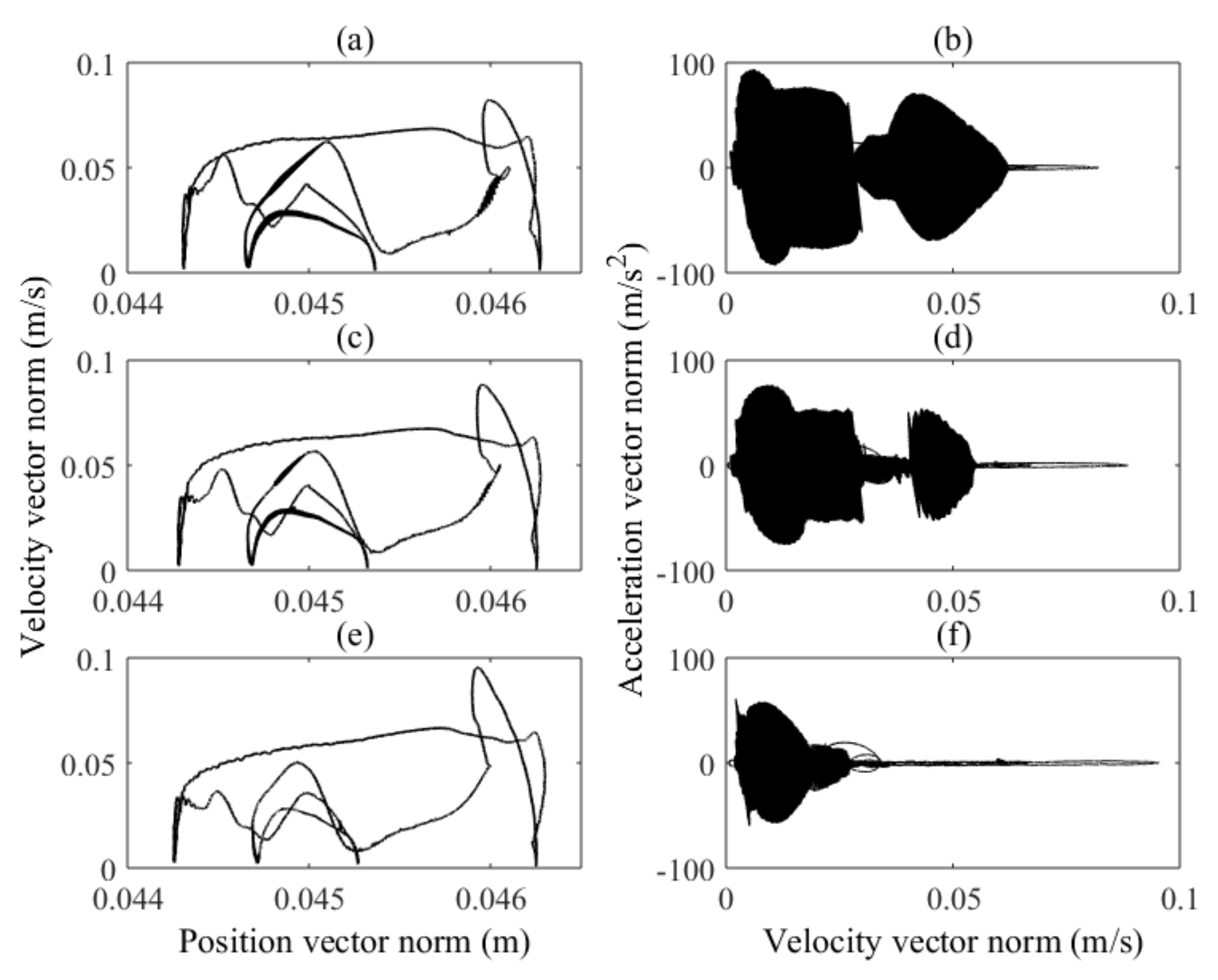
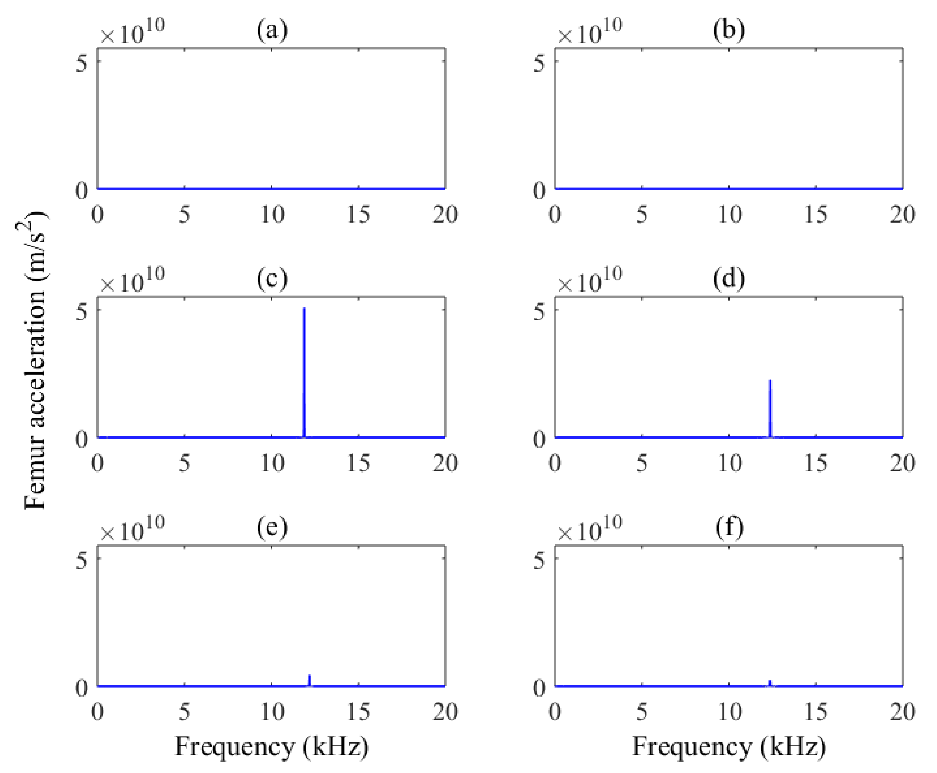
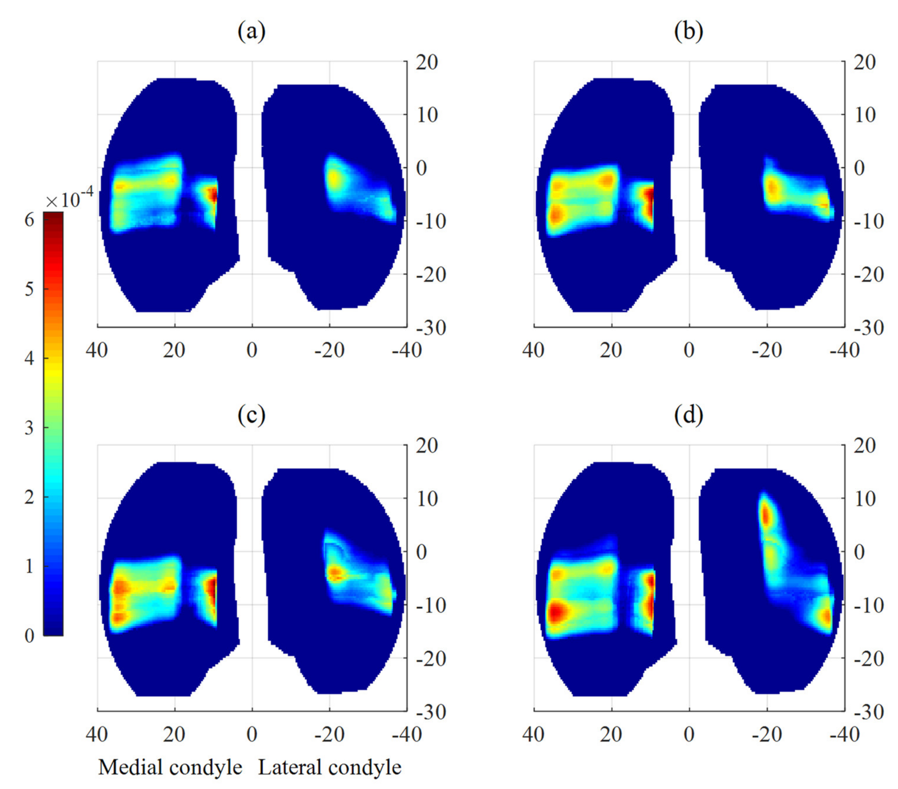
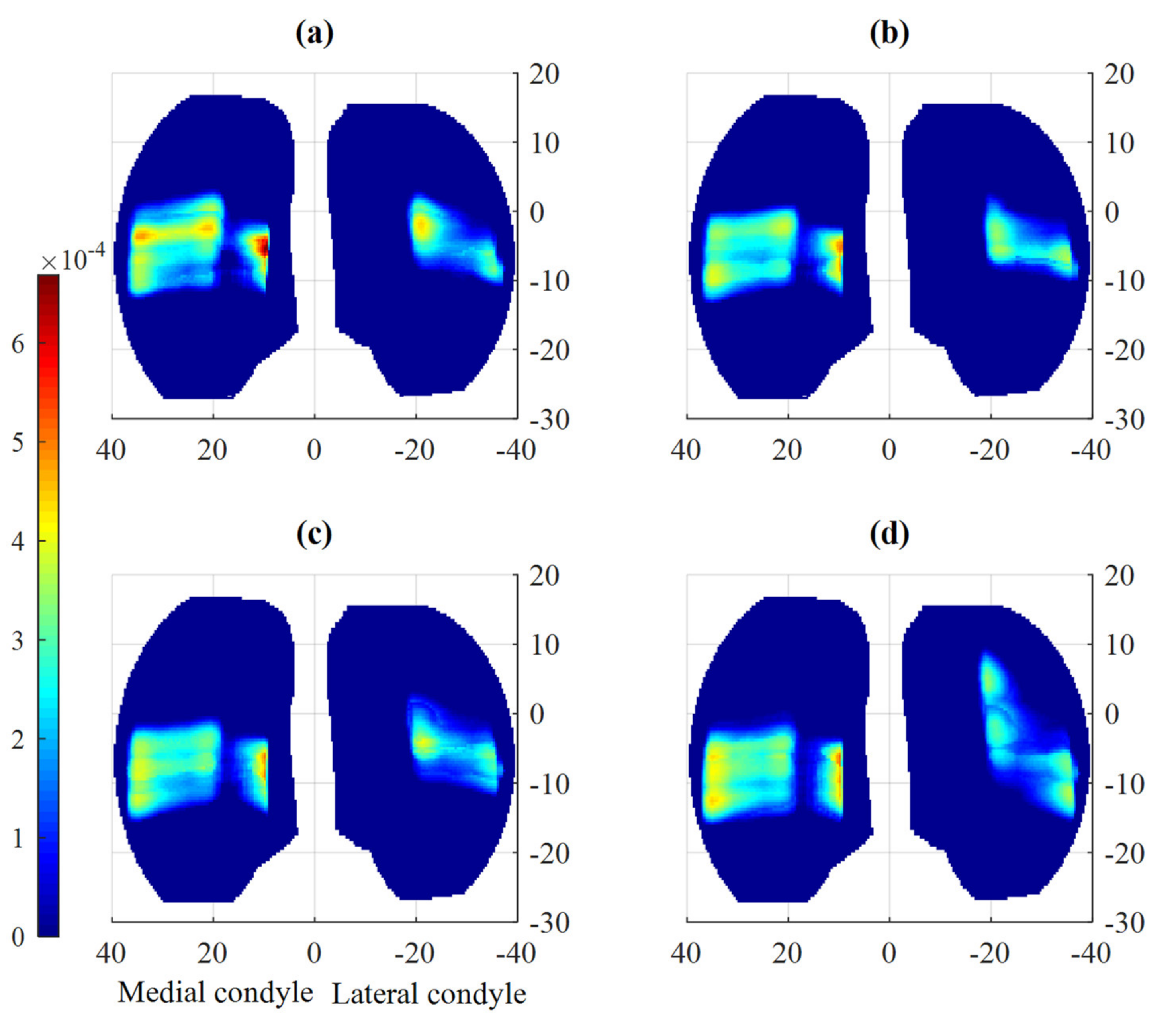
This study developed a spatial dynamic methodology to investigate the effect of friction on nonlinear dynamics, vibration, wear, and creep of tibiofemoral joints. A mesh density analysis was performed to end up with a fine mesh size that guarantees the accuracy of obtained outcomes. Comparing acquired results to those available in the literature also made it possible to evaluate the developed model. In conclusion, friction can considerably influence the motion and damage of TKAs. From the phase portrait diagrams, chaotic behaviors were observed in the tibiofemoral movement. It was also inferred that friction-induced vibration takes place when the friction coefficient increases. Moreover, using an empirical friction model resulted in vibration occurrence. Making any changes in the magnitudes of parameters in the Stribeck friction model led to the alteration of wear rates on both condyles. Furthermore, it cannot be expected that increasing the friction coefficient can always cause wear to rise owing to the strong nonlinearities of the wear mechanism. The three wear models employed in this study to predict the wear of TKAs also produced outcomes with significant differences, which should be taken into account by designers and engineers in their designing process. Eventually, it was illustrated that friction models influenced both translational and rotational loci of tibiofemoral motion, and consequently, the damage distribution.

As future research directions, the proposed model can be extended to account for the dynamics of the patella-femoral joint in addition to the tibiofemoral joint as well as to take fluid lubrication into account while handling fluid–structure interaction [105,106,107]. Moreover, the suggested approach can be utilized to optimize the design and material properties of TKAs to improve their lifetime and tribology performance, using optimization approaches such as genetic algorithm (GA) and particle swarm optimization (PSO) algorithms [108]. The friction models considered in this article are not able to capture dynamic characteristics of the friction phenomenon, e.g., pre-sliding and frictional lag. The dynamic-based friction approaches like Dahl and LuGre are to be employed accounting for these characteristics, which can lead to much more precise outcomes than those obtained in our study. As was illustrated, increasing friction leads to friction-induced vibration that should be considered in more detail experimentally as well. In addition, the viscoelasticity of polyethylene tibial insert can be considered using more sophisticated models, namely the generalized Maxwell model, Wagner model, and Prony series [109].

The present study assumed that the geometry evolution of the polyethylene tibia owing to material loss and creep deformation does not affect the contact stresses and knee trajectory, whereby the wear magnitude varies linearly during the wear analysis. Surface evolution leads to a reduction in contact stresses over time, resulting in decreasing wear rates and creep deformation [36]. Therefore, it can be deduced that the present study overestimated linear wear rates and creep deformation, both of which are dependent on contact pressure. The presented methodology can be extended to include the surface variations of the plastic tibial insert due to the wear and creep phenomena. The improved model will address the effect of the geometry update on both contact stresses and contact point trajectory, and eventually, wear and creep. Furthermore, damage distribution was found to vary with changes in the friction coefficient of knee components. Therefore, a greater area of the polyethylene tibia can get damaged when friction increases. A future direction of this research is to consider how any alteration in the damage map can influence the performance and lifetime of TKAs. The knowledge gained through such a study can contribute to the design and material development of TKAs.

References

1. Akay, A. Acoustics of friction. J. Acoust. Soc. Am. 2002, 111, 1525–1548. [Google Scholar] [CrossRef]
2. Askari, E.; Flores, P.; Dabirrahmani, D.; Appleyard, R. Dynamic modeling and analysis of wear in spatial hard-on-hard couple hip replacements using multibody systems methodologies. Nonlinear Dyn. 2015, 82, 1039–1058. [Google Scholar] [CrossRef]
3. Ren, K.; Dusad, A.; Zhang, Y.; Wang, D. Therapeutic intervention for wear debris-induced aseptic implant loosening. Acta Pharm. Sin. B 2013, 3, 76–85. [Google Scholar] [CrossRef] [Green Version]
4. Nassutt, R.; Wimmer, M.A.; Schneider, E.; Morlock, M.M. The influence of resting periods on friction in the artificial hip. Clin. Orthop. Relat. Res. 2003, 407, 127–138. [Google Scholar] [CrossRef] [PubMed]
5. Simon, S.R.; Paul, I.L.; Rose, R.M.; Radin, E.L. “Stiction-frictio” of total hip prostheses and its relationship to loosening. J. Bone Jt. Surg. Am. 1975, 57, 226–230. [Google Scholar] [CrossRef]
6. Sathasivam, S.; Walker, P. Optimization of the bearing surface geometry of total knees. J. Biomech. 1994, 27, 255–264. [Google Scholar] [CrossRef]
7. Blunn, G.W.; Lilley, P.A.; Walker, P.S. Variability of wear of ultra high molecular weight polyethylene in simulated. TKR Trans. 40th Annu. Meet Orthop. Res. Soc. 1994, 19, 177. [Google Scholar]
8. Collier, J.P.; Mayor, M.B.; McNamara, J.L.; Surprenant, V.A.; Jensen, R.E. Analysis of the failure of 122 polyethylene inserts from uncemented tibial knee components. Clin. Orthop. 1991, 273, 232–242. [Google Scholar] [CrossRef]
9. Iversen, B.F.; Stürup, J.; Jacobsen, K.; Andersen, J. Implications of muscular defense in testing for the anterior drawer sign in the knee. A stress radiographic investigation. Am. J. Sports Med. 1989, 17, 409–413. [Google Scholar] [CrossRef] [PubMed]
10. Warren, P.J.; Olanlokun, T.K.; Cobb, A.G.; Walker, P.S.; Iverson, B.F. Laxity and function in knee replacements. A comparative study of three prosthetic designs. Clin. Orthop. Relat. Res. 1994, 305, 200–208. [Google Scholar] [CrossRef]
11. Askari, E.; Flores, P.; Dabirrahmani, D.; Appleyard, R. Nonlinear vibration and dynamics of ceramic on ceramic artificial hip joints: A spatial multibody modelling. Nonlinear Dyn. 2014, 76, 1365–1377. [Google Scholar] [CrossRef]
12. Kang, L.; Galvin, A.L.; Brown, T.D.; Jin, Z.; Fisher, J. Quantification of the effect of cross-shear on the wear of conventional and highly cross-linked UHMWPE. J. Biomech. 2008, 41, 340–346. [Google Scholar] [CrossRef] [Green Version]
13. Kang, L.; Galvin, A.L.; Brown, T.D.; Fisher, J.; Jin, Z. Wear simulation of ultra-high molecular weight polyethylene hip implants by incorporating the effects of cross-shear and contact pressure. Proc. Inst. Mech. Eng. Part H J. Eng. Med. 2008, 222, 1049–1064. [Google Scholar] [CrossRef] [PubMed]
14. Wang, A.; Sun, D.C.; Yau, S.S.; Edwards, B.; Sokol, M.; Essner, A.; Polineni, V.K.; Stark, C.; Dumbleton, J.H. Orientation softening in the deformation and wear of ultra-high molecular weight polyethylene. Wear 1997, 203–204, 230–241. [Google Scholar] [CrossRef]
15. Wang, A.; Essner, A.; Polineni, V.K.; Stark, C.; Dumbleton, J.H. Lubrication and wear of ultrahigh molecular weight polyethylene in total joint replacements. Tribol. Int. 1998, 31, 17–33. [Google Scholar] [CrossRef]
16. Lee, K.Y.; Pienkowski, D. Compressive creep characteristics of extruded ultrahigh-molecular-weight polyethylene. J. Biomed. Mater. Res. 1998, 39, 261–265. [Google Scholar] [CrossRef]
17. Ramamurti, B.; Estok, D.M.; Bragdon, C.R.; Weinberg, E.A.; Jasty, M.; Harris, W.H. Dimensional changes in metal-backed polyethylene acetabular cups under cyclic loading. In Proceedings of the 45th Annual Meeting of the Orthopedic Research Society, Anaheim, CA, USA, 1–4 February 1999. [Google Scholar]
18. Davidson, J.A.; Schwartz, G. Wear, creep, and frictional heat of femoral implant articulating surfaces and the effect on long-term performance—Part I, review. J. Biomed. Mater. Res. 1987, 21, 261–285. [Google Scholar] [PubMed]
19. Persson, B.N.J. Sliding Friction, Physical Principles and Applications, 2nd ed.; Springer: Berlin/Heidelberg, Germany; New York, NY, USA, 2000. [Google Scholar]
20. Dowson, D. History of Tribology, 2nd ed.; Wiley: Hoboken, NJ, USA, 1998; ISBN 978-1-86058-070-3. [Google Scholar]
21. Popova, E.; Popov, V.L. The research works of Coulomb and Amontons and generalized laws of friction. Friction 2015, 3, 183–190. [Google Scholar] [CrossRef] [Green Version]
22. Amontons, G. De la resistance cause’e dans les machines. Mémoires de l’Academie Royale des Sciences 1699, 2, 206–226. [Google Scholar]
23. Euler, L. Sur le frottement des corps solides (On the Friction of Solid Bodies). Mémoires de l’académie des sciences de Berlin 1750, 4, 122–132. [Google Scholar]
24. Olsson, H.; Åström, K.J.; Canudas de Wit, C.; Gäfvert, M.; Lischinsky, P. Friction Models and Friction Compensation. Eur. J. Control 1998, 4, 176–195. [Google Scholar] [CrossRef] [Green Version]
25. Marques, F.; Flores, P.; Claro, J.C.P.; Lankarani, H.M. A survey and comparison of several friction force models for dynamic analysis of multibody mechanical systems. Nonlinear Dyn. 2016, 86, 1407–1443. [Google Scholar] [CrossRef]
26. Wang, A.; Essner, A.; Klein, R. Effect of contact stress on friction and wear of ultra-high molecular weight polyethylene in total hip replacement. Proc. Instn. Mech. Engrs. Part H 2001, 215, 133–139. [Google Scholar] [CrossRef]
27. Saikko, V. Effect of contact pressure on wear and friction of ultra-high molecular weight polyethylene in multidirectional sliding. Proc. Inst. Mech. Eng. Part H J. Eng. Med. 2006, 220, 723–731. [Google Scholar] [CrossRef] [PubMed] [Green Version]
28. Barceinas-Sanchez, J.D.O.; Alvarez-Vera, M.; Montoya-Santiyanes, L.A.; Dominguez-Lopez, I.; Garcia-Garcia, A.L. The coefficient of friction of UHMWPE along an entire walking cycle using a ball-on-disc tribometer under arthrokinematics and loading conditions prescribed by ISO 14243-3:2014. J. Mech. Behav. Biomed. Mater. 2017, 65, 274–280. [Google Scholar] [CrossRef]
29. Garcia-Garcia, A.L.; Alvarez-Vera, M.; Montoya-Santiyanes, L.A.; Dominguez-Lopez, I.; Montes-Seguedo, J.L.; Sosa-Savedra, J.C.; Barceinas-Sanchez, J.D.O. Regression models to predict the behavior of the coefficient of friction of AISI 316L on UHMWPE under ISO 14243-3 conditions. J. Mech. Behav. Biomed. Mater. 2018, 82, 248–256. [Google Scholar] [CrossRef]
30. Montes-Seguedo, J.L.; Garcia-Garcia, A.L.; Barceinas-Sanchez, J.D.O.; Sosa-Savedra, J.C.; Morales-Garcia, M.R.J.; Gonzalez-Jasso, E.; Dominguez-Lopez, I. Mapping the friction coefficient of AISI 316L on UHMWPE lubricated with bovine serum to study the effect of loading and entrainment at high values of sliding-to-rolling ratio. Health Technol. 2020, 10, 385–390. [Google Scholar] [CrossRef]
31. Wriggers, O. Computational Contact Mechanics, 2nd ed.; Springer: Berlin/Heidelberg, Germany, 2006. [Google Scholar]
32. Sathasivam, S.; Walker, P.S. A computer model with surface friction for the prediction of total knee kinematics. J. Biomech. 1997, 30, 177–184. [Google Scholar] [CrossRef]
33. Fisher, J.; Dowson, D. Tribology of totai artificial joints. Proc. Insr. Mech. Engrs. 1991, 205, 73–79. [Google Scholar] [CrossRef]
34. Wismans, J.; Veldpaus, F.; Janssen, J.; Huson, A.; Strulen, P. A threedimensional mathematical model of the knee joint. J. Biomech. 1980, 13, 677–686. [Google Scholar] [CrossRef] [Green Version]
35. Marra, M.A.; Vanheule, V.; Fluit, R.; Koopman, B.; Ramussen, J.; Verdonschot, N.; Andersen, M.S. A Subject-Specific Musculoskeletal Modeling Framework to Predict In Vivo Mechanics of Total Knee Arthroplasty. J. Biomech. Eng. 2015, 137, 020904. [Google Scholar] [CrossRef]
36. Fregly, B.J.; Sawyera, W.G.; Harmand, M.K.; Banks, S.A. Computational wear prediction of a total knee replacement from in vivo kinematics. J. Biomech. 2005, 38, 305–314. [Google Scholar] [CrossRef]
37. Beynnon, B.; Yu, J.; Huston, D.; Fleming, B.; Johnson, R.; Haugh, L.; Pope, M.H. A sagittal plane model of the knee and cruciate ligaments with application of a sensitivity analysis. J. Biomech. Eng. 1996, 118, 227–239. [Google Scholar] [CrossRef] [PubMed]
38. Koh, Y.G.; Lee, J.A.; Lee, H.Y.; Kim, H.J.; Kang, K.T. Computational wear prediction of insert conformity and material on mobile-bearing unicompartmental knee arthroplasty. Bone Jt. Res. 2019, 8, 563–569. [Google Scholar] [CrossRef]
39. Andriacchi, T.P. Dynamics of knee malalignment. Orthop. Clin. N. Am. 1994, 25, 395–403. [Google Scholar] [CrossRef]
40. Bei, Y.; Fregly, B.J. Multibody dynamic simulation of knee contact mechanics. Med. Eng. Phys. 2004, 26, 777–789. [Google Scholar] [CrossRef] [Green Version]
41. Pandy, M.G.; Sasaki, K.; Kim, S. A Three-dimensional musculoskeletal model of the human knee joint. Part 1: Theoretical construction. Comput. Methods Biomech. Biomed. Eng. 1997, 1, 87–108. [Google Scholar] [CrossRef]
42. Moeinzadeh, M.H.; Engin, A.E.; Akkas, N. Two-dimensional dynamic modeling of human knee joint. J. Biomech. 1983, 16, 253–264. [Google Scholar] [CrossRef]
43. Engin, A.E.; Moeinzadeh, M.H. Dynamic modelling of human articulating joints. Math. Model. 1983, 4, 117–141. [Google Scholar] [CrossRef] [Green Version]
44. Wongchaisuwat, C.; Hemami, H.; Buchner, H.J. Control of sliding and rolling at natural joints. ASME J. Biomech. Eng. 1984, 106, 368–375. [Google Scholar] [CrossRef]
45. Tumer, S.T.; Wang, X.; Akkas, N. A planar dynamic anatomical model of the human lower limb. Biomed. Eng. Appl. Basis Commun. 1995, 7, 365–378. [Google Scholar]
46. Abdel-Rahman, E.; Hefzy, M.S. A two-dimensional dynamic anatomical model of the human knee joint. ASME J. Biomech. Eng. 1993, 115, 357–365. [Google Scholar] [CrossRef]
47. Ling, Z.K.; Guo, H.Q.; Boersma, S. Analytical study on the kinematic and dynamic behaviors of a knee joint. Med. Eng. Phys. 1997, 19, 29–36. [Google Scholar] [CrossRef]
48. Tumer, S.T.; Engin, A.E. Three-body segment dynamic model of the human knee. ASME J. Biomech. Eng. 1993, 115, 350–356. [Google Scholar] [CrossRef]
49. Abdel-Rahman, E.M.; Hefzy, M.S. Three-dimensional dynamic behavior of the human knee joint under impact loading. Med. Eng. Phys. 1998, 20, 276–290. [Google Scholar] [CrossRef]
50. Caruntu, D.I.; Hefzy, M.S. 3-D Anatomically based dynamic modeling of the human knee to include tibio-femoral and patello-femoral joints. J. Biomech. Eng. 2004, 126, 44–53. [Google Scholar] [CrossRef] [PubMed]
51. Askari, E.; Andersen, M.S. Effect of ligament properties on nonlinear dynamics and wear prediction of knee prostheses. J. Biomech. Eng. 2021, 143, 021014. [Google Scholar] [CrossRef]
52. Piazza, S.J.; Delp, S.L. Three-dimensional simulation of total knee replacement motion during a step-up task. J. Biomech. Eng. 2001, 123, 599–606. [Google Scholar] [CrossRef]
53. Andersson, S.; Söderberg, A.; Björklund, S. Friction models for sliding dry, boundary and mixed lubricated contacts. Tribol. Int. 2007, 40, 580–587. [Google Scholar] [CrossRef]
54. Reynolds, O. On the Theory of Lubrication and its application to Mr. Beauchamp tower’s experiments, including an experimental determination of the viscosity of olive oil. Philos. Trans. R. Soc. Lond. 1886, 177, 157–234. [Google Scholar]
55. Stribeck, R. Die wesentlichen Eigenschaften der Gleitund Rollenlager: (The key qualities of sliding and roller bearings). Z. Vereines Deutsch. Ingen. 1902, 46, 1342–1348. [Google Scholar]
56. Panovko, Y.G.; Gubanova, I.I. Stability and Oscillations of Elastic Systems, Paradoxes, Fallacies, and New Concepts; Consultants Bureau Enterprises: New York, NY, USA, 1965. [Google Scholar]
57. Ibrahim, R.A. Friction-induced vibration, chatter, squeal, and chaos. Part I: Mechanics of contact and friction. Appl. Mech. Rev. 1994, 47, 209–226. [Google Scholar] [CrossRef]
58. Armstrong-Hélouvry, B. Control of Machines with Friction; Kluwer: Boston, MA, USA, 1991. [Google Scholar]
59. Kragel’skii, I.V. Friction and Wear; Butterworths: London, UK, 1965. [Google Scholar]
60. Kragel’skii, I.V.; Dobychin, M.N.; Kombalov, V.S. Friction and Wear: Calculation Methods; Pergamon Press: Oxford, UK, 1982. [Google Scholar]
61. Bengisu, M.T.; Akay, A. Stability of friction-induced vibrations in multi-degree-of-freedom systems. J. Sound Vib. 1994, 171, 557–570. [Google Scholar] [CrossRef]
62. Kanga, J.; Krousgrilla, C.M.; Sadeghi, F. Oscillation pattern of stick-slip vibrations. Int. J. Non-Linear Mech. 2009, 44, 820–828. [Google Scholar] [CrossRef]
63. Karnopp, D. Computer simulation of slip-stick friction in mechanical dynamic systems. J. Dyn. Syst. Meas. Control. 1985, 107, 100–103. [Google Scholar] [CrossRef]
64. Gaul, L.; Nitsche, R. The role of friction in mechanical joints. Appl. Mech. Rev. 2001, 54, 93–106. [Google Scholar] [CrossRef]
65. Canudas de Wit, C.; Olsson, H.; Astrom, K.J.; Lischinsky, P. New model for control of systems with friction. IEEE Trans. Autom. Control. 1995, 40, 419–425. [Google Scholar] [CrossRef] [Green Version]
66. Dahl, P.R. A Solid Friction Model; Technical Report TOR-0158(3107-18)-1; The Aerospace Corporation: El Segundo, CA, USA, 1968. [Google Scholar]
67. Dankowicz, H. On the modeling of dynamic friction phenomena. ZAMM J. Appl. Math. Mech. Z. Angew. Math. Mech. 1999, 79, 399–409. [Google Scholar] [CrossRef]
68. Bauchau, O.A. Flexible Multibody Dynamics; Springer: Berlin/Heidelberg, Germany, 2011. [Google Scholar]
69. Askari, E. Mathematical models for characterizing non-Hertzian contacts. Appl. Math. Model. 2021, 90, 432–447. [Google Scholar] [CrossRef]
70. Johnson, K.L. Contact Mechanics; Cambridge University Press: Cambridge, UK, 1985. [Google Scholar]
71. Kerr, A.D. Elastic and viscoelastic foundation models. J. Appl. Mech. 1964, 31, 491–498. [Google Scholar] [CrossRef]
72. Younesian, D.; Hosseinkhani, A.; Askari, H.; Esmailzadeh, E. Elastic and viscoelastic foundations: A review on linear and nonlinear vibration modeling and applications. Nonlinear Dyn. 2019, 97, 853–895. [Google Scholar] [CrossRef]
73. Gilardi, G.; Sharf, I. Literature survey of contact dynamics modelling. Mech. Mach. Theory 2002, 37, 1213–1239. [Google Scholar] [CrossRef]
74. Põdra, P.; Andersson, S. Wear simulation with the Winkler surface model. Wear 1997, 207, 79–85. [Google Scholar] [CrossRef]
75. Zhang, J.; Chena, Z.; Wang, L.; Lia, D.; Jin, Z. A patient-specific wear prediction framework for an artificial knee joint with coupled musculoskeletal multibody-dynamics and finite element analysis. Tribol. Int. 2017, 109, 382–389. [Google Scholar] [CrossRef] [Green Version]
76. Zhao, D.; Sakoda, H.; Sawyer, W.G.; Banks, S.A.; Fregly, B.J. Predicting knee replacement damage in a simulator machine using a computational model with a consistent wear factor. J. Biomech. Eng. 2008, 130, 011004. [Google Scholar] [CrossRef] [Green Version]
77. Abdelgaied, A.; Liu, F.; Brockett, C.; Jennings, L.; Fisher, J.; Jin, Z. Computational wear prediction of artificial knee joints based on a new wear law and formulation. J. Biomech. 2011, 44, 1108–1116. [Google Scholar] [CrossRef] [PubMed]
78. Fregly, B.J.; Besier, T.F.; Lloyd, D.G.; Delp, S.L.; Banks, S.A.; Pandy, M.G.; D’Lima, D.D. Grand challenge competition to predict in vivo knee loads. J. Orthop. Res. 2012, 30, 503–513. [Google Scholar] [CrossRef] [PubMed] [Green Version]
79. Kirking, B.; Krevolin, J.; Townsend, C.; Colwell, C.W.; D’Lima, D.D. A Multiaxial Force-Sensing Implantable Tibial Prosthesis. J. Biomech. 2006, 39, 1744–1751. [Google Scholar] [CrossRef]
80. D’Lima, D.D.; Townsend, C.P.; Arms, S.W.; Morris, B.A.; Colwell, C.W. An Implantable Telemetry Device to Measure Intra-Articular Tibial Forces. J. Biomech. 2005, 38, 299–304. [Google Scholar] [CrossRef]
81. Askari, E.; Cengiz, I.F.; Alves, J.L.; Henriques, B.; Flores, P.; Fredel, M.C.; Reis, R.L.; Oliveira, J.M.; Silva, F.S.; Mesquita-Guimarães, J. Micro-CT based finite element modelling and experimental characterization of the compressive mechanical properties of 3-D zirconia scaffolds for bone tissue engineering. J. Mech. Behav. Biomed. Mater. 2020, 102, 103516. [Google Scholar] [CrossRef]
82. Askari, E.; Andersen, M.S. A modification on velocity terms of Reynolds equation in a spherical coordinate system. Tribol. Int. 2019, 131, 15–23. [Google Scholar] [CrossRef] [Green Version]
83. Askari, E.; Andersen, M.S. A closed-form formulation for the conformal articulation of metal-on-polyethylene hip prostheses: Contact mechanics and sliding distance. Proc. Inst. Mech. Eng. Part H J. Eng. Med. 2018, 232, 1196–1208. [Google Scholar] [CrossRef] [PubMed] [Green Version]
84. Askari, E.; Flores, P.; Dabirrahmani, D.; Appleyard, R. A computational analysis of squeaking hip prostheses. ASME J. Comput. Nonlinear Dyn. 2015, 10, 024502. [Google Scholar] [CrossRef] [Green Version]
85. Blankevoort, L.; Kuiper, J.H.; Huiskes, R.; Grootenboer, H.J. Articular Contact in a Three-Dimensional Model of the Knee. J. Biomech. 1991, 24, 1019–1031. [Google Scholar] [CrossRef] [Green Version]
86. Butler, D.L.; Kay, M.D.; Stouffer, D.C. Comparison of material properties in fascicle-bone units from human patellar tendon and knee ligaments. J. Biomech. 1986, 19, 425–432. [Google Scholar] [CrossRef]
87. Bowman, K.F.; Sekiya, J.K. Anatomy and Biomechanics of the Posterior Cruciate Ligament, Medial and Lateral Sides of the Knee. Sports Med. Arthrosc. 2010, 18, 222–229. [Google Scholar] [CrossRef] [PubMed]
88. Chwaluk, A.; Ciszek, B. Anatomy of the Posterior Cruciate Ligament. Folia Morphol. 2009, 68, 8–12. [Google Scholar]
89. Dimas, E.; Briassoulis, D. 3D geometric modelling based on NURBS: A review. Adv. Eng. Softw. 1999, 30, 741–751. [Google Scholar] [CrossRef]
90. Landon, R.L.; Hast, M.W.; Piazza, S.J. Robust contact modeling using trimmed NURBS surfaces for dynamic simulations of articular contact. Comput. Methods Appl. Mech. Engrg. 2009, 198, 2339–2346. [Google Scholar] [CrossRef]
91. Archard, J.F. Contact and rubbing of flat surfaces. J. Appl. Phys. 1953, 24, 981–988. [Google Scholar] [CrossRef]
92. Askari, E.; Andersen, M.S. A dynamic model of polyethylene damage in dry total hip arthroplasties: Wear and creep. Multibody Syst. Dyn. 2019, 45, 403–429. [Google Scholar] [CrossRef] [Green Version]
93. Kang, L.; Galvin, A.L.; Fisher, J.; Jin, Z. Enhanced computational prediction of polyethylene wear in hip joints by incorporating cross-shear and contact pressure in additional to load and sliding distance: Effect of head diameter. J. Biomech. 2009, 42, 912–918. [Google Scholar] [CrossRef] [PubMed]
94. Turell, M.; Wang, A.; Bellare, A. Quantification of the effect of cross-path motion on the wear rate of ultra-high molecular weight polyethylene. Wear 2003, 255, 1034–1039. [Google Scholar] [CrossRef]
95. Goreham-Voss, C.M.; Hyde, P.J.; Hall, R.M.; Fisher, J.; Brown, T.D. Cross shear implementation in sliding-distance coupled finite element analysis of wear in metal-on-polyethylene total joint arthroplasty: Intervertebral total disc replacement as an illustrative application. J. Biomech. 2010, 43, 1674–1681. [Google Scholar] [CrossRef] [Green Version]
96. Mattei, L.; Di Puccio, F.; Ciulli, E. A comparative study of wear laws for soft-on-hard hip implants using a mathematical wear model. Tribol. Int. 2013, 63, 66–77. [Google Scholar] [CrossRef]
97. Hamilton, M.A.; Sucec, M.C.; Fregly, B.J.; Banks, S.A.; Sawyer, W.G. Quantifying multidirectional sliding motions in total knee replacements. J. Tribol. 2005, 127, 280–286. [Google Scholar] [CrossRef] [Green Version]
98. Askari, E.; Jeong, K.H.; Amabili, M. Hydroelastic vibration of circular plates immersed in a liquid-filled container with free surface. J. Sound Vib. 2013, 332, 3064–3085. [Google Scholar] [CrossRef]
99. Gill, H.S.; Waite, J.C.; Short, A.; Kellert, C.F.; Price, A.J.; Murray, D.W. In vivo measurement of volumetric wear of a total knee replacement. Knee 2006, 13, 312–317. [Google Scholar] [CrossRef]
100. Lavernia, C.J.; Sierra, R.J.; Hungerford, D.S.; Krackow, K. Activity level and wear in total knee arthroplasty. A study of autopsy retrieval specimens. J. Arthroplast. 2001, 16, 446–453. [Google Scholar] [CrossRef] [Green Version]
101. Galvin, A.L.; Kang, L.; Udofia, I.; Jennings, L.M.; McEwen, H.M.; Jin, Z.; Fisher, J. Effect of conformity and contact stress on wear in fixed-bearing total knee prostheses. J. Biomech. 2009, 42, 1898–1902. [Google Scholar] [CrossRef] [PubMed]
102. Harman, M.K.; Banks, S.A.; Hodge, W.A. Polyethylene Damage and Knee Kinematics After Total Knee Arthroplasty. Clin. Orthop. Relat. Res. 2001, 392, 383–393. [Google Scholar] [CrossRef] [PubMed]
103. Wiggins, S. Introduction to Applied Nonlinear Dynamical Systems and Chaos; Springer: New York, NY, USA, 1990. [Google Scholar]
104. Wang, A. A unified theory of wear for ultra-high molecular weight polyethylene in multi-directional sliding. Wear 2001, 248, 38–47. [Google Scholar] [CrossRef]
105. Askari, E.; Daneshmand, F. Coupled vibration of cantilever cylindrical shells partially submerged in fluids with continuous, simply connected and non-convex domain. J. Sound Vib. 2010, 329, 3520–3536. [Google Scholar] [CrossRef]
106. Askari, E.; Jeong, K.H.; Ahn, K.H.; Amabili, M. A mathematical approach to study fluid-coupled vibration of eccentric annular plates. J. Fluids Struct. 2020, 98, 103129. [Google Scholar] [CrossRef]
107. Marian, M.; Orgeldinger, C.; Rothammer, B.; Neasč, D.; Vrbka, M.; Křupka, I.; Hartl, M.; Wimmer, M.A.; Tremmel, S.; Wartzack, S. Towards the understanding of lubrication mechanisms in total knee replacements—Part II: Numerical modeling. Tribol. Int. 2021, 156, 106809. [Google Scholar] [CrossRef]
108. Askari, E.; Flores, P.; Silva, F. A particle swarm-based algorithm for optimization of multi-layered and graded dental ceramics. J. Mech. Behav. Biomed. Mater. 2018, 77, 461–469. [Google Scholar] [CrossRef] [PubMed]
109. Wagner, M. Analysis of time-dependent non-linear stress-growth data for shear and elongational flow of a low-density branched polyethylene melt. Rheol. Acta 1976, 15, 136–142. [Google Scholar] [CrossRef]
Figure 1. A diagram illustrating the workflow of the model developed throughout this study.
Applsci 11 07516 g001
Figure 2. A representation of the friction model A2 on the right-hand side and B2 on the left-hand side.
Applsci 11 07516 g002
Figure 3. Determination of the minimum distance of a node, Q T k , j , on the body 2, i.e., tibial insert, to the body 1 that is the femoral body.
Applsci 11 07516 g003
Figure 4. The effect of choosing friction model on linear wear prediction (m) of TKA using friction models (a) A1; (b) A3; (c) B1; (d) C1.
Applsci 11 07516 g004
Figure 5. The effect of the used friction model on trajectory of TKA employing friction models (a) A1; (b) B1; (c) B2; (d) B3; (e) C1.
Applsci 11 07516 g005
Figure 6. Phase space portraits for different friction models: (a,b) A1; (c,d) B1; (e,f) C1, which present the acceleration magnitude of the femoral part versus velocity and the femur velocity magnitude versus its position vector norm.
Applsci 11 07516 g006
Figure 7. FFT analysis of tibiofemoral joint using different friction models and friction coefficients: (a) Coulomb law: μc = 0.05; (b) Stribeck model: μs/μc = 0.05/0.0325; (c) model A1; (d) model B1; (e) model A2; (f) model C1.
Applsci 11 07516 g007
Figure 8. Effects of friction coefficient in Coulomb friction law (left-hand side) and both static and dynamic friction coefficients of Stribeck friction model on the trajectory of TKAs.
Applsci 11 07516 g008
Figure 9. Effect of friction coefficient on the damage of TKA after five million cycles: (a) μc = 0; (b) μc = 0.05; (c) μc = 0.1; (d) μc = 0.2.
Applsci 11 07516 g009
Figure 10. Effect of static and dynamic friction coefficients on the damage of tibiofemoral joints after five million cycles: (a) μs/μc = 0/0; (b) μs/μc = 0.05/0.0325; (c) μs/μc = 0.1/0.065; (d) μs/μc = 0.2/0.13.
Applsci 11 07516 g010