Algorithm for the Conformal 3D Printing on Non-Planar Tessellated Surfaces: Applicability in Patterns and Lattices

Abstract

In contrast to the traditional 3D printing process, where material is deposited layer-by-layer on horizontal flat surfaces, conformal 3D printing enables users to create structures on non-planar surfaces for different and innovative applications. Translating a 2D pattern to any arbitrary non-planar surface, such as a tessellated one, is challenging because the available software for printing is limited to planar slicing. The present research outlines an easy-to-use mathematical algorithm to project a printing trajectory as a sequence of points through a vector-defined direction on any triangle-tessellated non-planar surface. The algorithm processes the ordered points of the 2D version of the printing trajectory, the tessellated STL files of the target surface, and the projection direction. It then generates the new trajectory lying on the target surface with the G-code instructions for the printer. As a proof of concept, several examples are presented, including a Hilbert curve and lattices printed on curved surfaces, using a conventional fused filament fabrication machine. The algorithm’s effectiveness is further demonstrated by translating a printing trajectory to an analytical surface. The surface is tessellated and fed to the algorithm as an input to compare the results, demonstrating that the error depends on the resolution of the tessellated surface rather than on the algorithm itself.

1. Introduction

One of the most used additive manufacturing (AM) technologies is fused filament fabrication (FFF), which emerged as a prototyping process. During FFF, extruded material is deposited on a flat platform, and the 3D component is built by stacking layers that cause functional weakness. A new trend in research aims to deposit extruded material using out-of-plane trajectories, following the shape of curved surfaces rather than planar layer-by-layer printing. Non-planar printing has facilitated the fabrication of complex geometries, improving their mechanical properties.

Several terms are used in the literature to refer to non-planar printing, such as curved layer fused deposition modeling (CLFDM), curved layer fused filament fabrication (CLFFF), and curved layer fused deposition (CLFD). Path planning concepts relevant to these terms overlap in terms of following a non-planar trajectory and depositing fused material onto curved surfaces. Conformal additive manufacturing usually features direct write (DW) technologies, causing a new field related to conformal fabrication using FFF to emerge. The literature also describes the use of conformal fabrication to add fused material to uneven or non-planar surfaces via one or more different materials to refer to non-planar printing.

According to Jiang and Ma [1], the current path planning strategies for improving 3D printing are divided into three groups: (1) those that improve the printing surface’s qualities, shape accuracy, or infill patterns; (2) those that save material and/or time; and (3) those that achieve specific printed properties (e.g., mechanical, topological, or functional). Constant-depth CLFD has made a very significant contribution to increasing stiffness and strength [2]. Further, variable-depth CLFD [3,4], has improved surface finishing by reducing/eliminating the stair-stepping effect. To improve structural and mechanical properties while reducing material use, Tao and Leu [5] and McCaw and Cuan-Urquizo [6] proposed manufacturing non-planar lattices or cellular structures to serve as potential mechanical metamaterials. Depositing conductive materials on a non-planar substrate, reducing material and assembly complexity, has made functional printed electronics a reality [7]. Therefore, curved layer printing has confirmed its capability to achieve and improve manufacturing properties through non-planar slicing processes, eliminating or reducing supports, creating efficient infill pattern layouts, and depositing multi-material for heterogeneous composites.

The path planning problem for conformal printing requires that material be deposited on any target surface of a body digitally represented by a model. These digital models, created with a variety of computer-aided design (CAD) file formats, are highly important, as they contain information about raster geometry representation, density, and material. Some representations are the exclusive file formats of a company, whereas others are open-source and can be transferred between different CAD systems developers to achieve a flexible product creation value chain. CAD data may contain either of the two types of model object representation: analytic geometry or faceted geometry. Analytic geometry is produced for CAD design systems and is the preferred method for design and manufacturing processes, due to its unlimited resolution and flexibility. The most common analytic representation of a continuous surface is the non-uniform rational basis spline (NURBS), which describes curves and surfaces using mathematical functions. In contrast, faceted geometry (for a detailed explanation, see [8]) is a discrete form of geometry and comprises non-parametric representation consisting of points that connect to form a tessellation or groups of polygons (often triangles) as the boundaries of a body. As Chen et al. [9] explained, faceted geometry has limited resolution but a flexible and straightforward definition. Generating a conformal 3D printing trajectory on a tessellated surface is challenging and may be an obstacle to innovative designs since the available software for 3D printing does not support generating continuous curved trajectories on triangle-defined surfaces. Therefore, the current paper presents an algorithm that can be used to project, in a given direction, a complex printing trajectory into any surface represented by faceted geometry, such as a standard tessellation language (STL) file. The algorithm uses mathematical point-projection fundamentals to transfer a set of ordered points known a priori and that usually lay on a two-dimensional plane (not mandatory) to achieve conformal printing on a non-planar surface. In this way, patterns or lattices based on parametric curves (sinusoidal, Hilbert, hexagonal, re-entrant, etc.) are successfully, conformally printed on aleatory non-planar surfaces. The trajectory’s principal points can be generated using parametric equations, recursive functions, infill patterns or a combination of these. The algorithm optimizes the number of points projected as needed for proper curved printing, calculates the normal vector for each mapped point to be used as a tool orientation for multi-axis manufacturing systems, and generates the G-code for 3D printing. The main contribution of this work consists in the generation of the G-code for continuous printing trajectories for the fabrication of curved lattices, where the mandril or target surface does not need to be analytically represented. The algorithm was developed in Matlab™(R2018a) and can be easily implemented using other programming languages.

This present document is organized as follows: Section 2 presents a review of the relevant literature, and Section 3 presents a description of the algorithm in detail and the generation of target structures and printing trajectories. Furthermore, Section 4 presents the results of implementing the algorithm, and finally, concluding remarks and future insights are given in Section 5.

2. Literature Review

Finding solutions to path planning for manufacturing processes for classical problems, such as machining, painting, welding, polishing, et cetera, on curved surfaces, is a crucial issue, and several robust solutions already exist. Some of these fundamental approaches have been adapted for printing on curved surfaces, and new ones have arisen, such as those focused on applications in multi-axis printers or robotics, where some conditions are relevant, such as speed, smooth path, workspace, collision, and singularities avoidance. This review includes recent algorithms for path planning of non-planar printing and some of the most significant concepts behind the methods used in traditional conformal manufacturing as the basis of the subsequent methods adapted for curved layer printing.

2.1. Non-Planar Path Planning for Manufacturing

According to Chen et al. [9], multi-axis tool path planning methods can be categorized into two groups: those based on parametric CAD models (analytical geometry) and those based on tessellated CAD models (faceted geometry). A parametric surface, such as ruled or loft surfaces, is defined by two or more path curves on opposite sides of the surface joined by straight lines or a loft surface. Alternatively, faceted geometry (e.g., STL files) has the advantage of being defined with simply obtained data, such as vertices and normal vectors without any parametric structure and differential attributions [10]. According to Chen and Shi [11] and Lasemi et al. [12], the three popular methods for tool path generation in multi-axis machining are iso-parametric [13,14,15], iso-planar [16,17,18], and iso-scallop height [19,20,21]. In the iso-parametric method, the contact points along the desired path are generated directly by keeping one of the two parameters as a constant (e.g., u) and varying the other (e.g., w) [12]. The iso-parametric method may not be suitable for a compound surface consisting of a collection of surface patches [22], and its main disadvantage is that scallop heights are not constants due to differences between the Cartesian and parametric space [23,24]. Iso-planar (Cartesian) tool paths are generated by intersecting a surface S(u,w) with parallel planes ($P_1,P_2,...,P_n$) in Cartesian space. This method can be used for compound surfaces, trimmed surfaces, and tessellated surfaces [12]. One advantage of this method is its uniform interval between adjacent tool paths in the Euclidean space. The third method, named iso-scallop, is an improvement of isometric and iso-planar methods, according to Mladenović et al. [23], and it generates subsequent tool paths based on the known preceding paths. These robust path planning methods are widely used for traditional industrial tasks (e.g., machining, painting, welding, polishing, and glue dispensing) and have established the basis for consecutive methods for printing. Several methods for tool path planning on triangulated surfaces have also been explored. Some authors have proposed algorithms for triangular mesh surface parameterization methods by solving partial differential equations, as Jin et al. explained in [25]. Chen et al. [26] explained a method based on the iso-planar using a tessellated CAD model, where a bounding box is defined, and the tool path is generated by cutting the bounding box along the top and front directions. Jun et al. [27] generated paths for machining from an STL by offsetting the polyhedral model and intersecting the offset surface with drive planes. Similarly, Lauwers et al. [28] and Mineo et al. [29] developed a 5-axis milling tool path generation based on faceted models consisting of contact points at the intersection of a set of parallel planes and the edges of the triangles. Lauwers et al. [28] calculated the normal vector at a given point as the average of the neighborhood triangles’ normal.

2.2. Non-Planar Path Planning for 3D Printing

The term curved layer printing and its variants mainly refer to slicing a model using curved layers instead of the traditional planar layer slicing or a combination of planar and curved. A very complete review of planar and non-planar slicing methods and path planning for AM is presented by Zhao and Guo [30]. Different approaches are also found in the literature related to conformal printing on non-planar surfaces that are not commonly associated with the curved slicing model, but which are included here due to their importance in this study. The term CLFDM was first introduced by Chakraborty et al. [31] who formulated a theoretical method, mainly based on CNC traditional concepts, for the manufacturing of thin curved shells to improve the mechanical properties and reduce the stair-step effect. Their work was based on employing longer length tool paths, focused on the proper orientation of the filament and appropriate bonding between adjacent filaments. Their formulation used a parametric surface, calculated the partial derivative of it to obtain the normal vector and then generated an offset surface. The concept of CLFDM was experimentally reported by a number of researchers, such as Singamneni, Huang, and Diegel [32,33,34]. They generated the path planning (flat layers) to produce a mandril as a support structure where the curved layers were later deposited, following the contour of the part. Later, Singamneni et al. [35] improved their algorithm of the cross product of four vector by considering a vertical plane passing through three consecutive surface points. Even though all their contributions laid the foundations of experimental CLFDM, some important details about the implemented algorithms were skipped. They studied the generation/selection of data points to produce the offset curved layer directly from the G-code or M-code generated by a CAM software, and as a result, the printing trajectory was limited to those points. Some authors have developed curved layer slicing by modeling and fitting the surface using B-spline, such as Jin et al. [36], who fitted an STL mesh surface with a B-spline surface with two independent parameters (u and v). They modified the original tessellated surface to reduce the number of triangles of the STL file and then fitted the surface. The first printing path (the author recommends it to be along one of the edges of the design) defines the next paths, which are generated by a certain offset (equidistant). They reported some limitations in the processing of the part surface due to the CAD and CAM software used. Patel et al. [37] optimized the number of curved layers needed for printing by preserving the critical features. They modeled a B-spline surface using selected critical points and generated curved offset layers optimized by the application of genetic algorithms and surface-surface intersection. Their results included simulations but a nonphysical implementation. Allen and Trask [38] used a delta configuration system and generated the printing path of a surface or skin defined mathematically and a core component (infill pattern) as a matter of contrasting distinct structural or physical functions, as Llewellyn-Jones et al. [39] later also demonstrated by producing models with aesthetic and structural properties. The algorithm consisted of converting the analytical surface in a grid XY following the points in order and calculating z for dynamic movements. McCaw and Cuan Urquizo [6] presented the procedure to fabricate non-planar lattice-shells on non-planar equation-defined surfaces (parametric Bèzier surfaces of arbitrary order), whereas Cuan-Urquizo et al. [40] generated and fabricated a lattice using rectangular equations and studied the mechanical behavior when force is applied. McCaw and Cuan-Urquizo [41] presented a mathematical approach to parametrize lattices onto Bèzier surfaces to fabricate non-planar chirality lattices and studied them under cyclic loading. Conformal printing has emerged as a process to deposit silver inks on curvilinear surfaces to create conductive paths [42]; however, some recent studies were published about path planning for conformal 3D printing using FFF. Shembekar et al. [43] proposed an algorithm for conformal printing using non-planar layers and evaluated the differences in roughness between a surface finish when printed using planar layer slicing and the proposed algorithm. The algorithm aims at collision-free trajectory planning using a projection method: (1) a grid is created on the XY plane (0.5 mm spacing); (2) vertices of each triangle are projected to the XY plane; (3) specific points of the grid belong to a particular triangle; (4) the equation of the plane of the triangle is calculated from three vertices; and then (5) the z value for these points inside the triangle is calculated and mapped back to the non-planar surface. A zigzag pattern at two different angles is used to improve the finishing of the surface. Alkadi et al. [44] proposed an algorithm to locate conformally one tessellated structure onto a second tessellated surface (substrate). The algorithm achieves the following: (1) it generates a curved slicing surface by offsetting the top of the substrate; (2) it obtains the boundaries of the pattern to be printed by the intersection of the structure and the slicing surface; and (3) 2D printing patterns are projected to create 3D patterns. To achieve conformal trajectories, this algorithm has the restriction that the bottom of the 3D structure must fit the freeform substrate, and in the case of a mismatch, the free spaces are filled to connect both structures. The algorithm outputs the G-code for 3D printing. A different approach for printing quality improvement was proposed by Ahlers et al. [45], who developed an algorithm for planar and non-planar slicing. Their main contribution is the detection of the parts suitable to be printed using non-planar slicing assuring collision-free toolpaths, using a simplified printhead model defined by the maximum nonplanar angle and the maximum nonplanar height. The printing trajectories presented are focused to achieve smooth surfaces (zigzag pattern). Feng et al. [46] implemented a five-axis machine (a delta printer plus a platform rotating) and proposed an algorithm for curved layer material extrusion. Their main contribution is the reduction of the material used for the mandril to achieve conformal curved printing; hence, the printing time is also reduced. They generated a conformal surface offset and a toolpath using the geodesic distance as the shortest zigzag along the facet edges of the STL file. The path planning consisted in equidistantly offsetting the starting curves.

Most of the work published, to the best of our knowledge, about conformal-curved trajectory printing is focused on the improvement of the surface finish (reducing the stair-stepping effect) with improvement in the mechanical performance as a consequence, and a reduction in the number of layers needed for the part to be printed. Due to this, the most-used paths for curved printing are limited to zigzag or circular patterns [43,44,46]. In these works, printing paths consisted of equidistantly offsetting starting curves, which restrict the points to define the printing trajectory. A limited number of works were focused on the generation of more complex trajectories, such as those needed for the manufacturing of lattices or specific paths for the deposition of fibers or conductive materials. Complex trajectories or patterns, such as sinusoidal lattices, were reported, and these were printed on analytical surfaces (mathematically parametrized) but not using tessellated surfaces [40,41]. Complex freeforms, such as those encountered in biomedical applications (normally obtained from scanned data), may not be mathematically parametrized. Hence, approaches such as the one presented in this paper, gain relevance; any surface, parametrizable or not, could be modeled using a tessellated surface.

The review of the related literature reveals that the work where an analytical representation is obtained from points of a curved surface, also leads to the loss of key features or resolution when fitting [36]. In this way, a double source of error exists when, for instance, vertices contained in the STL file are used for calculating an analytical approximation: the intrinsic error of tessellated CAD approximation (STL file) and the error when fitting to analytical representation. In addition, the printing trajectories are limited when these must follow the points contained in the G-code/M-code generated by CAD software, or by using only the edges or vertices found in the STL file. Motivated by these limitations found in the literature, this paper is focused on the projection of complex trajectories, such as those encountered in lattices or patterns, to a tessellated surface and the corresponding G-code generation to achieve a curved architecture structure manufactured, achieving the continuous deposition of material using non-planar printing trajectories. To highlight this work contribution,

Table 1. Comparison of important aspects of reviewed authors to highlight this work contribution. A controlled mandrel means that it is mathematically parametrized. A random mandrel means that its shape is not mathematically defined. A regular trajectory is that which is usually used, e.g., zigzag or circular. Complex trajectories are those that involve periodic or fractal patterns.

Works	Geometry of mandrel: Controlled (C) or Random (R)	Experimentation	Complex (C) or Regular (R) Trajectories	Applications
				Finish improvement and Increase in Strength	Reduction of Layers	Curved Slicing Layers	Metamaterial Lattices	Conformal Printing	Avoid Support Material
Chakraborty et al. [31]	C	-	R	X	X	-	-	-	-
Singamneni et al. [35] Huang et al. [33] Diegel et al. [32,34]	C	X	R	X	-	-	-	-	-
Jin et al. [36]	R	-	R	X	-	X	-	-	-
Patel et al. [37]	C	-	R	-	X	X	-	-	-
Allen and Trask [38] Llewellyn-Jones et al. [39]	C	X	C	X	-	X	-	-	-
McCaw and Cuan-Urquizo [6,41] Cuan-Urquizo et al. [40]	C	X	C	-	-	-	X	-	-
Shembekar et al. [43]	R	X	R	X	-	-	-	-	-
Alkadi et al. [44]	R	X	R	-	-	-	-	X	-
Feng et al. [46]	R	X	R	X	X	X	-	X	X
This work	R	X	C	-	-	-	X	X	-

shows the important aspects of different works reviewed. This works fills the gap that was identified by the achievement of conformal printing of any lattice or pattern on any non-planar complex surface, via its tessellation, avoiding the need for the previous parametrization of the target surface.

3. Materials and Methods

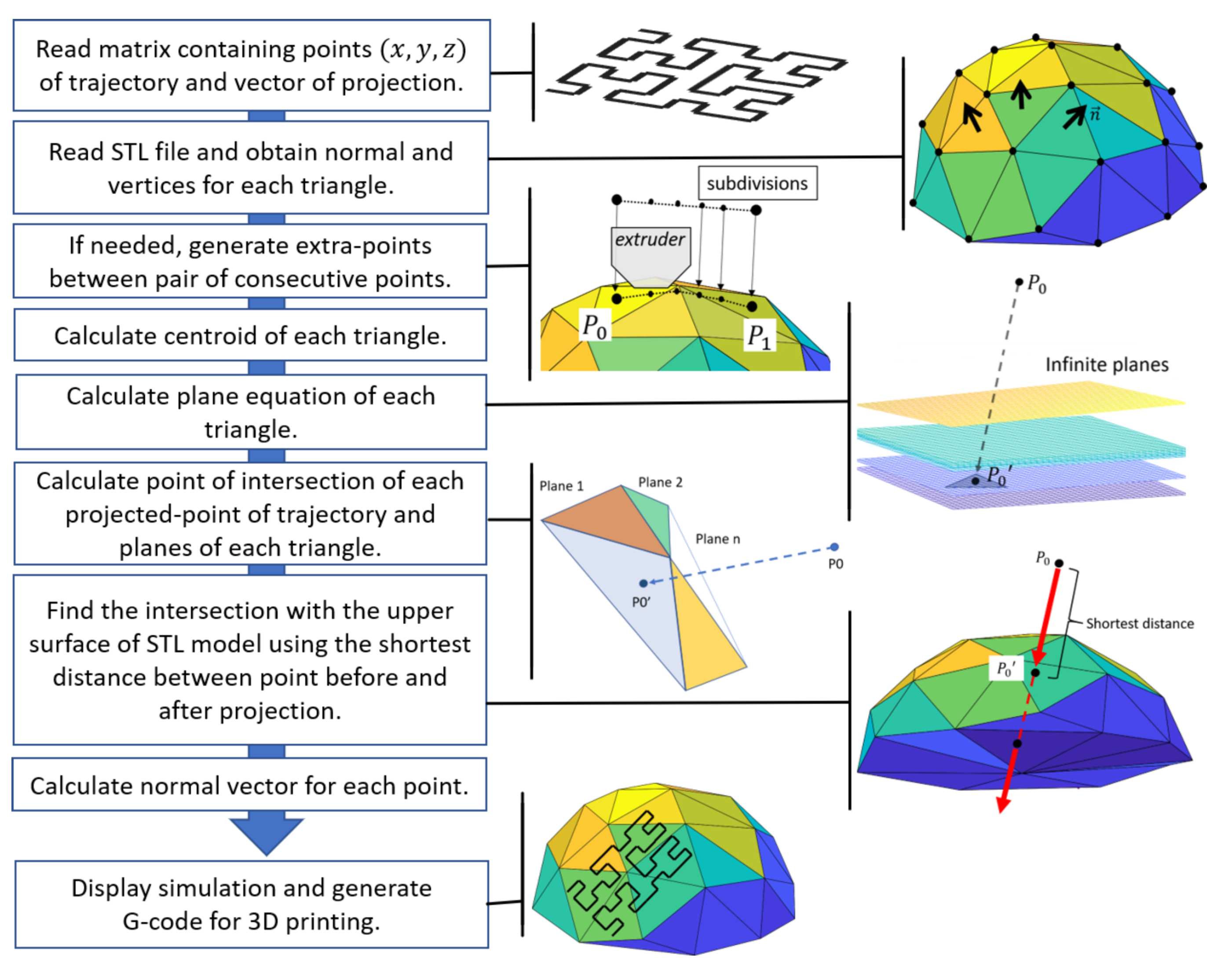
3.1. Algorithm Description

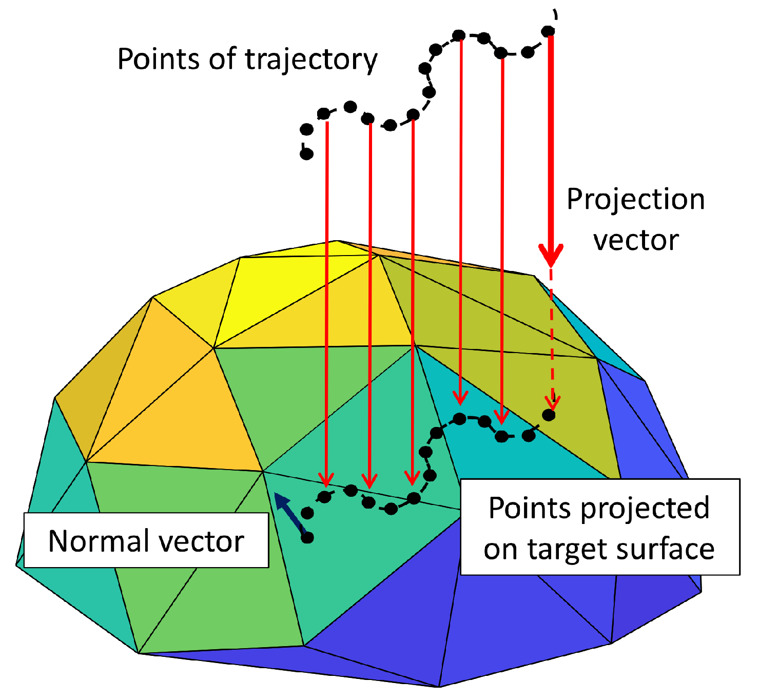
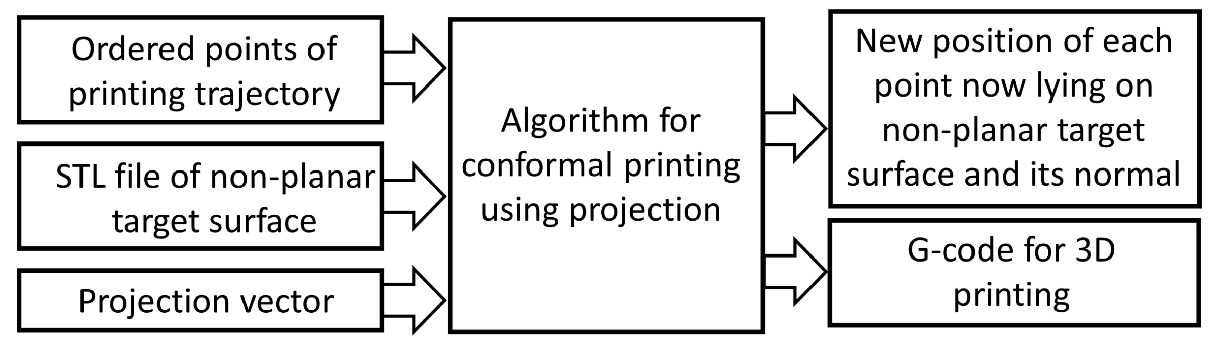
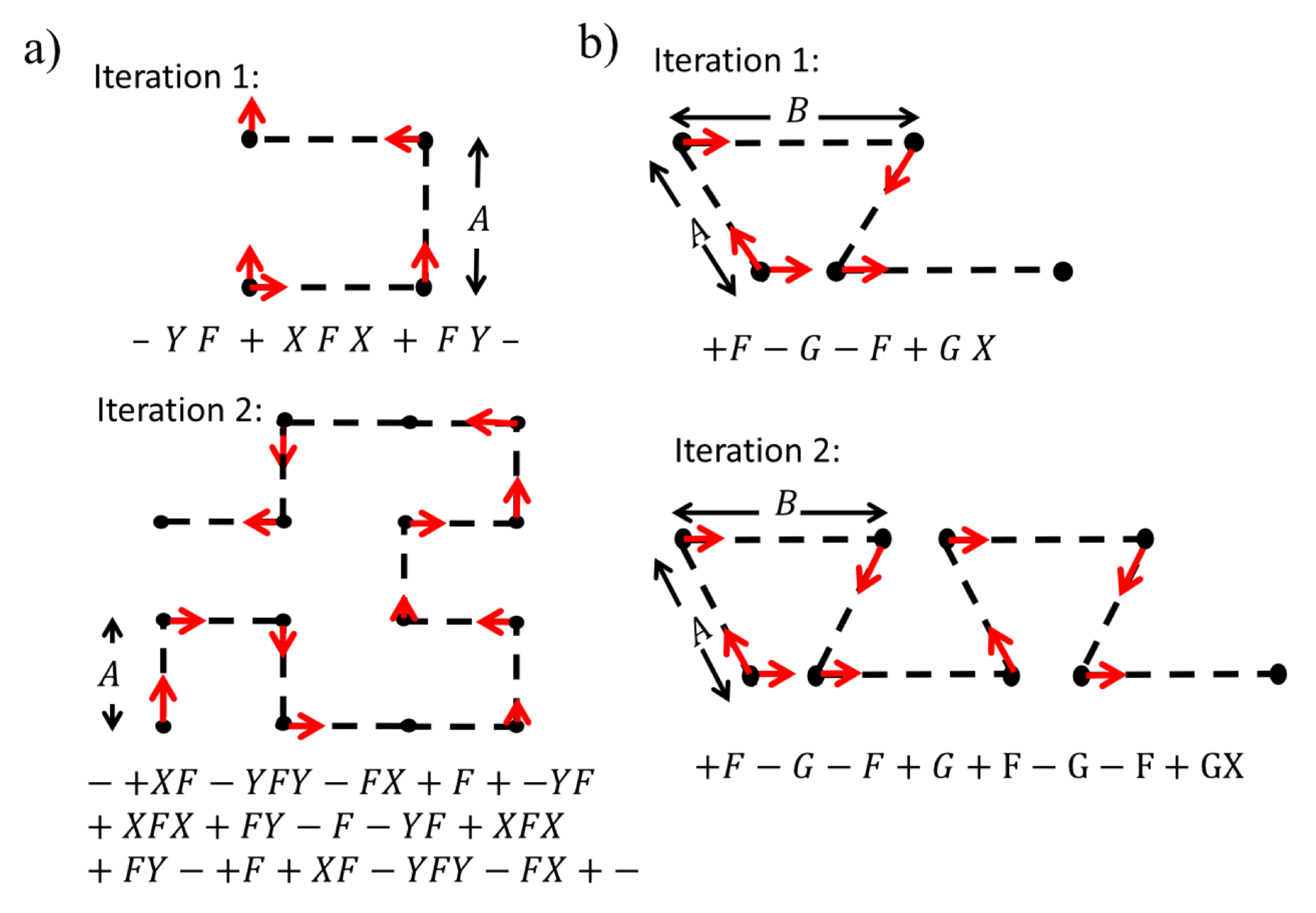
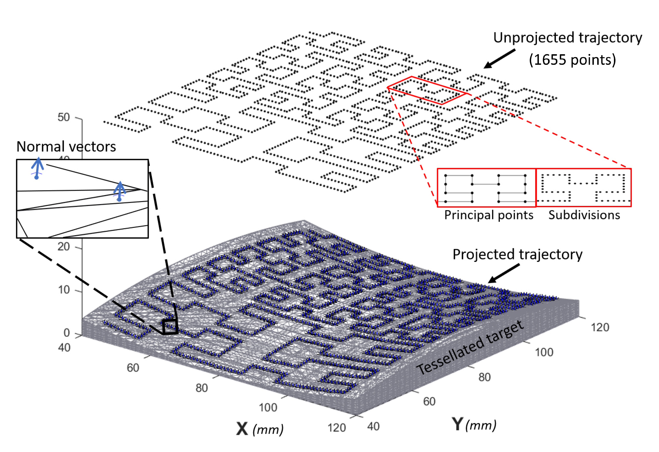
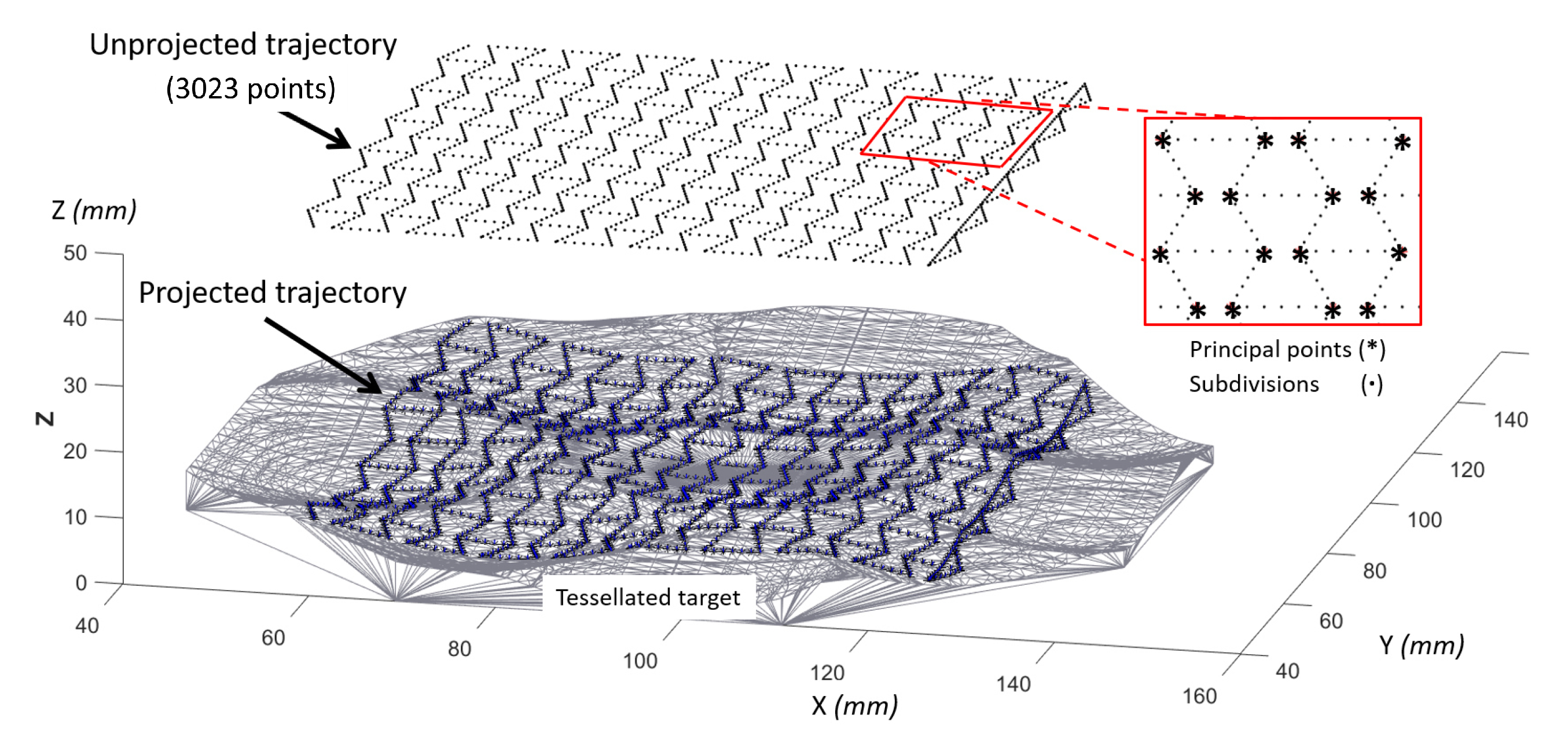
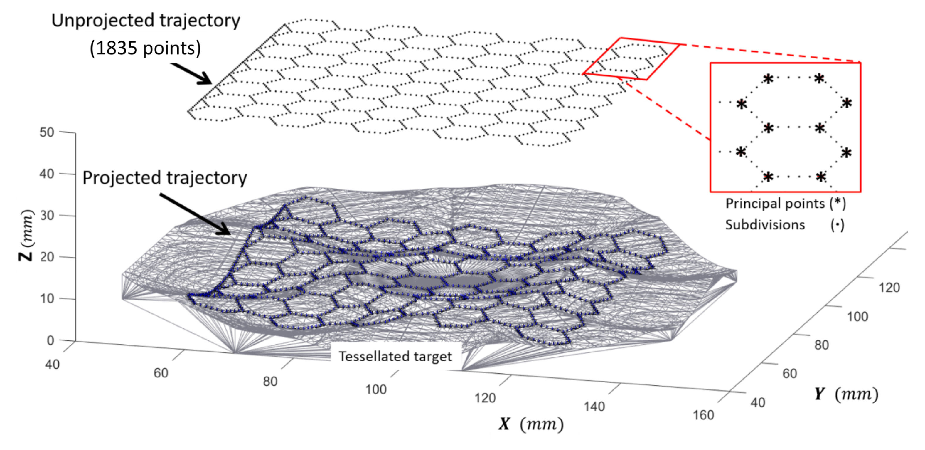
To explain the algorithm developed in this work, consider the tessellated target surface shown in Figure 1. A set of ordered points of a given trajectory are located over the target and redirected along a projection vector to intersect the surface. The intersection corresponds to each point’s new location on the target surface, and its normal is represented by the normal of the triangle where the intersection took place.

A general block diagram of the algorithm is presented in Figure 2, where three parameters are received as input:

• The coordinates $(x,y,z)$ of sequential and ordered points of the trajectory (usually lying on two-dimensional but not mandatory) are generated by parametric equations, recursive functions, or infill patterns.
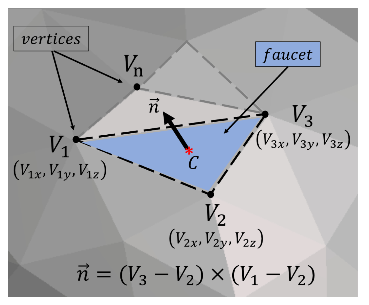
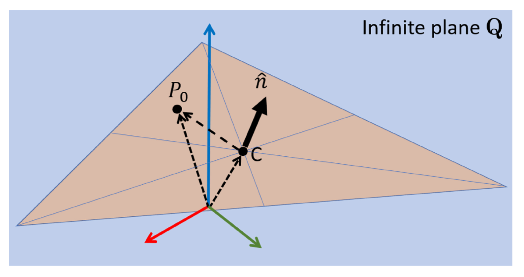
• The STL file of the non-planar target surface.
• The vector of projection (direction) of the trajectory.

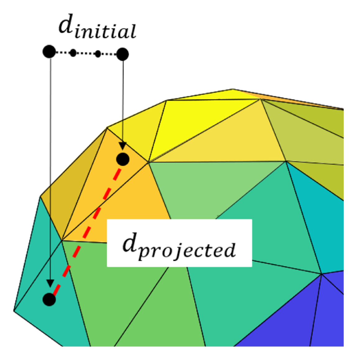
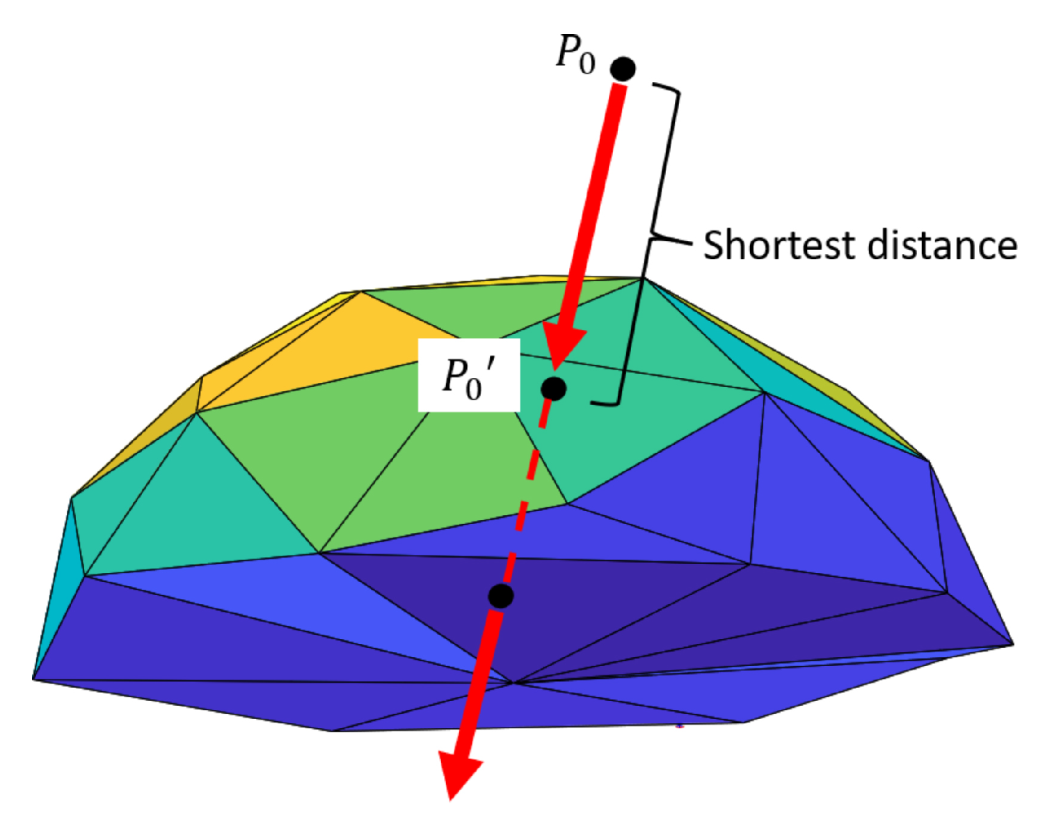
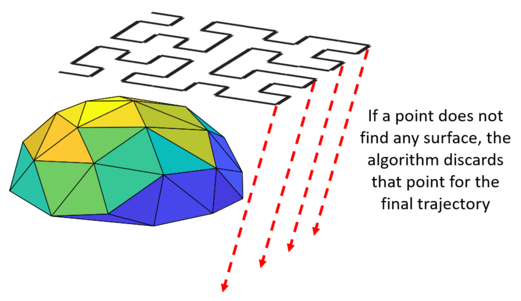
Before projection, the algorithm verifies whether the distance between each pair of consecutive points is correct for proper printing, avoiding collision with the surface when the extruder moves linearly from point to point, and if needed, the algorithm generates parametrical extra points. Then, the algorithm projects each point on the top surface and gives as output the following:

• The new position $(x,y,z)$ of every point of the path that was able to intersect the body in the given direction. The points’ sequence is maintained as it was before the projection, and those points that did not cross the body because they never found a surface are discarded.
• The normal vector for each projected point is calculated for the orientation of the extruder in the case of using a multi-axis system.
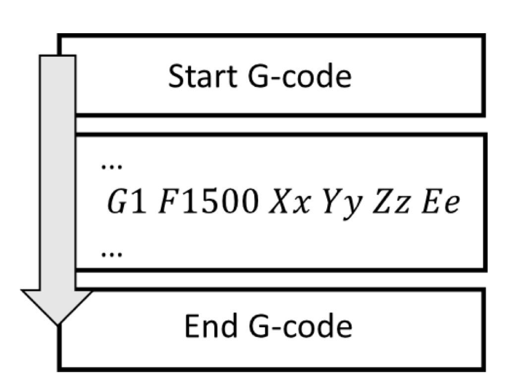
• From the new positions $(x,y,z)$, the G-code is generated for direct 3D printing.

The algorithm is detailed in the upcoming subsections (steps and definitions) and is summarized in Figure 3.

Step 1. Reading inputs:

The algorithm needs three inputs: $\left(1\right)$ a matrix containing ordered points of the trajectory, $\left(2\right)$ an STL binary file of geometry on which the points will be mapped, and $\left(3\right)$ a vector of projection. When reading the STL file, data are stored in a matrix [faces, vertices, normal] representing the triangular facets described by the $(x,y,z)$ coordinates of the three vertices and a normal unit vector. The STL file has two formats, the (i) ASCII, which is human readable, but larger (in memory) than the (ii) binary format. The normal vector is calculated using the right-hand rule (see Definition A1 in Appendix A).

Step 2. Generating extra points for smoothing the path:

The algorithm projects the points of a trajectory printing on a non-planar surface, and from these points $(x,y,z)$, the corresponding G-code is generated, which make the extruder travel in a linear fashion from point $P_i$ to $P_{i+1}$. For proper curved printing, the extruder needs to travel linearly from point to point without collisions with the target, so the distance between each point needs to be small enough to have a smooth path. Therefore, the algorithm verifies that the distance between each pair of consecutive points is correct before projecting them, and in cases where the distance is larger than $0.5$ mm or 1 mm (user-defined variable), extra points equally spaced are parametrically generated to allow the extruder to travel conformally on the curved surface without collisions, as shown in Figure 4, where the line $P_0-P_1$ needs to be subdivided before being projected for successful printing by using the parametric equation $P\left(u\right)=(1-u)P_0+u{P}_1$, where $0\le u\le 1$.

The distance between two consecutive points might change after projection since the points might cross the model at different heights (z-values) once it is projected, as shown in Figure 5.

Step 3. Calculating plane equations and centroids:

Consider a point $P_0$, which belongs to the infinite plane Q defined by a point C and a normal vector $\overrightarrow{n}$. The generalized plane’s equation for each triangle is calculated, using its normal and centroid, using the equation of a plane (see Definition A2 in Appendix A).

$$\overrightarrow{n}{P}_i+d=0$$

(1)

Therefore, taking Equation (1) for the specific case of a triangle, and if the centroid C$(c_x,c_y,c_z)$ of a triangle (defined by three vertices $(V_1,V_2,V_3)$ is calculated as $((V_{1x}+V_{2x}+V_{3x})/3$, $(V_{1y}+V_{2y}+V_{3y})/3$,$(V_{1z}+V_{2z}+V_{3z})/3\left)\right)$ and its normal vector is $\overrightarrow{n}(n_x,n_y,n_z)$, then the scalar equation of the infinite plane Q, where the three vertices and centroid of the triangle are located, is given by Equation (2):

$$n_{x}x+n_{y}y+n_{z}z+(-c_x{n}_x-c_y{n}_y-c_z{n}_z)=0$$

(2)

Step 4: Calculate the intersection of a projected point and a plane:

Consider Figure 6, where a point $P_0$ is projected in a vector direction $\overrightarrow{v}$. This infinite-line of projection can be described by its parametric equation (see Definition A3 in Appendix A).

Having described an infinite plane through Equation (2) and an infinite-line through $P=P_0+t\overrightarrow{v}$, the point of intersection between both can be found by substituting the infinite-line equation onto the infinite plane equation so that the following holds:

$$\overrightarrow{n}(P_0+t\overrightarrow{v})+d=0$$

(3)

and solving for t,

$$t=\frac{-(d+\overrightarrow{n}{P}_0)}{\overrightarrow{n}\overrightarrow{v}}$$

(4)

knowing t, the coordinates of the intersection point are calculated as follows:

$$\begin{array}{c}x=P_{0x}+t{v}_x\\ y=P_{0y}+t{v}_y\\ z=P_{0z}+t{v}_z\end{array}$$

(5)

Step 5: Finding the intersection of the projected point with true triangles:

Equation (5) is used to obtain the intersection of the projected point with the infinite plane of every triangle of the STL model, as shown in Figure 6. However, using the equation of a point inside a triangle (see Definition A4 in Appendix A), the vertices are used to delimit each triangle’s space and validate that the projected point intersects the triangles.

Step 6: Finding the intersection with the upper surface of the STL model:

Once the algorithm finds which triangles are intersected by the projected point and the location $(x,y,z)$ of the intersection, the algorithm holds the intersection only with the upper surface. When an infinite line crosses a close model, such as an object defined by an STL file, the line intersects the model at least two times; measuring the distance between the location of the point $P_0$ before projection and the intersections after projection, the shortest one, $P_0^{\prime }$, is considered the first that crosses the upper surface, as shown in Figure 7.

Step 7. Discarding those points that never intersected any surface: If a projected point does not intersect a surface to cross, then the algorithm discards the final trajectory point, as shown in Figure 8.

Step 8. Generating G-code for 3D printing:

Figure 9 shows the main parts of the generated G-code file. The start G-code prepares the printer by setting the heated bed temperature to 60 ${}^{\circ }$C and the extruder temperature to 200 ${}^{\circ }$C and purges the extruder. The end G-code finalizes the printing task by turning off the heating elements and raising the extruder. The instruction added for printing controls the extruder’s linear movements from one point to the next of the printing trajectories. Its general format is given by G1 F1500 Xx Yy Zz Ee (e.g., G1 F1500 X91.429 Y69.183 Z6.33 E0.13187), where F1500 refers to the extrusion speed (1500 mm/min), $(x,y,z)$ is the position corresponding to each projected point, and the number e is the accumulated length of the filament to be extruded. Furthermore, e is given by $\sqrt{{(x_i-x_{i-1})}^2+{(y_i-y_{i-1})}^2+{(z_i-z_{i-1})}^2}$ multiplied by a factor of $(0.4/1.75)=0.0522$.

To generate multiple layers, the initial set of points is repeated but inverted in sequence, while the z-value is increased in steps of $0.2$ mm.

3.2. Generation of Target Structures and Printing Trajectories

Two different target structures are generated with a proper slope to avoid collisions due to the restriction of a 3-axis printer:

(a) A saddle surface using Equation (6).

$$z=3.8+\frac{{\left(0.65(x-80)\right)}^2-{\left(0.65(y-80)\right)}^2}{200}$$

(6)

where $40\le x\le 120$ and $40\le y\le 120$.

(b) A random surface generated by the logical subtraction between the structure defined by Equation (7), the same structure rotated ${90}^{\circ }$ and a sphere of radius 70 mm with the center in $(95,88,73)$.

$$z=6+5(sin(x/12)cos(y/12\left)\right)$$

(7)

where $0\le x\le 32\pi$ and $0\le y\le 32\pi$.

Three different printing trajectories (Hilbert, re-entrant, and hexagonal) are generated based on the Lindenmayer system (L-system) and consist of alphabet symbols to form strings. In this method, widely explained in [47], each symbol denotes an action. Consider Figure 10a, where a Hilbert pattern has an initiation seed equal to X, where X = “-YF+XFX+FY-”, Y = “+XF-YFY-FX+”, “-” means turn right $\pi /2$ degrees, “+” means turn left $\pi /2$ degrees and “F” means go Forward A distance. Similarly, for the re-entrant curve (Figure 10b), the seed is X where X= “+F-G-F+G X”, “G” means go Forward B distance repeated N times to form a row and then M times to form the lattice. In this case, the angle of rotation is $2\pi /3$ and two different distances, F and G, are considered. A hexagonal pattern is a re-entrant pattern with distance $B=A$ and a turning angle of $\pi /3$, such as the angle for the symbols “−” and “+”.

4. Results

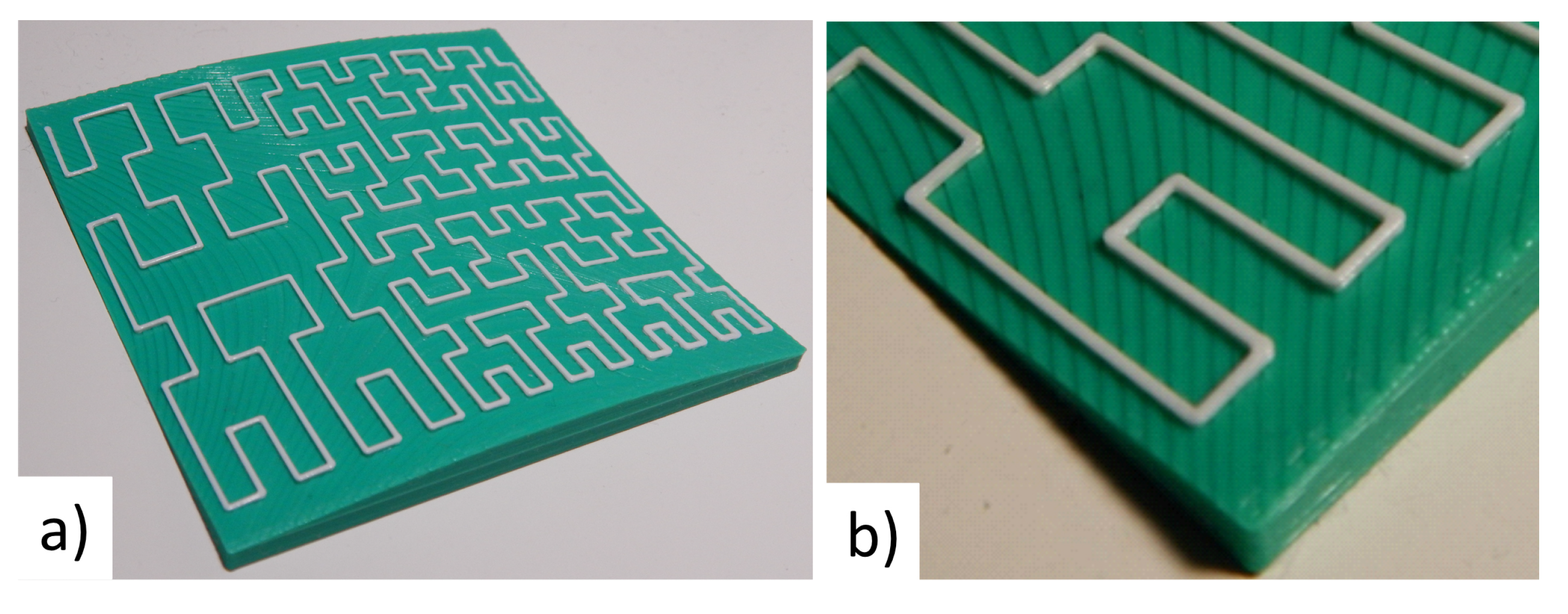
4.1. Printing of Target Structure

The two different target structures explained in Section 3.2 were designed using the software Mathematica™ and Blender, and then exported as STL files. The STL of the target model was loaded using the Software Ultimaker Cura, positioned at (40 mm, 40 mm) on the build plate, and then planar sliced, as is the traditional process, to produce the G-code for printing. An Ender-3 printer was used to print the target structures, which were the base or mandril of the subsequent conformal printing trajectories. The printer’s nozzle was 0.4 mm, and the material was a PLA filament 1.75 mm in diameter.

4.2. Printing Trajectories

The algorithm discussed in Section 3.1 was applied to project three different printing trajectories (Hilbert, re-entrant, and hexagonal). The printing trajectories and the algorithm for conformal printing were calculated in Matlab™(R2018a). The algorithm’s inputs were the STL of the target structure, the main points of each printing trajectory, and the projection vector $[0,0,-1]$, such as the -z direction. As output, the algorithm gives the new location of each point projected on the target surface and the G-code for conformal 3D printing. The printer and printing material used were the same as those for the target structure.

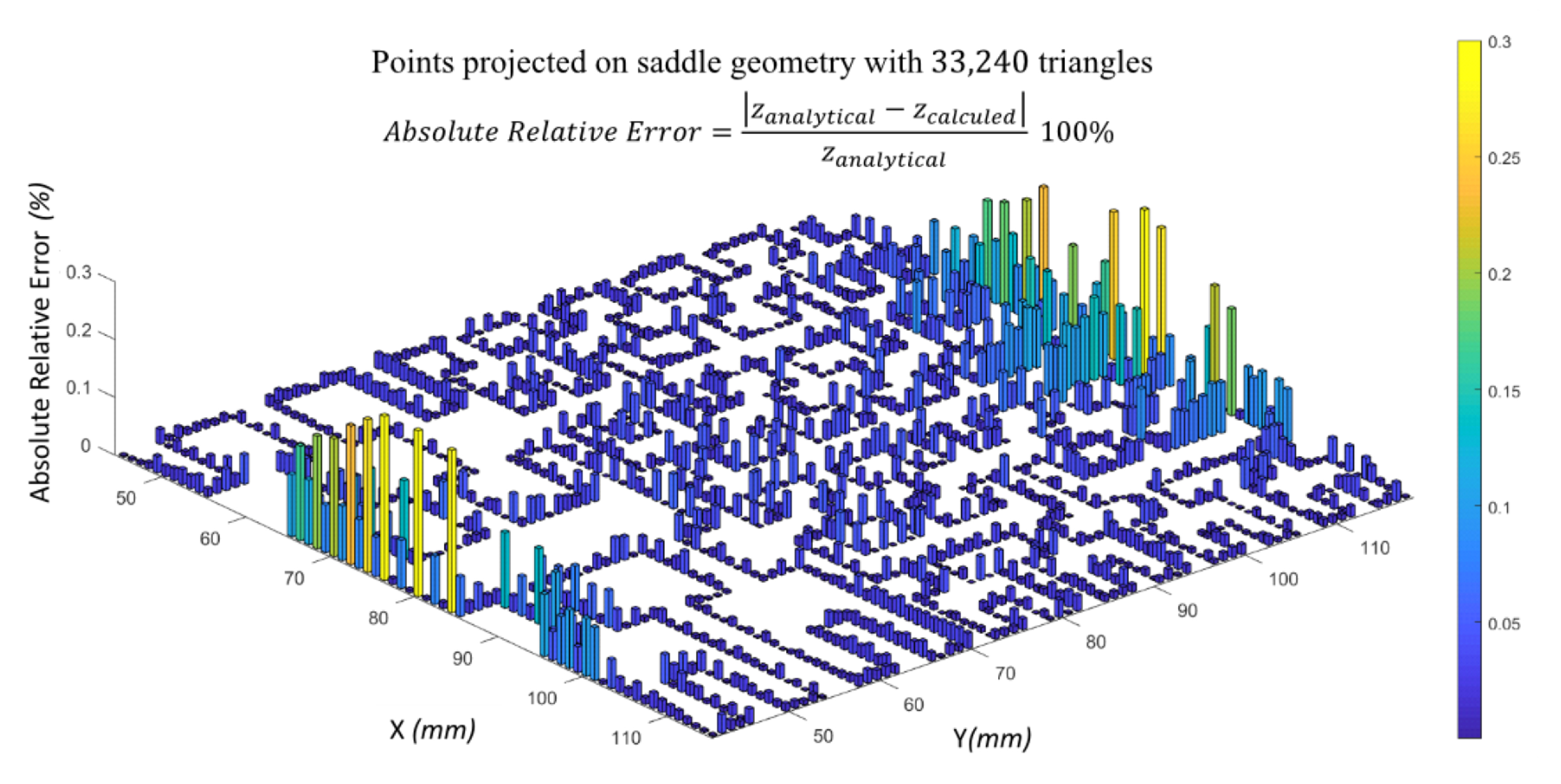
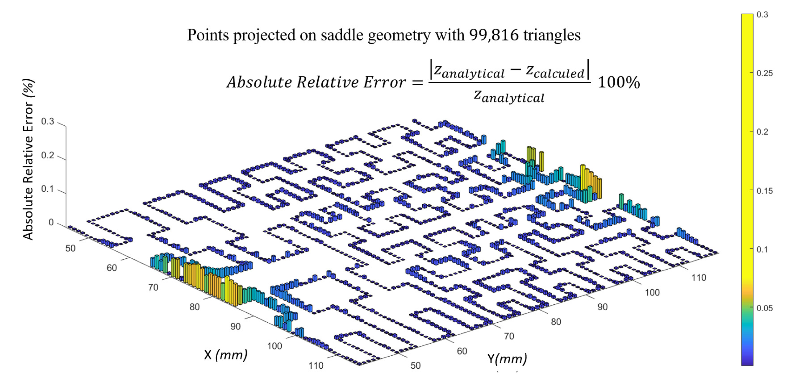
4.3. Evaluation of Algorithm

One way of demonstrating the correct functionality of the proposed algorithm is generating a printing trajectory on an analytical target surface and then comparing these values to those obtained using the algorithm by projecting the trajectory into the tessellated equivalent target surface. In this manner, the Hilbert curve explained in Section 3.2 was chosen as the printing trajectory, producing 319 principal points ordered in sequence on a XY plane $(45\le x\le 115,42\le y\le 118,z=50)$ [mm]. The target surface or mandril was chosen to be the analytical saddle surface defined by Equation (6), generated using the software Mathematica and saved as a tessellated STL file with two different resolutions: one low-resolution consisting of 33,240 triangles and another high resolution of 99,816 triangles. Having the Hilbert printing trajectory (x,y) and the curved target surface (saddle), an analytical curved printing trajectory was created by the substitution of each value (x,y) of the Hilbert pattern into the saddle surface, using Equation (6), obtaining the $Z_{analytical}$. At the same time, the algorithm for conformal printing proposed here and described in Section 3.1 was executed, having as inputs the same printing trajectory (Hilbert), the tessellated equivalent target surface (saddle STL) and a projection vector in the $-z$ direction. Before projecting the points of the printing trajectory, the algorithm generated extra points as subdivisions, having a total of 1655 sequential points for the Hilbert trajectory. The obtained algorithm output was named $Z_{projected}$ for each $(x,y)$ value. Figure 11 shows the printing trajectory before and after being conformed on the saddle surface and the normal vector for each projected point.

The absolute relative error, defined as $\frac{|Z_{analytical}-Z_{projected}|}{Z_{analytical}}100\%$, was used to measure the accuracy of the algorithm. Figure 12 shows the error found for each point $(x,y)$ of the Hilbert printing trajectory projected on the tessellated saddle structure with 33,240 triangles (low-resolution), having a mean error of $0.025853$, and a maximum error of $0.287034\%$ occurred at $(X=80,Y=42)$. Figure 13 shows the same points, but this time projected on the 99,816 triangle polygonal mesh (high-resolution structure), the mean error was $0.007551$, and the maximum error found was $0.075592\%$, which occurred at $(X=83,Y=42)$. Finally, Figure 14 shows the actual 3D-printed piece: first, the target structure (mandrel) is printed using the slicing software Cura (planar printing), then the G-code generated by the algorithm allows the continuous conformal deposition of material following the Hilbert pattern on the target structure, being noticeable the contrast between the stair-stepping effect due to the planar slicing printing process for the target structure and the conformal Hilbert curved printing trajectory.

Two lattice examples were also simulated and 3D printed. In Figure 15, a re-entrant trajectory is projected on a random target tessellated structure generated, as explained in Section 3.2, similar to that used in [43]. The re-entrant trajectory initially consisted of 432 main points that define the pattern. Additionally, the algorithm generated extra points as subdivisions to convert a linear displacement into a curve printing trajectory for the extruder, having in total 3023 points that were projected on the target surface toward the $-z$ direction. Figure 16 shows the actual printing, where the curved and continuous deposition of the extruded filament can be observed. The target structure was used to project a hexagonal trajectory, as shown in Figure 17, with 320 main points. The algorithm added extra points to achieve curved displacements, with 1835 points projected successfully on the target structure in total. The actual 3D printing of the hexagonal printing trajectory on a random structure is shown in Figure 18, where a continuous deposition of material is achieved.

5. Discussion

Lattice and cellular structures are proven to be suitable options for tailoring properties when they are used to fill parts and components. However, when characterizing their effective properties, the lattice samples are fabricated with simple macro geometries, such as cubes and prisms. Components in real applications have far from simple macro geometries. The need is then for these structures to conform to complex macro geometries. The first step toward this is to conform them to non-planar surfaces [6]. The algorithm developed in this work supports this general objective found in the literature by allowing specific trajectories (generated parametrically following recursive or repetitive patterns). Furthermore, it contributes to the manufacturing of continuous filament deposits on a non-planar surface, such as those needed for lattices (printing layer-by-layer affects the performance of structure) or to deposit conductive material (stair-stepping effect would cause discontinuity) or any second material on the surface of a substrate.

The results presented in this work demonstrate that the algorithm’s precision depends on the resolution polygonal mesh of the target structure. For example, a saddle’s geometry was chosen to use two different approximations: the first with low-resolution and 33,240 triangles, and the second with an approximately three times higher resolution (99,816 triangles). Based on the data collected and condensed in Figure 12, the mean of the absolute relative error found for the low-resolution polygonal mesh was $0.025853$, with concentrated highest values of error at the saddle surface’s concave zones and a maximum value of error of $0.287034\%$. To reduce the error, the number of triangles (vertices) must be increased to increase the polygon mesh. Here, when the resolution of the previous low-resolution polygonal mesh of saddle target was improved with approximately a three-times higher resolution geometry, the mean of the absolute relative error decreased to $0.007551$, which represents closely the same proportion $(1/3)$ of change, and the error zones remained at the concave zone, as can be observed in Figure 13. It can be assumed that the error decreases as the tessellated surface resolution improves at the same proportion. The algorithm proposed here allows for projecting complex printing trajectories to achieve structures with different densities of material as the Hilbert curve sample shown in Figure 14a, where the length of the unitary cell is changed to simulate a different density distribution. In Figure 19, the curved lattices printed were detached from the target structure, using adhesive blue painter tape to cover the target structure before printing the lattices.

6. Conclusions

This work focuses on developing a software tool to shorten the design time when conformal 3D printing is required. This consists of a mathematical algorithm to project sequential points of a trajectory through a vector for conformal printing on a tessellated surface defined by an STL file and the direct generation of the machine code (G-code) for 3D printing. The algorithm was implemented in Matlab™(R2018a), and as a proof of concept, sequential points of a Hilbert curve trajectory were generated and projected on a saddle surface to be printed conformally, using FFF. It was demonstrated that the absolute relative error between the location of the projected points using the algorithm versus the analytical values utilizing the surface’s equation was due mainly to the resolution of polygonal mesh (number of vertices in STL file) in such a way that error decreased for a tessellated surface with a higher resolution polygonal mesh. The algorithm calculates the normal vector for each projected point so that the Euler angles may be obtained to orientate a tool or extruder of a multi-axis or robotic system. The algorithm concept may be used for the generation of G-codes for printing continuous non-planar lattices or functional structures on an arbitrarily shaped and tessellated surface. The application scope may also be extended to generate G-codes for one or several layers and even by using other AM technologies, such as DW, for the deposition of conductive material for printed electronics. The algorithm was initially created for a looking solution to generate G-codes for 3D printing of conductive tracks on any surface represented by a tessellated file (STL), but its use may be extended for other surface manufacturing applications, where a path trajectory to be followed by a tool is required. Applying the algorithm for 3D printing using an industrial robot is planned for future work, including implementation of a user’s interface and some improvements to optimize calculations. The final remark of this paper concerns the advantages of using this algorithm.

• It allows projecting complex parametric trajectories onto any non-planar surfaces defined by an STL geometry file, so the surface does not have to be analytical. The generation of patterns, such as those used in [6,41] in a two-dimensional plane, is direct, but generating those patterns in 3D following a curve may be challenging if the surface is complex and not analytical.
• It allows shortening the design time and the steps for AM of conformal patterns on non-planar surfaces by directly producing a G-code to be transferred to the printing machine. It is a simple software tool that is easy to use and even modified for further specific applications.
• The algorithm gives each projected point the normal to orient the extruder in a multi-axis system.
• It allows concatenating different trajectories to create structures with different material densities.
• It allows printing as many layers as needed or alternating the pattern by layers as the sinusoidal pattern.
• Having the vector of projection as a user-defined parameter allows playing with trajectories projected at different inclination angles to generate different patterns on the target surface. Similarly, the pattern can be generated at an inclined plane and then projected as required.
• Non-planar lattice shells, when built from the projection or conformal printing, will have distortions (not present in their planar version) that will affect their resulting mechanical properties (especially if those were characterized in planar samples). This prompts further analysis of the mechanical properties of the lattice shells.

References

1. Jiang, J.; Ma, Y. Path Planning Strategies to Optimize Accuracy, Quality, Build Time and Material Use in Additive Manufacturing: A Review. Micromachines 2020, 11, 633. [Google Scholar] [CrossRef]
2. Diegel, O.; Singamneni, S.; Huang, B.; Gibson, I. Curved Layer Fused Deposition Modeling in Conductive Polymer Additive Manufacturing. Adv. Mater. Res. 2011, 199, 1984–1987. [Google Scholar] [CrossRef] [Green Version]
3. Chen, L.; Chung, M.F.; Tian, Y.; Joneja, A.; Tang, K. Variable-depth curved layer fused deposition modeling of thin-shells. Robot. Comput.-Integr. Manuf. 2019, 57, 422–434. [Google Scholar] [CrossRef]
4. Pelzer, L.; Hopmann, C. Additive manufacturing of non-planar layers with variable layer height. Addit. Manuf. 2021, 37, 101697. [Google Scholar] [CrossRef]
5. Tao, W.; Leu, M.C. Design of lattice structure for additive manufacturing. In Proceedings of the 2016 International Symposium on Flexible Automation (ISFA), Cleveland, OH, USA, 1–3 August 2016; pp. 325–332. [Google Scholar] [CrossRef]
6. McCaw, J.C.; Cuan-Urquizo, E. Curved-layered additive manufacturing of non-planar, parametric lattice structures. Mater. Des. 2018, 160, 949–963. [Google Scholar] [CrossRef]
7. Lu, B.; Lan, H.; Liu, H. Additive manufacturing frontier: 3D printing electronics. Opto-Electron. Adv. 2018, 1, 170004. [Google Scholar] [CrossRef]
8. Kai, C.C.; Jacob, G.G.K.; Mei, T. Interface Between CAD and Rapid Prototyping Systems. Part 1: A Study of Existing Interfaces. Int. J. Adv. Manuf. Technol. 1997, 13, 566–570. [Google Scholar] [CrossRef]
9. Chen, H.; Fuhlbrigge, T.; Li, X. A review of CAD-based robot path planning for spray painting. Ind. Robot. Int. J. 2009, 36, 45–50. [Google Scholar] [CrossRef]
10. Zhao, J.; Zou, Q.; Li, L.; Zhou, B. Tool path planning based on conformal parameterization for meshes. Chin. J. Aeronaut. 2015, 28, 1555–1563. [Google Scholar] [CrossRef] [Green Version]
11. Chen, T.; Shi, Z. A tool path generation strategy for three-axis ball-end milling of free-form surfaces. J. Mater. Process. Technol. 2008, 208, 259–263. [Google Scholar] [CrossRef]
12. Lasemi, A.; Xue, D.; Gu, P. A freeform surface manufacturing approach by integration of inspection and tool path generation. Int. J. Prod. Res. 2012, 50, 6709–6725. [Google Scholar] [CrossRef]
13. Broomhead, P.; Edkins, M. Generating NC data at the machine tool for the manufacture of free-form surfaces. Int. J. Prod. Res. 1986, 24, 1–14. [Google Scholar] [CrossRef]
14. Loney, G.C.; Ozsoy, T.M. NC machining of free form surfaces. Comput.-Aided Des. 1987, 19, 85–90. [Google Scholar] [CrossRef]
15. Kuragano, T. FRESDAM system for design of aesthetically pleasing free-form objects and generation of collision-free tool paths. Comput.-Aided Des. 1992, 24, 573–581. [Google Scholar] [CrossRef]
16. Bobrow, J.E. NC machine tool path generation from CSG part representations. Comput.-Aided Des. 1985, 17, 69–76. [Google Scholar] [CrossRef]
17. Chen, Y.D.; Ni, J.; Wu, S.M. Real-time CNC Tool Path Generation for Machining IGES Surfaces. J. Eng. Ind. 1993, 115, 480–486. [Google Scholar] [CrossRef]
18. Huang, Y.; Oliver, J.H. Non-constant parameter NC tool path generation on sculptured surfaces. Int. J. Adv. Manuf. Technol. 1994, 9, 281–290. [Google Scholar] [CrossRef]
19. Suresh, K.; Yang, D. Constant scallop-height machining of free-form surfaces. J. Eng. Ind. 1994, 116, 253–259. [Google Scholar] [CrossRef]
20. Lin, R.S.; Koren, Y. Efficient tool-path planning for machining free-form surfaces. J. Eng. Ind. 1996, 118, 20–28. [Google Scholar] [CrossRef]
21. Sarma, R.; Dutta, D. The geometry and generation of NC tool paths. In Proceedings of the International Design Engineering Technical Conferences and Computers and Information in Engineering Conference, Irvine, CA, USA, 18–22 August 1996; p. V003T03A010.1996. [Google Scholar] [CrossRef]
22. Choi, B.K.; Jerard, R.B. Sculptured Surface Machining: Theory and Applications; Springer Science & Business Media: Berlin, Germany, 2012. [Google Scholar] [CrossRef]
23. Mladenović, G.M.; Tanović, L.M.; Ehmann, K.F. Tool path generation for milling of free form surfaces with feed rate scheduling. FME Trans. 2015, 43, 9–15. [Google Scholar] [CrossRef] [Green Version]
24. Mladenovic, G.; Milovanovic, M.; Tanovic, L.; Puzovic, R.; Pjevic, M.; Popovic, M.; Stojadinovic, S. The Development of CAD/CAM System for Automatic Manufacturing Technology Design for Part with Free Form Surfaces. In International Conference of Experimental and Numerical Investigations and New Technologies; Springer: Zlatibor, Serbia, 2018; pp. 460–476. [Google Scholar] [CrossRef]
25. Jin, M.; Gu, X.; He, Y.; Wang, Y. Conformal Geometry: Computational Algorithms and Engineering Applications; Springer: Cham, Switzerland, 2018. [Google Scholar] [CrossRef]
26. Chen, H.; Xi, N.; Sheng, W.; Chen, Y.; Roche, A.; Dahl, J. A general framework for automatic CAD-guided tool planning for surface manufacturing. In Proceedings of the 2003 IEEE International Conference on Robotics and Automation (Cat. No. 03CH37422), Taipei, Taiwan, 14–19 September 2003; Volume 3, pp. 3504–3509. [Google Scholar] [CrossRef]
27. Jun, C.; Kim, D.; Park, S. A new curve-based approach to triangular machining. Comput.-Aided Des. 2002, 34, 379–389. [Google Scholar] [CrossRef]
28. Lauwers, B.; Kiswanto, G.; Kruth, J.P. Development of a five-axis milling tool path generation algorithm based on faceted models. CIRP Ann. 2003, 52, 85–88. [Google Scholar] [CrossRef]
29. Mineo, C.; Pierce, S.G.; Nicholson, P.I.; Cooper, I. Introducing a novel mesh following technique for approximation-free robotic tool path trajectories. J. Comput. Des. Eng. 2017, 4, 192–202. [Google Scholar] [CrossRef] [Green Version]
30. Zhao, D.; Guo, W. Shape and performance controlled advanced design for additive manufacturing: A review of slicing and path planning. J. Manuf. Sci. Eng. 2020, 142, 010801. [Google Scholar] [CrossRef]
31. Chakraborty, D.; Reddy, B.A.; Choudhury, A.R. Extruder path generation for curved layer fused deposition modeling. Comput.-Aided Des. 2008, 40, 235–243. [Google Scholar] [CrossRef]
32. Diegel, O.; Singamneni, S.; Chowdhury, R.; Gibson, I.; Huang, B. Curved-layer fused deposition modelling. J. New Gener. Sci. 2010, 8, 95–107. [Google Scholar]
33. Huang, B.; Singamneni, S.; Diegel, O. Construction of a curved layer rapid prototyping system: Integrating mechanical, electronic and software engineering. In Proceedings of the 2008 15th International Conference on Mechatronics and Machine Vision in Practice, Auckland, New Zealand, 2–4 December 2008; pp. 599–603. [Google Scholar] [CrossRef]
34. Diegel, O.; Singamneni, S.; Huang, B.; Gibson, I. Getting rid of the wires: Curved layer fused deposition modeling in conductive polymer additive manufacturing. Key Eng. Mater. 2011, 467, 662–667. [Google Scholar] [CrossRef]
35. Singamneni, S.; Roychoudhury, A.; Diegel, O.; Huang, B. Modeling and evaluation of curved layer fused deposition. J. Mater. Process. Technol. 2012, 212, 27–35. [Google Scholar] [CrossRef]
36. Jin, Y.; Du, J.; He, Y.; Fu, G. Modeling and process planning for curved layer fused deposition. Int. J. Adv. Manuf. Technol. 2017, 91, 273–285. [Google Scholar] [CrossRef]
37. Patel, Y.; Kshattriya, A.; Singamneni, S.B.; Choudhury, A.R. Application of curved layer manufacturing for preservation of randomly located minute critical surface features in rapid prototyping. Rapid Prototyp. J. 2015, 21, 725–734. [Google Scholar] [CrossRef]
38. Allen, R.J.; Trask, R.S. An experimental demonstration of effective Curved Layer Fused Filament Fabrication utilising a parallel deposition robot. Addit. Manuf. 2015, 8, 78–87. [Google Scholar] [CrossRef] [Green Version]
39. Llewellyn-Jones, T.; Allen, R.; Trask, R. Curved layer fused filament fabrication using automated toolpath generation. 3D Print. Addit. Manuf. 2016, 3, 236–243. [Google Scholar] [CrossRef] [PubMed]
40. Cuan-Urquizo, E.; Martínez-Magallanes, M.; Crespo-Sánchez, S.E.; Gómez-Espinosa, A.; Olvera-Silva, O.; Roman-Flores, A. Additive manufacturing and mechanical properties of lattice-curved structures. Rapid Prototyp. J. 2019, 25, 895–903. [Google Scholar] [CrossRef]
41. McCaw, J.C.; Cuan-Urquizo, E. Mechanical characterization of 3D printed, non-planar lattice structures under quasi-static cyclic loading. Rapid Prototyp. J. 2020, 26, 707–717. [Google Scholar] [CrossRef]
42. Adams, J.J.; Duoss, E.B.; Malkowski, T.F.; Motala, M.J.; Ahn, B.Y.; Nuzzo, R.G.; Bernhard, J.T.; Lewis, J.A. Conformal printing of electrically small antennas on three-dimensional surfaces. Adv. Mater. 2011, 23, 1335–1340. [Google Scholar] [CrossRef] [PubMed]
43. Shembekar, A.V.; Yoon, Y.J.; Kanyuck, A.; Gupta, S.K. Generating Robot Trajectories for Conformal Three-Dimensional Printing Using Nonplanar Layers. J. Comput. Inf. Sci. Eng. 2019, 19, 031011. [Google Scholar] [CrossRef]
44. Alkadi, F.; Lee, K.C.; Bashiri, A.H.; Choi, J.W. Conformal additive manufacturing using a direct-print process. Addit. Manuf. 2020, 32, 100975. [Google Scholar] [CrossRef]
45. Ahlers, D.; Wasserfall, F.; Hendrich, N.; Zhang, J. 3D printing of nonplanar layers for smooth surface generation. In Proceedings of the 2019 IEEE 15th International Conference on Automation Science and Engineering (CASE), Vancouver, BC, Canada, 22–26 August 2019; pp. 1737–1743. [Google Scholar]
46. Feng, X.; Cui, B.; Liu, Y.; Li, L.; Shi, X.; Zhang, X. Curved-layered material extrusion modeling for thin-walled parts by a 5-axis machine. Rapid Prototyp. J. 2021, 27, 1378–1387. [Google Scholar] [CrossRef]
47. Aref, H. Lindenmayer systems, fractals, and plants (Przemyslaw Prusinkiewicz and James Hanan). SIAM Rev. 1991, 33, 284. [Google Scholar] [CrossRef]
48. Maru, R. SCATTERBAR3, <2018>. MATLAB Central File Exchange. Available online: https://www.mathworks.com/matlabcentral/fileexchange/1420-scatterbar3 (accessed on 24 March 2021).
Figure 1. The concept of the algorithm is to project a set of ordered points of a trajectory at a given direction on a non-planar tessellated surface.
Applsci 11 07509 g001
Figure 2. Block diagram of the algorithm presented in this work.
Applsci 11 07509 g002
Figure 3. Flow diagram of the algorithm presented here for conformal 3D printing.
Applsci 11 07509 g003
Figure 4. Subdividing a line P 0 P 1 before projection to avoid collisions and achieve proper printing.
Applsci 11 07509 g004
Figure 5. The initial distance between two points might be different after projection: d i n i t i a l d p r o j e c t e d .
Applsci 11 07509 g005
Figure 6. Infinite planes of each triangle are crossed by the projected point.
Applsci 11 07509 g006
Figure 7. Infinite-line crosses a close body by at least two times.
Applsci 11 07509 g007
Figure 8. Points are discarded if they never cross any surface.
Applsci 11 07509 g008
Figure 9. Parts of the G-code file.
Applsci 11 07509 g009
Figure 10. The first and second iterations are based on the L-system for (a) Hilbert and (b) re-entrant patterns.
Applsci 11 07509 g010
Figure 11. Points of trajectory before and after being mapped on a tessellated surface.
Applsci 11 07509 g011
Figure 12. The absolute relative error for each point of trajectory with a maximum error of 0.287034% occurred at ( X = 80 , Y = 42 ) and a mean error = 0.025853 ; the error was caused mainly by the resolution polygonal mesh. Plot generated using the script of [48].
Applsci 11 07509 g012
Figure 13. The absolute relative error for each point of trajectory on higher resolution polygonal mesh with a maximum error of 0.075592% occurred at ( X = 83 , Y = 42 ) and a mean error = 0.007551 . Plot generated using the script of [48].
Applsci 11 07509 g013
Figure 14. (a) Actual 3D printing of Hilbert curve projected on saddle geometry using the algorithm. (b) Detail of FFF printing, where the stair-stepping effect can be observed under the conformal deposition of material.
Applsci 11 07509 g014
Figure 15. Simulation of the re-entrant pattern projected on an arbitrary tessellated surface.
Applsci 11 07509 g015
Figure 16. Actual 3D printing of the re-entrant pattern projected on an arbitrary tessellated surface.
Applsci 11 07509 g016
Figure 17. Simulation of a hexagonal pattern projected on an arbitrary tessellated target structure.
Applsci 11 07509 g017
Figure 18. Actual 3D printing of hexagonal pattern projected on an arbitrary tessellated target structure.
Applsci 11 07509 g018
Figure 19. Curved lattices printed by the projection of printing trajectories.
Applsci 11 07509 g019