Globally Optimal Facility Locations for Continuous-Space Facility Location Problems

Abstract

The continuous-space single- and multi-facility location problem has attracted much attention in previous studies. This study focuses on determining the globally optimal facility locations for two- and higher-dimensional continuous-space facility location problems when the Manhattan distance is considered. Before we propose the exact method, we start with the continuous-space single-facility location problem and obtain the global minimizer for the problem using a statistical approach. Then, an exact method is developed to determine the globally optimal solution for the two- and higher-dimensional continuous-space facility location problem, which is different from the previous clustering algorithms. Based on the newly investigated properties of the minimizer, we extend it to multi-facility problems and transfer the continuous-space facility location problem to the discrete-space location problem. To illustrate the effectiveness and efficiency of the proposed method, several instances from a benchmark are provided to compare the performances of different methods, which illustrates the superiority of the proposed exact method in the decision-making of the continuous-space facility location problems.

1. Introduction

Over the last five decades, the facility location problem, also known as location analysis, has attracted much attention in mathematical science [1]. A large number of researchers have investigated both the formulations and the algorithms for diverse applications in the private and public sectors [2,3,4]. Concerning the private sector, organizations have to continuously search for new ways to reduce costs, improve customer satisfaction, and increase profitability due to global competition. Logistics operations, especially facility locations, such as industrial plants, bicycle-sharing stations, banks, distribution centers, warehouses, and fourth-generation/fifth-generation (4G/5G) base stations, have traditionally been an opportune field for cost-saving. Similarly, for the public sector, choosing appropriate locations for facilities, such as hospitals, ambulance stations, post stations, transport terminals, medical service centers, and relief centers, enables them to improve the service level and efficiency. Generally, a better option needs to be done to look for compromises on behalf of different goals.

As the travel cost and time can be analyzed by discrete or continuous aspects in the space, the facility location problem is commonly divided into two types, namely (i) the discrete-space facility location problem and (ii) the continuous-space facility location problem. Practically, for the discrete-space type, the locations of potential facilities can just be located among the given specific points, whereas in the continuous-space facility location problem, the facilities are allowed to be located anywhere in the planning area [5]. As a consequence, different resolution strategies need to be adopted for different problems.

Since there is an infinite number of possible locations for the facilities in the continuous-space facility location problem, it is impossible to determine the globally optimal facility locations. Besides, most of the previous studies focused on two-dimensional multi-facility location problems [6,7]. In practice, there are many three-dimensional facility location problems [8,9], such as Wi-Fi stations or server rooms in a mansion building. However, these three-dimensional multi-facility location problems have received insufficient attention in previous studies. Accordingly, there is a need for a new strategy to determine the optimal facility locations for the high-dimensional continuous-space multi-facility location problem.

To fill the above research gap, this study focuses on determining the globally optimal facility locations for the continuous-space facility location problem. First of all, we start with the continuous-space single-facility location problem and obtain the global minimizer for the problem using a statistical approach. Secondly, although some studies [10,11,12] also obtained the minimizer for the problem, the properties of the minimizer were not fully investigated. Thirdly, based on the newly investigated properties of the minimizer, we proposed an exact method to determine the globally optimal facility locations for the continuous-space facility location problem. Finally, this study provides several illustrative instances from a benchmark to compare the performances of different methods, which indicates the superiority of the proposed exact method in the decision-making for the continuous-space multi-facility location problem.

The rest of this paper is organized as follows. Section 2 reviews the previous methods to solve the continuous-space multi-facility location problem, where the research gaps are identified. Section 3 provides the methodology to determine the globally optimal facility locations for the continuous-space multi-facility location problem. The illustrative instances from a benchmark are presented to compare the performances of different methods in Section 4. At last, Section 5 concludes this study with contributions and future directions.

2. Literature Review

The facility location problem is an important issue in supporting physical distribution as it contributes significantly to the travel time or cost in logistics systems. Since the facility location problem can be divided into two types, namely discrete-space and continuous-space facility location problems, this study focuses on the continuous-space facility location problem.

For the continuous-space facility location problem, anywhere in the plane can be considered as the facility location [5]. Thus, there is an infinite number of potential locations for the facilities, thus making it quite difficult to solve [13]. Weber and Friedrich [14] have tried to locate a single industry or firm to minimize the transportation cost in the plane, known as the Weber problem, which has received much attention in the literature. Moreover, many studies have been developed for locating the facilities in the continuous space to minimize or maximize objective criteria from different perspectives [15,16,17,18,19,20]. However, due to an infinite number of possible locations for the facilities, it is a big challenge computationally, unless some appropriate approaches or algorithms can be developed.

To solve the above problem, many approaches have been developed previously [21,22], e.g., by Zhang [23]. The earliest approach is an iterative procedure that was offered by Weiszfeld [24], which was followed by some other variants [25,26,27]. The geometry-based approach is also used for solving continuous-space facility location problems [28]. Since the 1990s, the Voronoi diagram heuristic approach has been applied for solving the $p$-center problem in a continuous space [29,30]. Rather than searching for the optimal facility locations from an infinite number of possible locations, making a list of some good places that are considered as potential facility candidates helps solve the problem. Instead of large-scale computation to obtain the optimal solution, it is necessary to identify a finite set that contains the optimal solution, which is also known as the finite dominating set. As a consequence, search effort can be reduced dramatically so that large-scale computation is avoided. In this research area, the nodes of the network are identified as the finite dominating set for the $p$-median problem [31,32]. However, when the finite dominating set is very large, it is still computationally burdensome to find the optimal solution.

To overcome the above difficulty, more recently, the facility location problem is defined as a special clustering problem, where the sets of customers served by the same facility are considered as clusters [33]. The clustering-based algorithms, such as k-means clustering and fuzzy C-means (FCM) clustering algorithms, have been widely applied in previous studies. Although the clustering-based algorithms cannot guarantee the execution time and solution quality, they have proven useful in practice. Žalik [34] applied the FCM clustering algorithm to minimize the mean squared distance from each data point to its nearest center. Sheu [35,36] developed different versions of hybrid fuzzy clustering algorithms to group customer demands. Esnaf and Küçükdeniz [37] presented a fuzzy clustering-based hybrid method for a multi-facility location problem where the capacity of each facility was unlimited. Chen, Yeh [38] considered the Euclidean distance in searching for potential locations of temporary emergency medical centers using a clustering-based algorithm. Varghese and Gladston Raj [39] applied the k-means clustering algorithm so solve a multi-facility location-allocation problem. Gao, Nayeem [40] also developed a clustering-based genetic algorithm for a multi-facility location problem, where the Manhattan distance was considered.

After clustering the customers or clients into several groups, the facility locations need to be identified in each of the groups. In this sense, the center-of-gravity (CG) method is one of the most widely used approaches in previous studies [41,42,43], which is also known as the weighted mean. In the previous studies using the CG methods, the goals are usually to minimize an objective function involving squared Euclidean distance, Euclidean distance, or Manhattan distance from the facilities to the demand points. For instance, Ohsawa [44] used the CG method so that the average squared Euclidean distance can be minimized from the facility to the demand points. Esnaf and Küçükdeniz [37] and Nadizadeh, Sahraeian [45] also applied the CG method to obtain the optimal facility location with the consideration of Euclidean distance. Onnela [46] also applied the CG method to minimize the total weighted Manhattan distance and squared Euclidean distance. However, the CG method can only be applied to minimize the total weighted squared Euclidean distance rather than the total weighted Manhattan distance. Accordingly, the CG method is invalid anymore to minimize the total weighted Manhattan distance.

In addition to the above discussions, we also provide a comprehensive review in Table 1, where relevant studies about this topic are summarized. The differences with previous studies are summarized in three aspects. Particularly, many efforts have been dedicated to various continuous-space multi-facility problems considering Euclidean distance. In this study, the Manhattan distance is considered and the optimal facility locations are determined. Besides, most of the previous studies applied a variety of clustering algorithms to obtain the facility locations, which can be considered as a generalized multi-Weber problem and referred to as an uncapacitated multi-facility location-allocation problem as stated by Copper [47]. Moreover, the problem can be interpreted as an enumeration of the Voronoi partitions of the customer set, which has been proven to be an NP-hard problem [48,49] and cannot guarantee the global optimum of the solutions. As a consequence, the importance of obtaining the globally optimal solution remains an urgent problem, posing the question: How do we find the set of facility locations in a continuous plane that is the global optimum so that the objective function can be minimized?

However, determining the global optimum of the facility locations in a continuous plane is quite difficult because of the infinite number of potential locations and continuous distance. Furthermore, different weights at demand points make the multi-facility determination challenging. Neither strategic approaches nor quantitative models to overcome the pitiful clustering algorithms in handling the continuous-space facility location problems have been investigated before. Therefore, we focus on determining the global optimum of the solutions for the continuous-space multi-facility location problem, which is different from the previous studies. Therefore, we propose an exact method to transfer the continuous-space multi-facility location problem to the discrete-space multi-facility location problem when the Manhattan distance is considered, which has never been studied to the best of our knowledge.

Table 1. Summary of the literature about the continuous-space location problems.

Article	Distance Type	Method	Optimal Estimator
Ohsawa [44]	Euclidean distance	CG method	No
Meira and Miyazawa [50]	Squared Euclidean distance	Clustering algorithm	Yes
Liao and Guo [51]	Euclidean distance	Clustering algorithm	No
Küçükdeniz and Büyüksaatçi [33]	Euclidean distance	Clustering algorithm	No
Esnaf and Küçükdeniz [37]	Euclidean distance	Clustering algorithm	No
Matisziw and Murray [52]	Euclidean distance	Select from potential locations	No
Nadizadeh, Sahraeian [45]	Euclidean distance	Clustering algorithm	No
Chen, Yeh [38]	Euclidean distance	Clustering algorithm	No
Onnela [46]	Manhattan distance and Euclidean distance	CG method	No
Varghese and Gladston Raj [39]	Euclidean distance	Clustering algorithm	No
Gao, Zhou [53]	Euclidean distance	Clustering algorithm	No
Wang and Wu [54]	Manhattan distance	Voronoi-diagram-based algorithm	No
Lara, Trespalacios [22]	Manhattan distance	Bi-level decomposition algorithm	No
Gergin, Tunçbilek [55]	Euclidean distance	Artificial Bee Colony-based Clustering algorithm	No
Gao, Nayeem [40]	Euclidean distance	Clustering algorithm	No
This paper	Manhattan distance	Exact method	Yes

Table 1. Summary of the literature about the continuous-space location problems.

Article	Distance Type	Method	Optimal Estimator
Ohsawa [44]	Euclidean distance	CG method	No
Meira and Miyazawa [50]	Squared Euclidean distance	Clustering algorithm	Yes
Liao and Guo [51]	Euclidean distance	Clustering algorithm	No
Küçükdeniz and Büyüksaatçi [33]	Euclidean distance	Clustering algorithm	No
Esnaf and Küçükdeniz [37]	Euclidean distance	Clustering algorithm	No
Matisziw and Murray [52]	Euclidean distance	Select from potential locations	No
Nadizadeh, Sahraeian [45]	Euclidean distance	Clustering algorithm	No
Chen, Yeh [38]	Euclidean distance	Clustering algorithm	No
Onnela [46]	Manhattan distance and Euclidean distance	CG method	No
Varghese and Gladston Raj [39]	Euclidean distance	Clustering algorithm	No
Gao, Zhou [53]	Euclidean distance	Clustering algorithm	No
Wang and Wu [54]	Manhattan distance	Voronoi-diagram-based algorithm	No
Lara, Trespalacios [22]	Manhattan distance	Bi-level decomposition algorithm	No
Gergin, Tunçbilek [55]	Euclidean distance	Artificial Bee Colony-based Clustering algorithm	No
Gao, Nayeem [40]	Euclidean distance	Clustering algorithm	No
This paper	Manhattan distance	Exact method	Yes

3. Location Estimation Based on the Manhattan Distance

In this section, we first illustrate the Manhattan distance and present the objective function based on the Manhattan distance. Then, we apply a statistical approach to obtain the global minimizer for the continuous-space single-facility location problem, where several properties of the minimizer can be obtained. With these properties of the minimizer, we can drive optimization procedures in searching for the globally optimal facility locations.

3.1. Objective Function Based on the Manhattan Distance

The Manhattan distance is usually applied in the urban area of interest due to the street configuration [40,56]. For instance, the determination of the bicycle-sharing stations or the ambulance stations needs to consider the Manhattan distance. For more details on the Manhattan distance, please refer to Gao and Cui [7]. Based on the Manhattan distance, the general objective function (minimization of the total weighted distance) can be formulated with the following notations.

• Parameters:

• $n,$ $\mathrm{Number} \mathrm{of} \mathrm{demand} \mathrm{points}, \left(i=1,2,\dots ,n\right)$;
• $x_i$, $x$-coordinate of demand point$i$;
• $y_i$, $y$-coordinate of demand point$i$;
• $z_i$, $z$-coordinate of demand point$i$;
• ${𝓌}_i$, Weight (Priority level) of demand point$i;$

• Decision variables:

• $u$, $x$-coordinate of the facility;
• $v$, $y$-coordinate of the facility;
• $w$, $z$-coordinate of the facility;

Generally, the objective function needs to be minimized so that the total weighted distance-related travel time or cost is optimized. Before the objectives are presented, the weights need to be normalized using the following equation.

$${\omega }_i=\frac{{𝓌}_i}{{\sum }_{i=1}^n{𝓌}_i}$$

(1)

where ${\omega }_i$ is the normalized weight of demand point $i$.

Then, the objective function for the two-dimensional single-facility location problem is given by

$${\mathsf{\Psi }}_2={\sum }_{i=1}^n{\omega }_i\left(\left|x_i-u\right|+\left|y_i-v\right|\right)$$

(2)

where $\left|x_i-u\right|+\left|y_i-v\right|$ is the distance measured along the axis at right angles. Please note that the normalized weight influences the objective function value, but it would not affect its final solution. Similarly, the same situation happens in the other objective functions.

The objective function for the three-dimensional single-facility location problem is given by

$${\mathsf{\Psi }}_3={\sum }_{i=1}^n{\omega }_i\left(\left|x_i-u\right|+\left|y_i-v\right|+\left|z_i-w\right|\right)$$

(3)

where $\left|x_i-u\right|+\left|y_i-v\right|+\left|z_i-w\right|$ is the distance measured along the axis at right angles, which is usually applied in the mansion building of interest and three-dimensional facility cases.

3.2. Minimum Distance Approach

In this subsection, we provide the three-dimensional single-facility location methods for the Manhattan distance. With the objective function of ${\mathsf{\Psi }}_3$ in (3), let $\left(\tilde{u},\tilde{v},\tilde{w}\right)$ be the optimal facility location. Then, we have

$$\begin{gathered} \left(\tilde{u},\tilde{v},\tilde{w}\right)=\underset{\left(u,v,w\right)}{\mathrm{argmin}}\left({\mathsf{\Psi }}_3\right)=\underset{\left(u,v,w\right)}{\mathrm{argmin}}\left[{\sum }_{i=1}^n{\omega }_i\left(\left|x_i-u\right|+\left|y_i-v\right| \\ +\left|z_i-w\right|\right)\right] \end{gathered}$$

(4)

The minimizer of ${\mathsf{\Psi }}_3$ in (3), denoted by $\left(\tilde{u},\tilde{v},\tilde{w}\right)$, can be obtained by the following estimating equations that need to be solved for $u$, $v$, and $w$ according to Section 1.3 of Hettmansperger and McKean [57].

$$\frac{\partial {\mathrm{Obj}}_3}{\partial u}={\sum }_{i=1}^n{\omega }_i\mathrm{sgn}\left(x_i-u\right)=0$$

(5)

$$\frac{\partial {\mathrm{Obj}}_3}{\partial v}={\sum }_{i=1}^n{\omega }_i\mathrm{sgn}\left(y_i-v\right)=0$$

(6)

$$\frac{\partial {\mathrm{Obj}}_3}{\partial w}={\sum }_{i=1}^n{\omega }_i\mathrm{sgn}\left(z_i-w\right)=0$$

(7)

Then, the optimal values $\tilde{u}$, $\tilde{v}$, and $\tilde{w}$ can be calculated separately. It is easily seen that they are the weighted medians of the $x$-axis, $y$-axis, and $z$-axis observations, which will be detailed later. Note that the weighted median was first suggested by Edgeworth [58] and since then it has been widely used in many applications [59]. As an illustration, we briefly introduce the conventional median first and then the weighted median. As the values$\tilde{u}$, $\tilde{v}$, and $\tilde{w}$ can be obtained separately, we only consider the weighted median for the $x$-axis observations. Then, the weighted medians for the $y$-axis and $z$-axis observations are easily obtained using the same method.

Definition 1.

Given a set of observations${ x}_1$,$x_2$, …, $x_n$, the empirical cumulative distribution function $F_n$is defined as

$$F_n\left(x\right)=\frac{1}{n}{\sum }_{i=1}^n\mathrm{I}\left(x_i\le x\right), x\in ℝ$$

(8)

where $\mathrm{I}\left(A\right)$ represents the indicator function defined as

$$\mathrm{I}\left(A\right)=\{\begin{array}{cc}1& \mathrm{if} A \mathrm{is} \mathrm{satisfied} \\ 0& \mathrm{otherwise} \end{array}$$

(9)

Definition 2.

Csorgo [60] defined the left sample quantile function (inverse cumulative distribution function) as below.

$$F_{n,L}{}^{-1}\left(p\right)=\inf \left\{x:F_n\left(x\right)\ge p\right\}$$

(10)

Using this, the conventional median $F_n{}^{-1}\left(1/2\right)$ is obtained as:

$$F_{n,L}{}^{-1}\left(\frac{1}{2}\right)=\inf \left\{x:F_n\left(x\right)\ge \frac{1}{2}\right\}=x_{\left(k\right)} \mathrm{if} \frac{k-1}{n}<\frac{1}{2}\le \frac{k}{n}, k=1,2,\dots ,n$$

(11)

where $x_{\left(1\right)}\le x_{\left(2\right)}\le \dots \le x_{\left(n\right)}$.

Definition 3.

Wasserman [61]defined the right sample quantile function (inverse cumulative distribution function), which is given by

$$F_{n,R}{}^{-1}\left(p\right)=\inf \{x:F_n\left(x\right)>p\}$$

(12)

Note that the definition by Wasserman [61] is slightly different to that of Csorgo [61]. It is easily seen that

$$\inf \left\{x:F_n\left(x\right)\ge p\right\}\le \inf \left\{x:F_n\left(x\right)>p\right\}$$

(13)

Thus, the sample quantile by Csorgo [60] is called the left quantile, while the sample quantile by Wasserman [61] is the right quantile. Rychlik [62] and Hosseini [63] showed that

$$F_{n,R}{}^{-1}\left(p\right)=\inf \{x:F_n\left(x\right)>p\}= \sup \left\{x:F_n\left(x\right)\le p\right\}$$

(14)

Based on the quantile function by Wasserman [61], we have the corresponding median $F_n{}^{-1}\left(1/2\right)$, which is obtained as:

$$F_{n,R}{}^{-1}\left(\frac{1}{2}\right)=\inf \left\{x:F_n\left(x\right)>\frac{1}{2}\right\}=x_{\left(k+1\right)} \mathrm{if} \frac{k-1}{n}<\frac{1}{2}\le \frac{k}{n}, k=1,2,\dots ,n$$

(15)

where $x_{\left(1\right)}\le x_{\left(2\right)}\le \dots \le x_{\left(n\right)}$.

It is obvious that the difference between (13) and (15) is the case when$F_n\left(1/2\right)=0.5$ with even $n$. It is obvious that (13) takes the left bound value and (15) takes the right bound value. Moreover, both of them are the minimizers (medians) to the total Manhattan distance of the $x$-axis observations.

The above definitions on the empirical distribution and the sample quantile do not consider the weights of the observations. Thus, the definitions with weights are given below.

Definition 4.

Given a set of observations${ x}_1$,$x_2$, …, $x_n$with corresponding positive weights ${\mathsf{\omega }}_1$, ${\mathsf{\omega }}_2$, …, ${\omega }_n$such that $\sum _{i =1}^n{\omega }_i=1$, we have the empirical cumulative distribution function $G_n\left(x\right)$with weights, which is defined as

$$G_n\left(x\right)={\sum }_{i=1}^n{\omega }_i\mathrm{I}\left(x_i\le x\right)$$

(16)

Note that the above $G_n$ includes the conventional empirical cumulative distribution function $F_n$ in (8), as a special case when ${\omega }_i=1/n$. Similar to the definition of the sample quantile function in Csorgo [60], we define the sample quantile function with weights.

Definition 5.

Given a set of observations${ x}_1$,$x_2$, …, $x_n$with corresponding positive weights ${\omega }_1$,${\omega }_2$, …, ${\omega }_n$such that $\sum _{i =1}^n{\omega }_i=1$, the sample left and right quantiles with weights are given by

$$G_{n,L}{}^{-1}\left(p\right)=\inf \left\{x:G_n\left(x\right)\ge p\right\}$$

(17)

$$G_{n,R}{}^{-1}\left(p\right)=\inf \left\{x:G_n\left(x\right)>p\right\}$$

(18)

Next, our goal is to obtain the minimizer of the ${\mathsf{\Psi }}_3$ in (3). As the weighted medians for the $x$-axis, $y$-axis, and$z$-axis observations can be calculated separately, we only focus on the weighted median of $x$-axis observations, which are given by

$$G_{n,L}{}^{-1}\left(\frac{1}{2}\right)=\inf \left\{x:G_n\left(x\right)\ge \frac{1}{2}\right\}=x_{\left(k\right)} \mathrm{if} \sum _{j=1}^{k-1}{\omega }_{\left(j\right)}<\frac{1}{2}\le \sum _{j=1}^k{\omega }_{\left(j\right)}, k=1,2,\dots ,n$$

(19)

$$G_{n,R}{}^{-1}\left(\frac{1}{2}\right)=\inf \left\{x:G_n\left(x\right)>\frac{1}{2}\right\}=x_{\left(k+1\right)} \mathrm{if} \sum _{j=1}^{k-1}{\omega }_{\left(j\right)}<\frac{1}{2}\le \sum _{j=1}^k{\omega }_{\left(j\right)}, k=1,2,\dots ,n$$

(20)

where${\omega }_{\left(j\right)}$ is the weight for $x_{\left(j\right)}$.

According to the equations in (14) and (20), we can deduce the following equation. Then, we have

$$G_{n,R}{}^{-1}\left(\frac{1}{2}\right)=\inf \left\{x:G_n\left(x\right)>\frac{1}{2}\right\}=\sup \left\{x:G_n\left(x\right)\le \frac{1}{2}\right\}=x_{\left(k+1\right)}$$

(21)

It is obvious that the above $x_{\left(k\right)}$ minimizes the weighted Manhattan distance. However, it is not a unique minimizer when there is a tied value at$\sum _{j=1}^k{\omega }_{\left(j\right)}=1/2$. Thus, we have two cases and both of them are the minimizers to the objective function:

(i)

$\sum _{j=1}^{k-1}{\omega }_{\left(j\right)}<1/2$ and $1/2<\sum _{j=1}^k{\omega }_{\left(j\right)}$

(ii)

$\sum _{j=1}^{k-1}{\omega }_{\left(j\right)}<1/2$ and $1/2=\sum _{j=1}^k{\omega }_{\left(j\right)}$

Because the minimizer of ${\mathsf{\Psi }}_3$, denoted by $\tilde{u}$, $\tilde{v}$, and $\tilde{w}$ can be calculated separately. Based on the weighted median obtained in this subsection, the globally optimal location of the facility in a three-dimensional space is given by

$$\tilde{u}= \mathrm{weighted} \mathrm{median} (x_1, x_2, \dots , x_n)$$

(22)

$$\tilde{v}= \mathrm{weighted} \mathrm{median} (y_1, y_2, \dots , y_n)$$

(23)

$$\tilde{w}= \mathrm{weighted} \mathrm{median} (z_1, z_2, \dots , z_n)$$

(24)

In addition, the globally optimal location of the facility in a two-dimensional plane is easily obtained by (22) and (23). For the higher-dimensional ($d=4, 5,\dots ,$) globally optimal facility location problem with Manhattan distance, the main task is to calculate each of the weighted medians for all the axes. Then, the optimal facility location in a higher-dimensional hyperspace can be obtained.

3.3. Properties of the Minimizer

Next, we derive the properties of the globally optimal locations for the continuous-space multi-facility location problem. As obtained of the minimizer for ${\mathsf{\Psi }}_3$, the globally optimal single-facility location is the weighted median of the axis observations. In the first case, there is only one minimizer $x_{\left(k\right)}$, whereas the second case contains an infinite number of minimizers between $x_{\left(k\right)}$ and $x_{\left(k+1\right)}$. 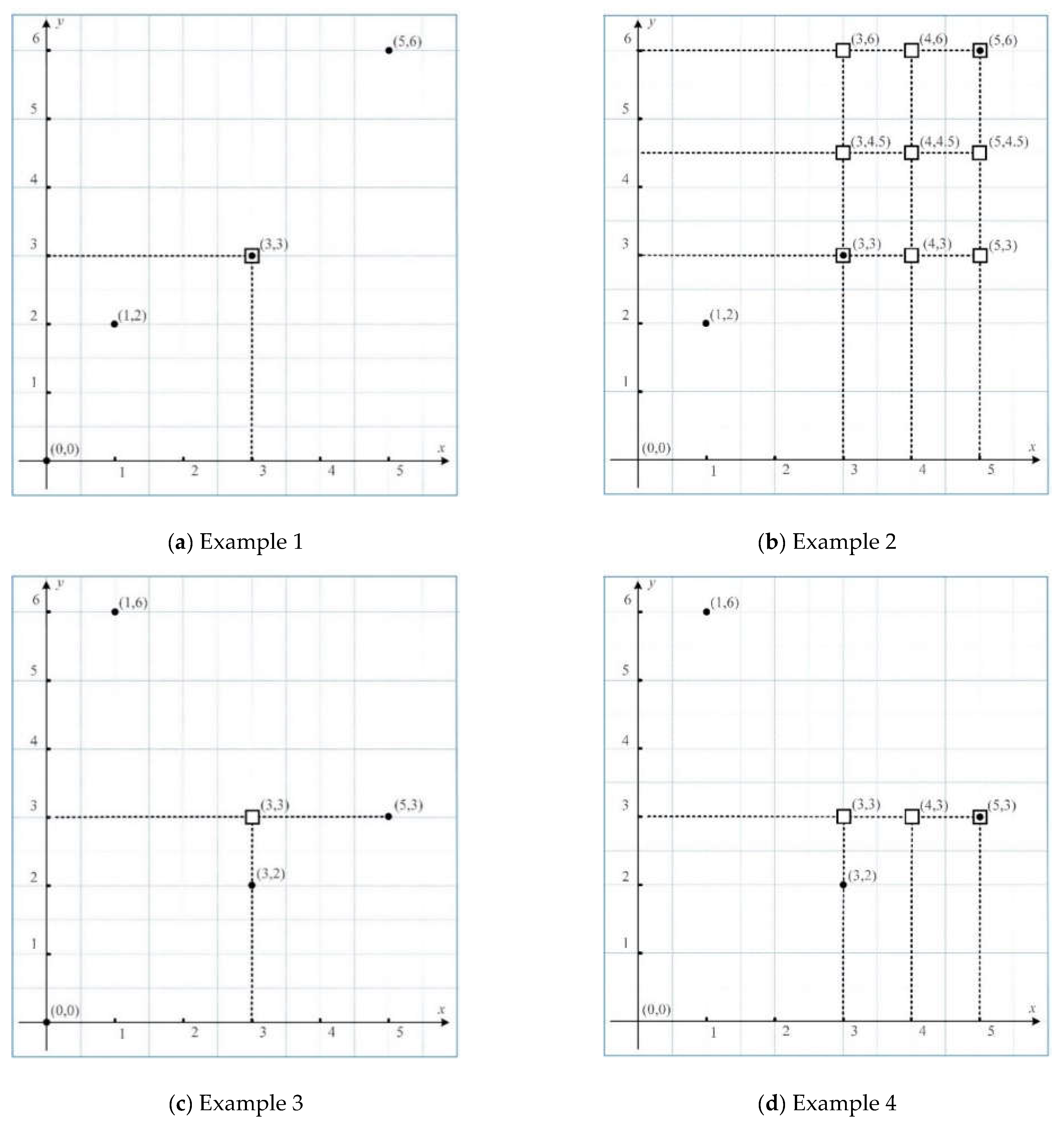Suppose that we choose only one minimizer among $x_{\left(k\right)}$, $x_{\left(k+1\right)}$, ($x_{\left(k\right)}+x_{\left(k+1\right)}$)/2 for the second case, we can construct the candidate facility locations. To better observe the characteristic of the optimal single-facility location, we use four examples (i.e., Examples 1–4) to illustrate the property of the optimal facility location, and the datasets are provided in

Table 2. Summary of data in four examples.

ID	Example 1			Example 2			Example 3			Example 4
	${\mathit{x}}_{\mathit{i}}$	${\mathit{y}}_{\mathit{i}}$	${\mathit{\omega }}_{\mathit{i}}$	${\mathit{x}}_{\mathit{i}}$	${\mathit{y}}_{\mathit{i}}$	${\mathit{\omega }}_{\mathit{i}}$	${\mathit{x}}_{\mathit{i}}$	${\mathit{y}}_{\mathit{i}}$	${\mathit{\omega }}_{\mathit{i}}$	${\mathit{x}}_{\mathit{i}}$	${\mathit{y}}_{\mathit{i}}$	${\mathit{\omega }}_{\mathit{i}}$
$i$ = 1	1	2	0.1	1	2	0.1	1	6	0.1	1	6	0.1
$i$ = 2	3	3	0.5	3	3	0.4	3	2	0.5	3	2	0.4
$i$ = 3	5	6	0.4	5	6	0.5	5	3	0.4	5	3	0.5

.

3.3.1. Example 1

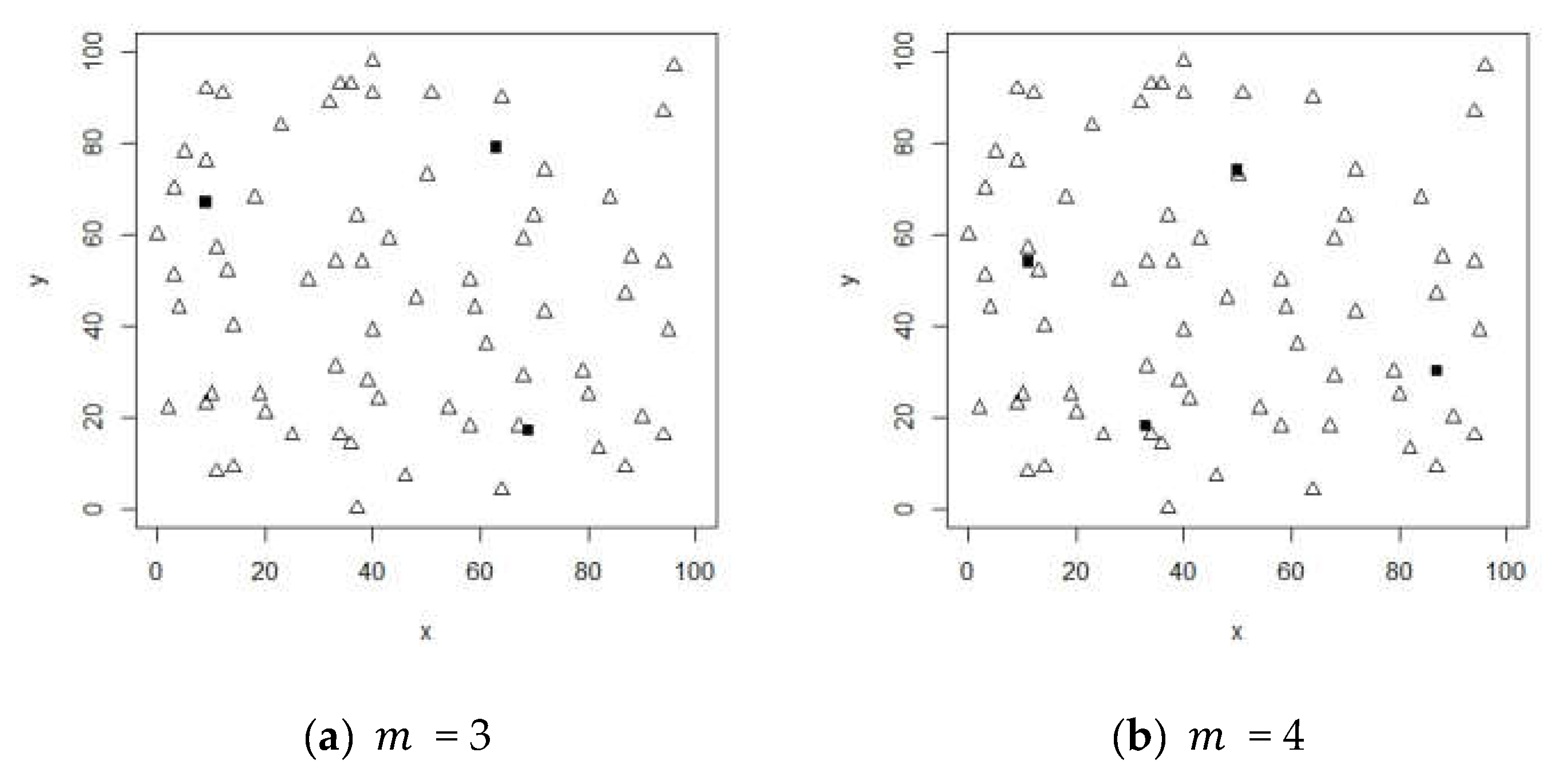
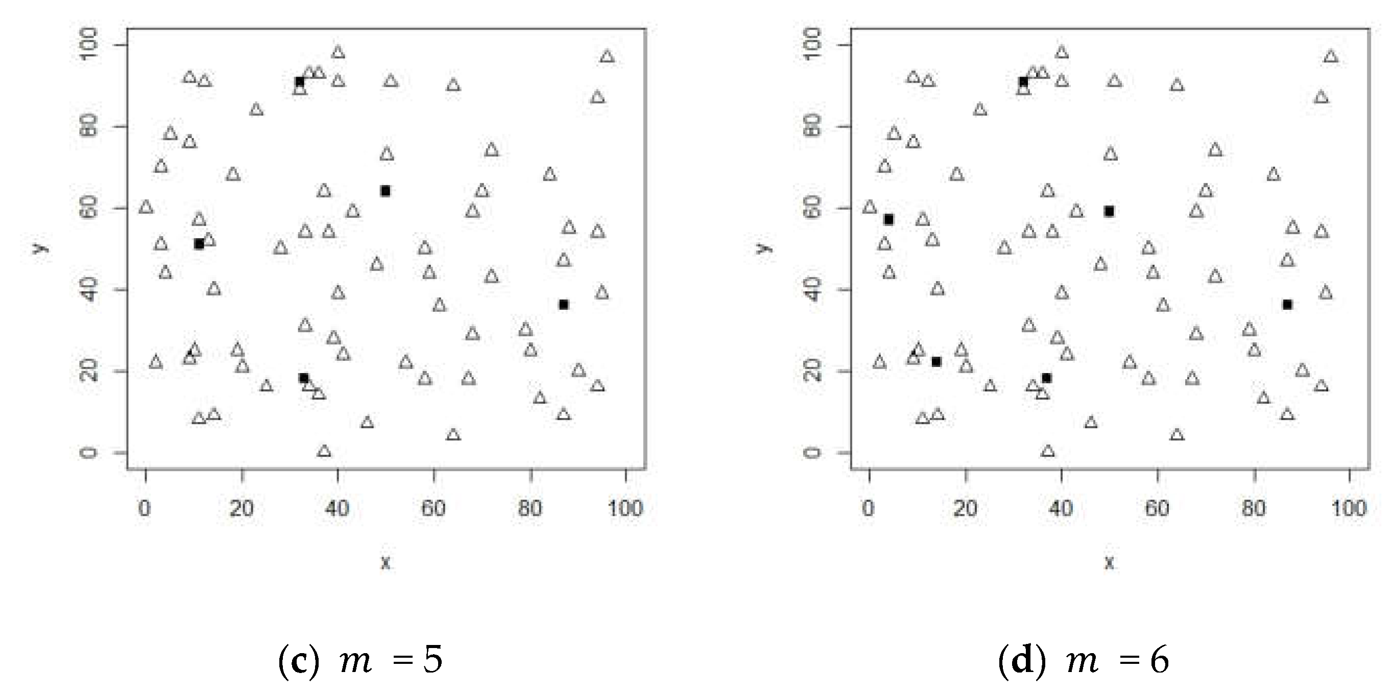
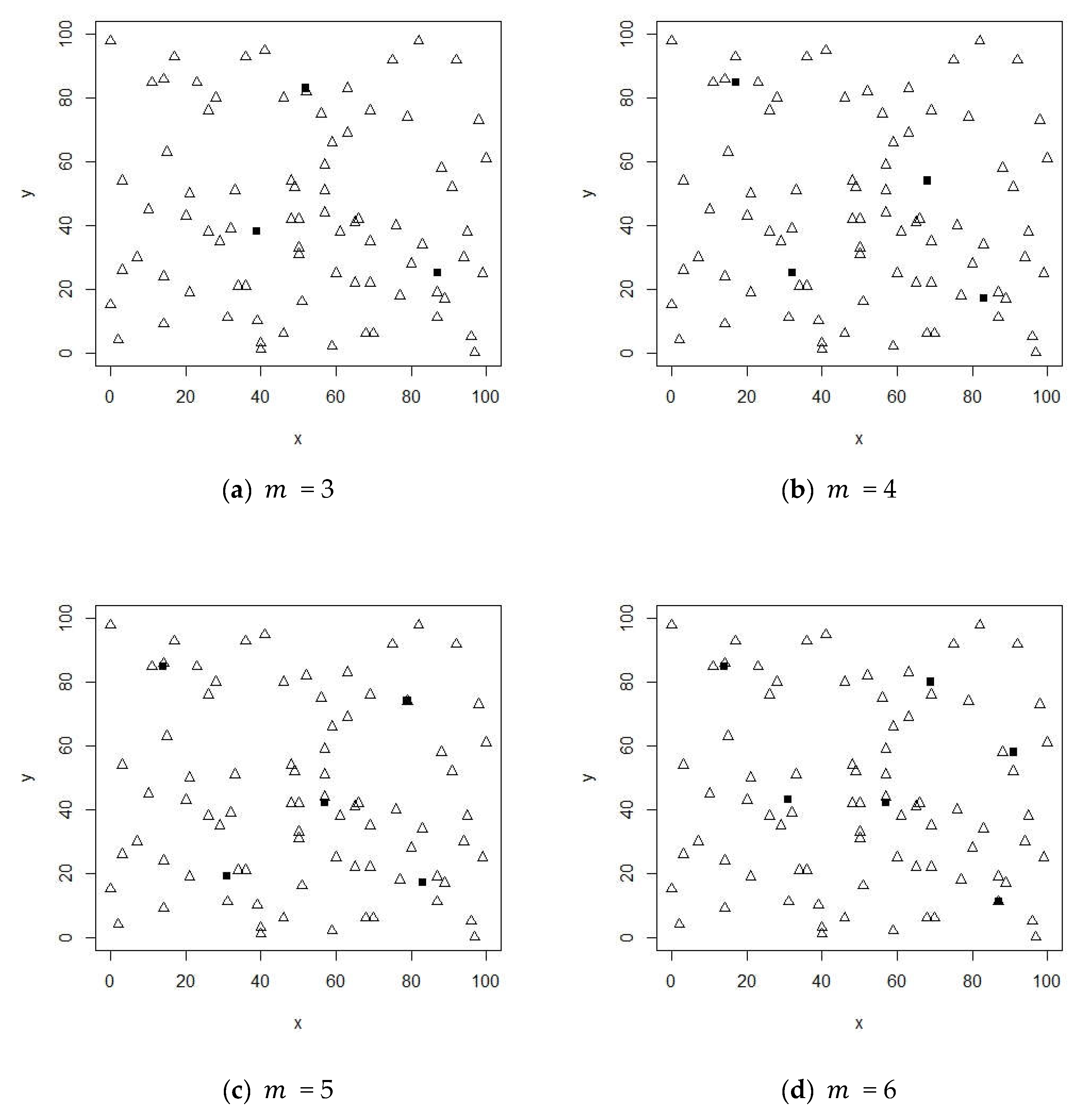
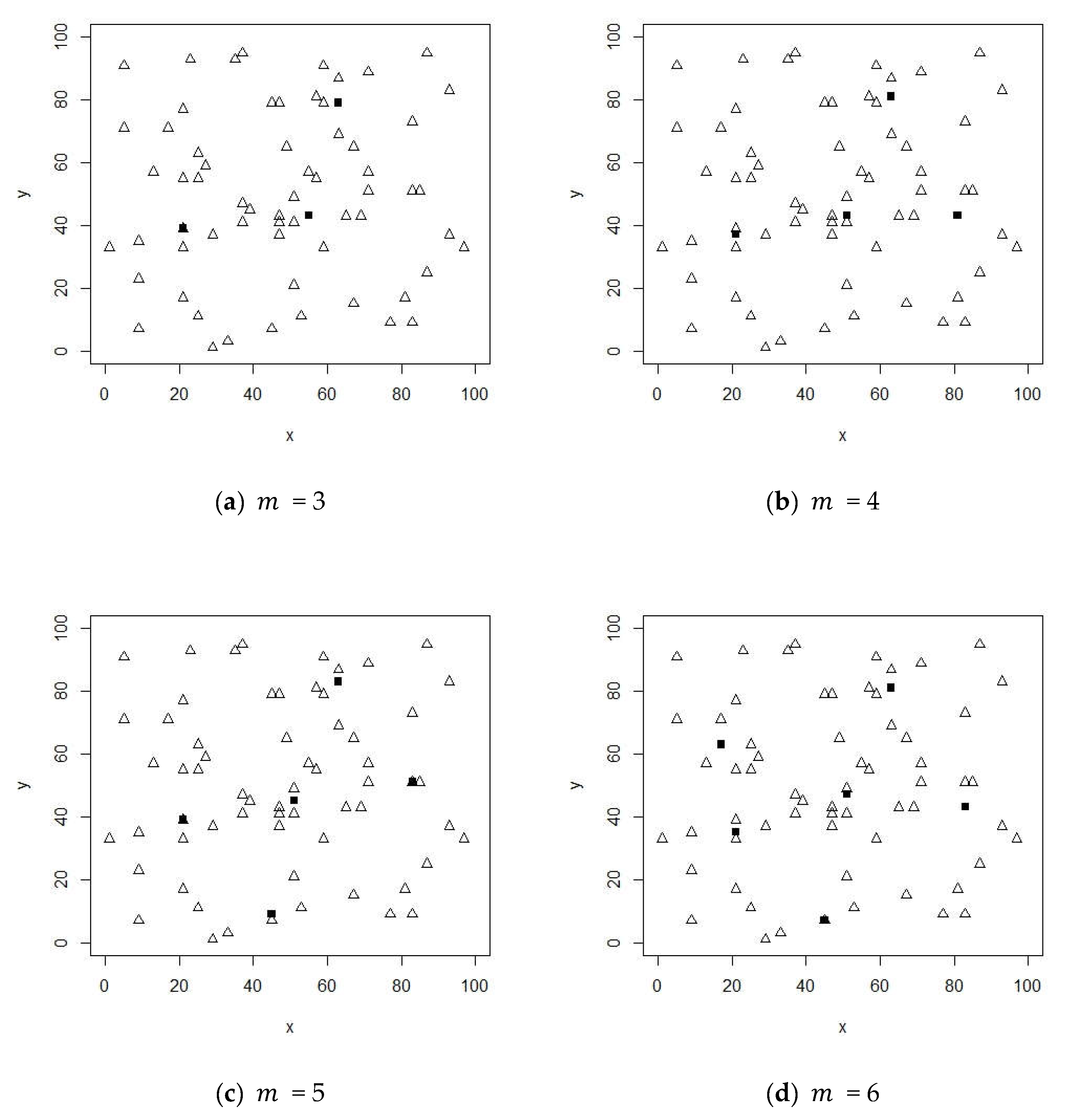
As shown in Figure 1, the black circles stand for the demand points and black hollow squares represent the optimal facility locations. In Example 1 (see Figure 1a), the optimal facility location is located at the second demand point due to its coordinate values and weights, which are given by

$$\tilde{u}= \mathrm{weighted} \mathrm{median} (x_1, x_2, x_3)=3$$

(25)

$$\tilde{v}= \mathrm{weighted} \mathrm{median} (y_1, y_2, y_3)=3$$

(26)

3.3.2. Example 2

There are four optimal facility locations (black hollow squares) in Example 2 (see Figure 1b) because of weight construction. Then, the weighted medians are given by

$$\tilde{u}= \mathrm{weighted} \mathrm{median} (x_1, x_2, x_3)=3, 5, \mathrm{or} 4$$

(27)

$$\tilde{v}= \mathrm{weighted} \mathrm{median} (y_1, y_2, y_3)=3, 6, \mathrm{or} 4.5$$

(28)

It is easy to obtain the optimal facility locations through permutation and combination of the weighted medians on different axes, which are (3, 3), (3, 6), (3, 4.5), (5, 3), (5, 6), (5, 4.5), (4, 3), (4, 6), and (4, 4.5). It is obvious that two of them, i.e., (3, 3) and (5, 6), are located at the demand points, but the others are not. As they have the same objective function value, any one among them can be considered as the location for the facility.

3.3.3. Example 3

As shown in Figure 1c, there is only one specific location for the facility due to the singular weighted median on each of the axis. The optimal facility location does not locate at the demand point, which is given by

$$\tilde{u}= \mathrm{weighted} \mathrm{median} (x_1, x_2, x_3)=3$$

(29)

$$\tilde{v}= \mathrm{weighted} \mathrm{median} (y_1, y_2, y_3)=3$$

(30)

3.3.4. Example 4

In this case, the weighted median on the axes are given by

$$\tilde{u}= \mathrm{weighted} \mathrm{median} (x_1, x_2, x_3)=3, 5, \mathrm{or} 4$$

(31)

$$\tilde{v}= \mathrm{weighted} \mathrm{median} (y_1, y_2, y_3)=3$$

(32)

Thus, there are three black hollow squares in Figure 1d, where any of them can be considered as the optimal location for the facility.

As presented in Figure 1 for Examples 1–4, we can conclude that the globally optimal facility location is based on the coordinate values of the observations on different axes. After constructing the set of mesh points that are consist of the coordinate combinations, it is obvious that the optimal single-facility location is an element from the set of mesh points. Then, we have the following formula

$$\left(\tilde{u},\tilde{v}\right)\in \left\{\left(x_i,y_j\right):i,j=1,2,\dots ,n\right\}\cup \left\{\left(\frac{x_i+x_{i+1}}{2},\frac{y_j+y_{j+1}}{2}\right):i,j=1,2,\dots ,n-1\right\}$$

(33)

Similarly, if we choose only one minimizer among $x_{\left(k\right)}$ and $x_{\left(k+1\right)}$ for the second case in (39), the optimal single-facility location is also an element from the other set of mesh points, which is given by

$$\left(\tilde{u},\tilde{v}\right)\in \left\{\left(x_i,y_j\right):i,j=1,2,\dots ,n\right\}$$

(34)

Note that the number of candidate locations in (34) is smaller than that in (33) but the objective function obtained through (34) is the same as that through (33). In this sense, the number of candidate locations in (34) is suggested in this study.

3.4. Identification of the Candidate Locations

As presented in (33), the globally optimal single-facility location is an element from the set of mesh points. Then, we investigate the candidate locations for the multi-facility location problem. In the multi-facility location problem, each demand point is assigned to its closest facility. Suppose that we have obtained the optimal facility locations, then the set of demand points served by the same facility is considered as a group, which is independent of other groups. In this sense, the optimal facility location is still one of the mesh points within this group. After considering the optimal facility locations for all groups, these optimal facility locations are from the mesh points that are constructed based on the observation coordinates. Then, we have

$$\left({\tilde{u}}_l,{\tilde{v}}_l\right)\in \left\{\left(x_i,y_j\right):i,j=1,2,\dots ,n\right\}\cup \left\{\left(\frac{x_i+x_{i+1}}{2},\frac{y_j+y_{j+1}}{2}\right):i,j=1,2,\dots ,n-1\right\} l=1, 2,\dots ,m$$

(35)

where $m$ is the number of facilities, which is indexed by $l$.

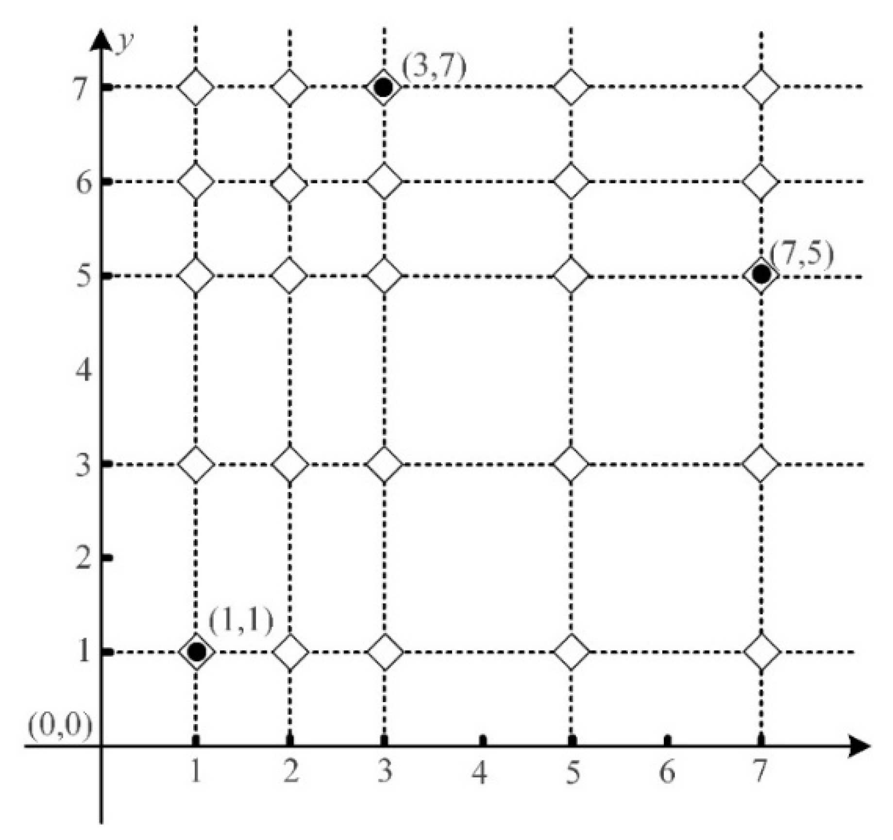
As an illustration, we provide an example to show the candidate locations (i.e., mesh points) for the facilities. In the example, we consider three demand points (see

Table 3. Data for the example with three demand points.

$\mathit{i}$	${\mathit{x}}_{\mathit{i}}$	${\mathit{y}}_{\mathit{i}}$	${\mathit{\omega }}_{\mathit{i}}$
1	1	1	0.3
2	3	7	0.2
3	7	5	0.5

). As shown in Figure 2, we construct the mesh points based on these three demand-point coordinates. Accordingly, 25 mesh points are represented by black hollow rhombuses that also contain three demand points. These 25 mesh points are considered as the candidate facility locations. It is easy to conclude that the number of candidate facilities $\mathrm{E}$ is related to the number of demand points$n$, where the relationship between them is given by

$$\mathrm{E}={\left(n+n-1\right)}^2=5^2=25$$

(36)

When the demand points have the same coordinate value on one axis, the number of candidate facilities $\mathrm{E}$ can be smaller. Suppose that there are $p$ ($p\le 2n-1$) different $x$-axis values and $q$ ($q\le 2n-1$) different $y$-axis values, the number of candidate facilities $\mathrm{E}$ can be smaller, which is given by

$$\mathrm{E} =pq\le {\left(2n-1\right)}^2$$

(37)

Based on the conclusion about the number of the candidate locations for the two-dimensional multi-facility location problem, it is easy to deduce the number of candidate locations for the three-dimensional multi-facility location problem, which is given by

$$\mathrm{E}\le {\left(2n-1\right)}^3$$

(38)

If we consider the minimizer from $x_{\left(k\right)}$ and $x_{\left(k+1\right)}$ for the second case presented in (39), the number of mesh points can be reduced and the number of candidate facilities $\mathrm{E}$ for the two- and three-dimensional multi-facility location problems are given below

$$\mathrm{E}\le {\left(n-1\right)}^2$$

(39)

$$\mathrm{E}\le {\left(n-1\right)}^3$$

(40)

Finally, we construct the candidate facility locations and transfer the continuous-space multi-facility location problem to the discrete-space multi-facility location problem. Next, our goal is to select the optimal locations from the mesh points, which is the global optimum solution to the problem.

3.5. Determination of the Globally Optimal Facility Locations

After the construction of the candidate locations for the facilities, what we need to do is to select the optimal facility locations from the mesh points. We formulate the mathematical model for the multi-facility location problem, which is also called the location-allocation problem. Besides, the construction of the candidate locations for the facilities makes it possible to determine the globally optimal locations for the capacitated facilities. Then, we present the different models for different facility location problems.

3.5.1. Model for the Uncapacitated Multi-Facility Problem

With the number of demand points $n$, we have $E$ candidate facility locations. Let $I$ be the set of demand points, which is indexed by $i$ with $i\in I$. Let $L$ be the set of candidate facility locations, which is indexed by $l$ with$l\in L$. Then, the distance from the candidate facility location $l$ to the demand point $i$ is known, which is denoted by $D_{li}$. Given the number of facilities$m>1$, our goal is to select $m$ locations among $\mathrm{E}$ candidate facility locations and allocate the demand points to these facilities to minimize the total cost. To formulate this problem, we need to define two more decision variables, which are given by

$$\begin{array}{ll}{g}_l& \{\begin{array}{cc}1& \mathrm{if} \mathrm{candidate} \mathrm{facility} l \mathrm{is} \mathrm{selected} \\ 0& \mathrm{otherwise} \end{array}\\ t_{il}& \{\begin{array}{cc}1& \mathrm{if} \mathrm{demand} \mathrm{point} i \mathrm{assigned} \mathrm{to} \mathrm{candidate} \mathrm{facility} l\\ 0& \mathrm{otherwise} \end{array}\end{array}$$

Then, we have the following mathematical model $ℳ1$ for the general multi-facility location-allocation problem:

• $ℳ1:$

$${\mathrm{Min} \mathrm{Obj}}_1=c{\sum }_{l=1}^{\mathrm{E}}{\sum }_{i=1}^n{\omega }_i{D}_{li}{t}_{il}$$

(41)

subject to

$${\sum }_{l=1}^{\mathrm{E}}{g}_l=m$$

(42)

$${\sum }_{l=1}^{\mathrm{E}}{t}_{il}=1 \forall i\in I$$

(43)

$$t_{il}\le g_l \forall i\in I \mathrm{and} \forall l\in L$$

(44)

The objective function in (41) minimizes the total weighted travel cost. Constraint in (42) means that we must locate exactly $m$ facilities. Constraint (43) states that a demand point can only be serviced by one facility. Constraint (44) indicates that the demand point can only be assigned to the opened facility.

3.5.2. Model for the Uncapacitated Multi-Facility Problem with Fixed Cost

In the above mathematical model, the fixed cost of opening a facility is not considered. However, in practice, the fixed cost of opening a facility is inevitable. Thus, the fixed cost, denoted by $F$, needs to be considered in the multi-facility location-allocation problem. In this sense, the number of facilities is also a decision variable. Then, the mathematical model $ℳ2$ is given by

• $ℳ2:$

$${\mathrm{Min} \mathrm{Obj}}_2=c{\sum }_{l=1}^{\mathrm{E}}{\sum }_{i=1}^n{\omega }_i{D}_{li}{t}_{il}+\mathrm{F}{\sum }_{l=1}^{\mathrm{E}}{g}_l$$

(45)

subject to

$${\sum }_{l=1}^{\mathrm{E}}{g}_l\le n$$

(46)

$${\sum }_{l=1}^{\mathrm{E}}{t}_{il}=1 \forall i\in I$$

(47)

$$t_{il}\le g_l \forall i\in I \mathrm{and} \forall l\in L$$

(48)

The objective function in (45) minimizes the total cost including the weighted travel cost and fixed cost. The first constraint in (46) means that the number of facilities cannot be more than $n$. Constraints (47) and (48) are the same as the Constraints (43) and (44).

3.5.3. Model for the Capacitated Multi-Facility Problem with Fixed Cost

Generally, the clustering-based method is applied to solve the uncapacitated continuous-space multi-facility location problem. Even though some studies have applied the adjusted clustering-based algorithms to solve the capacitated multi-facility problem [30,31], it is still impossible to guarantee the global optimum of the solution. In this sense, obtaining the globally optimal locations for the facilities is warranted when the practical factor of the limited capacities is considered. Based on the constructed candidate locations for the facilities, the globally optimal locations for the capacitated facilities also can be selected from the mesh points. Let $r_i$ be the quantity of demand at demand point $i$ and $Ca{p}_l$ be the capacity of the facility $l$. Note that $r_i$ can be considered as the weight of demand point $i$. Then, the capacitated continuous-space multi-facility problem can be formulated as the following mathematical model $ℳ3$.

• $ℳ3:$

$${\mathrm{Min} \mathrm{Obj}}_3=c{\sum }_{l=1}^{\mathrm{E}}{\sum }_{i=1}^n{r}_i{D}_{li}{t}_{il}+\mathrm{F}{\sum }_{l=1}^{\mathrm{E}}{g}_l$$

(49)

subject to

$${\sum }_{l=1}^{\mathrm{E}}{g}_l\le n$$

(50)

$${\sum }_{l=1}^{\mathrm{E}}{t}_{il}=1 \forall i\in I$$

(51)

$$t_{il}\le g_l \forall i\in I, l\in L$$

(52)

$${\sum }_{i=1}^n{r}_i{t}_{il}\le Ca{p}_l \forall l\in L$$

(53)

The objective function in (49) minimizes the total cost including the travel cost and fixed cost. The first constraint in (50) guarantees the maximum number of facilities. Constraints (51) and (52) are the same as the Constraints (43) and (44). Constraint (53) restricts the facility capacity.

4. Numerical Examples

In this section, several illustrative instances from a benchmark composed of 27 instances (http://neo.lcc.uma.es/vrp/, accessed on 1 May 2020) referred to Augerat, Belenguer [64] are provided to evaluate the performance of the proposed method. Each instance provides customers’ (demand point) geographical coordinates and quantities of demand. The proposed exact approach is used to determine the globally optimal facility locations under different numbers of facilities for four instances (see

Table 4. Summary of the benchmark Instances 24–27.

No.	1	2	3	4
Instance ID	24	25	26	27
Problem size	64	65	69	80

) from the benchmark (i.e., Instances 24–27).

Given the parameter values, the proposed models (i.e., $ℳ1$,$ℳ2$,$ℳ3$) are implemented in the IBM ILOG CPLEX Optimization Studio (Version: 12.6). All the experiments are run on a computer with an Intel(R) Core(TM) i7-7700 [email protected] GHz and 8 GB memory under the Windows 10 Pro system. In what follows, the numerical results are provided to validate the effectiveness of the proposed method. Then, the proposed method is compared with the previous clustering-based methods, where the comparison results are also provided to illustrate the advantages of the proposed method.

4.1. Numerical Results

First of all, the model $ℳ1$ is applied and the facility locations are presented in Figure 3, Figure 4, Figure 5 and Figure 6 for Instances 24–27. As shown in Figure 3, Figure 4, Figure 5 and Figure 6, different numbers of the facilities (i.e., 3, 4, 5, and 6) are tested for each of the instances, where the black hollow triangle stands for the demand point and the solid square is represented as the facility. It is obvious that the facility locations are well scattered in the planning area. Since the difference between the models $ℳ1$ and $ℳ2$ is subject to whether the fixed cost is considered, the same results but with different objective function values are obtained based on the models $ℳ1$ and $ℳ2$.

Similarly, the globally optimal facility locations can also be obtained when the facility capacities are considered in model $ℳ3$. As shown in Figure 7, the facility locations are determined for Instance 24 when different numbers of facilities are considered, which verifies the effectiveness of the proposed approach in obtaining the globally optimal facility locations, even though the facility capacities are involved. Note that similar results can be obtained when Instances 25–27 are considered. It is also obvious that the globally optimal facility locations obtained from model $ℳ3$ are different from those in models $ℳ1$ and $ℳ2$, which indicates that the facility capacities have a great influence on the multi-facility location determination problem.

Next, the influence of different numbers of facilities and fixed costs on the objective function values are tested for models $ℳ1$, $ℳ2$, and $ℳ3$. Regarding model $ℳ1$, the objective function value is only affected by the number of facilities. In this sense, the relationship between the number of facilities and the objective function value is presented in Figure 8 given different shipping costs. It is obvious that the increase in the number of facilities always decreases the total cost, no matter how the shipping cost changes.

When the fixed cost is considered at facilities, in addition to the number of facilities, the fixed cost also has a great influence on the objective function value. To further provide a visual illustration of the influence of the parameters$m$ and $\mathrm{F}$ on the total cost, a cross-validation experiment is carried out when the number of facilities $m$ goes from 2 to 18 and fixed cost $\mathrm{F}$ goes from 60 to 360. Then, the results under different shipping costs are presented in Figure 9, Figure 10, Figure 11, Figure 12 and Figure 13. Specifically, as shown in Figure 9, the growth in the fixed cost from 60 to 360 increases the total cost. However, when the number of facilities $m$ goes from 2 to 18, the total cost decreases first, since more facilities lead to lower transportation costs, and then the total cost increases because too many facilities contribute to marginally lower transportation costs, but result in higher fixed costs. Similar results are obtained in Figure 10, Figure 11, Figure 12 and Figure 13. As a consequence, an appropriate number of facilities needs to be determined so that the globally minimum total cost can be obtained.

To investigate the influence of the capacitated facilities on the optimal facility locations and objective function values, the proposed three models $ℳ1$, $ℳ2$, and $ℳ3$ are compared in terms of Instance 24 and the corresponding comparison results are provided in

Table 5. Comparison of optimal solutions and objective function values among three models.

Number of Facilities	ID	$\mathit{ℳ}1$		$\mathit{ℳ}2$		$\mathit{ℳ}3$
		Facility Locations	$\mathbf{O}\mathbf{b}\mathbf{j}1$	Facility Locations	$\mathbf{O}\mathbf{b}\mathbf{j}2$	Facility Capacities	Facility Locations	$\mathbf{O}\mathbf{b}\mathbf{j}3$
3	1	(55, 43)	2932	(55, 43)	3292	350	(49, 43)	3332
	2	(21, 39)		(21, 39)			(63, 79)
	3	(63, 81)		(63, 81)			(21, 39)
4	1	(21, 37)	2480	(21, 37)	2960	250	(21, 37)	2993
	2	(51, 43)		(51, 43)			(51, 43)
	3	(63, 83)		(63, 83)			(81, 43)
	4	(83, 51)		(83, 51)			(63, 81)
5	1	(51, 43)	2156	(51, 43)	2756	220	(45, 9)	2774
	2	(45, 9)		(45, 9)			(21, 39)
	3	(83, 51)		(83, 51)			(83, 51)
	4	(59, 83)		(59, 83)			(63, 83)
	5	(21, 39)		(21, 39)			(51, 45)
6	1	(51, 43)	1872	(51, 43)	2592	150	(45, 7)	2635
	2	(51, 9)		(51, 9)			(83, 43)
	3	(17, 63)		(17, 63)			(17, 63)
	4	(63, 81)		(63, 81)			(21, 35)
	5	(21, 33)		(21, 33)			(63, 81)
	6	(83, 51)		(83, 51)			(51, 47)

. Regarding the models $ℳ1$ and $ℳ2$, the same facility locations are obtained because the fixed cost does not influence the determination of the facility locations. When the facility capacities are considered, the globally optimal facility locations in model $ℳ3$ can still be obtained, which is different from that in model $ℳ2$. Besides, a higher total cost is obtained in model $ℳ3$ compared with model $ℳ2$, which verifies that the facility capacities affect the determination of facility locations.

4.2. Comparison with Previous Methods

When the potential facility candidates are not given, the general strategy to determine the set of facility locations is the application of clustering-based algorithms. Among them, the K-means clustering algorithm is one of the most popular methods in handling continuous multi-facility location problems. However, the minimizer of the total weighted Manhattan distance is the weighted median rather than the weighted mean in each cluster. In this sense, the weighted median is used to update the cluster center in each of the iterations in the clustering-based algorithms [18]. In addition, Gao, Nayeem [40] also developed a clustering-based genetic algorithm for the continuous multi-facility location problem considering the Manhattan distance.

To illustrate the outperformance of the proposed approach, different methods are compared for Instances 24–27 in handling the continuous multi-facility location problems. Given different numbers of facilities, the comparison results including objective function values and the facility locations are presented in Figure 13 and Table 6, Table 7, Table 8 and Table 9, respectively. Since different randomly generated initial solutions result in different clustering results, we repeat each simulation five times and pick up the best one among them. As shown in Figure 13, the performance of minimizing the total transportation cost using different methods is presented. The proposed method outperforms other clustering-based algorithms. Besides, given any number of facilities from 2 to 12, the method proposed by Gao [65] demonstrates better performance in reducing the total transportation cost compared with the k-means method and clustering-based genetic algorithm, since the weighted median is used to update the cluster center. Besides, from Table 6, Table 7, Table 8 and Table 9, the facility locations obtained using the method proposed by Gao [65] are closer to the globally optimal solution compared with the other two existing methods. In this sense, the method proposed by Gao [65] is more appropriate to determine the optimal solution when the problem size is quite large. As a consequence, regarding the Manhattan distance, there is definitely strong evidence that the proposed exact method can determine the globally optimal facility locations for the continuous multi-facility location problems. Moreover, the application of the weighted median in the clustering-based methods is also reasonable when the Manhattan distance is considered.

Table 6. Comparison of facility locations using different methods for Instance 24.

Number of Facilities	ID	K-Means Clustering Algorithm	Gao, Nayeem [40]	Gao [65]	The Proposed Method
3	1	(51.7, 13.0)	(20.6, 42.6)	(55, 43)	(55, 43)
	2	(30.6, 48.6)	(68.3, 74.4)	(21, 39)	(21, 39)
	3	(69.5, 66.1)	(58.8, 35.8)	(63, 79)	(63, 81)
4	1	(56.9, 13.4)	(30.3, 73.3)	(21, 37)	(21, 37)
	2	(73.7, 66.1)	(71.3, 79.0)	(51, 43)	(51, 43)
	3	(16.2, 43.1)	(60.1, 38.2)	(63, 81)	(63, 83)
	4	(44.7, 54.5)	(17.7, 33.0)	(83, 43)	(83, 51)
5	1	(36.9, 8.8)	(19.6, 65.6)	(51, 49)	(51, 43)
	2	(18.0, 48.6)	(18.5, 27.8)	(51, 9)	(45, 9)
	3	(75.7, 38.0)	(66.6, 81.2)	(71, 43)	(83, 51)
	4	(48.6, 47.5)	(77.4, 38.5)	(63, 81)	(59, 83)
	5	(48.6, 47.5)	(49.2, 39.7)	(21, 39)	(21, 39)
6	1	(62.6, 84.5)	(47.2, 45.7)	(51, 47)	(51, 43)
	2	(83.5, 20.2)	(63.9, 52.2)	(45, 7)	(51, 9)
	3	(17.9, 47.7)	(86.6, 45.0)	(17, 63)	(17, 63)
	4	(35.3, 7.5)	(17.5, 44.8)	(63, 81)	(63, 81)
	5	(50.0, 43.4)	(55.1, 9.5)	(21, 35)	(21, 33)
	6	(71.8, 55.6)	(64.9, 85.0)	(83, 15)	(83, 51)

Table 6. Comparison of facility locations using different methods for Instance 24.

Number of Facilities	ID	K-Means Clustering Algorithm	Gao, Nayeem [40]	Gao [65]	The Proposed Method
3	1	(51.7, 13.0)	(20.6, 42.6)	(55, 43)	(55, 43)
	2	(30.6, 48.6)	(68.3, 74.4)	(21, 39)	(21, 39)
	3	(69.5, 66.1)	(58.8, 35.8)	(63, 79)	(63, 81)
4	1	(56.9, 13.4)	(30.3, 73.3)	(21, 37)	(21, 37)
	2	(73.7, 66.1)	(71.3, 79.0)	(51, 43)	(51, 43)
	3	(16.2, 43.1)	(60.1, 38.2)	(63, 81)	(63, 83)
	4	(44.7, 54.5)	(17.7, 33.0)	(83, 43)	(83, 51)
5	1	(36.9, 8.8)	(19.6, 65.6)	(51, 49)	(51, 43)
	2	(18.0, 48.6)	(18.5, 27.8)	(51, 9)	(45, 9)
	3	(75.7, 38.0)	(66.6, 81.2)	(71, 43)	(83, 51)
	4	(48.6, 47.5)	(77.4, 38.5)	(63, 81)	(59, 83)
	5	(48.6, 47.5)	(49.2, 39.7)	(21, 39)	(21, 39)
6	1	(62.6, 84.5)	(47.2, 45.7)	(51, 47)	(51, 43)
	2	(83.5, 20.2)	(63.9, 52.2)	(45, 7)	(51, 9)
	3	(17.9, 47.7)	(86.6, 45.0)	(17, 63)	(17, 63)
	4	(35.3, 7.5)	(17.5, 44.8)	(63, 81)	(63, 81)
	5	(50.0, 43.4)	(55.1, 9.5)	(21, 35)	(21, 33)
	6	(71.8, 55.6)	(64.9, 85.0)	(83, 15)	(83, 51)

Table 7. Comparison of facility locations using different methods for Instance 25.

Number of Facilities	ID	K-Means Clustering Algorithm	Gao, Nayeem [40]	Gao [65]	The Proposed Method
3	1	(31.9, 77.1)	(74.5, 21.8)	(15, 69)	(39, 67)
	2	(81.0, 32.1)	(40.1, 76.9)	(75, 75)	(63, 79)
	3	(30.0, 19.5)	(23.6, 19.0)	(49, 19)	(69, 17)
4	1	(70.5, 77.8)	(16.1, 74.5)	(25, 19)	(25, 19)
	2	(16.1, 74.5)	(69.5, 80.2)	(15, 69)	(15, 69)
	3	(24.3, 17.0)	(47.8, 17.5)	(63, 77)	(63, 77)
	4	(74.1, 21.2)	(90.6, 40.9)	(77, 17)	(77, 17)
5	1	(26.8, 18.4)	(14.8, 21.1)	(77, 17)	(75, 17)
	2	(27.2, 83.6)	(49.7, 17.7)	(63, 77)	(63, 77)
	3	(76.2, 20.3)	(71.4, 78.9)	(15, 69)	(15, 69)
	4	(70.5, 77.8)	(80.0, 22.2)	(47, 21)	(91, 41)
	5	(7.1, 67.0)	(16.3, 75.2)	(15, 19)	(25, 19)
6	1	(15.1, 19.8)	(89.4, 36.3)	(15, 69)	(15, 69)
	2	(7.1, 67.0)	(71.5, 14.7)	(47, 21)	(47, 21)
	3	(71.4, 78.9)	(16.1, 74.5)	(77, 17)	(77, 17)
	4	(78. 7, 20.1)	(89.6, 72.5)	(63, 77)	(77, 77)
	5	(27.2, 83.6)	(26.8, 18.4)	(93, 41)	(15, 41)
	6	(46.7, 20.5)	(61.2, 80.4)	(9, 19)	(25, 19)

Table 7. Comparison of facility locations using different methods for Instance 25.

Number of Facilities	ID	K-Means Clustering Algorithm	Gao, Nayeem [40]	Gao [65]	The Proposed Method
3	1	(31.9, 77.1)	(74.5, 21.8)	(15, 69)	(39, 67)
	2	(81.0, 32.1)	(40.1, 76.9)	(75, 75)	(63, 79)
	3	(30.0, 19.5)	(23.6, 19.0)	(49, 19)	(69, 17)
4	1	(70.5, 77.8)	(16.1, 74.5)	(25, 19)	(25, 19)
	2	(16.1, 74.5)	(69.5, 80.2)	(15, 69)	(15, 69)
	3	(24.3, 17.0)	(47.8, 17.5)	(63, 77)	(63, 77)
	4	(74.1, 21.2)	(90.6, 40.9)	(77, 17)	(77, 17)
5	1	(26.8, 18.4)	(14.8, 21.1)	(77, 17)	(75, 17)
	2	(27.2, 83.6)	(49.7, 17.7)	(63, 77)	(63, 77)
	3	(76.2, 20.3)	(71.4, 78.9)	(15, 69)	(15, 69)
	4	(70.5, 77.8)	(80.0, 22.2)	(47, 21)	(91, 41)
	5	(7.1, 67.0)	(16.3, 75.2)	(15, 19)	(25, 19)
6	1	(15.1, 19.8)	(89.4, 36.3)	(15, 69)	(15, 69)
	2	(7.1, 67.0)	(71.5, 14.7)	(47, 21)	(47, 21)
	3	(71.4, 78.9)	(16.1, 74.5)	(77, 17)	(77, 17)
	4	(78. 7, 20.1)	(89.6, 72.5)	(63, 77)	(77, 77)
	5	(27.2, 83.6)	(26.8, 18.4)	(93, 41)	(15, 41)
	6	(46.7, 20.5)	(61.2, 80.4)	(9, 19)	(25, 19)

Table 8. Comparison of facility locations using different methods for Instance 26.

Number of Facilities	ID	K-Means Clustering Algorithm	Gao, Nayeem [40]	Gao [65]	The Proposed Method
3	1	(78.2, 39.2)	(24.1, 22.5)	(38, 73)	(9, 67)
	2	(20.7, 25.5)	(26.9, 72.0)	(14, 25)	(63, 79)
	3	(29.4, 74.4)	(79.3, 40.3)	(87, 29)	(69, 17)
4	1	(20.8, 71.1)	(47.3, 70.6)	(40, 89)	(50, 74)
	2	(61.8, 70.2)	(27.1, 18.6)	(11, 54)	(11, 54)
	3	(22.5, 22.7)	(9.9, 62.1)	(33, 18)	(33, 18)
	4	(81.5, 29.6)	(83.9, 35.0)	(80, 39)	(87, 30)
5	1	(84.4, 32.0)	(41.2, 70.6)	(87, 36)	(87, 36)
	2	(26.1, 76.1)	(83.9, 58.4)	(33, 18)	(33, 18)
	3	(9.0, 34.7)	(23.3, 17.3)	(50, 64)	(50, 64)
	4	(64.8, 74.5)	(75.8, 21.7)	(4, 51)	(11, 51)
	5	(39.5, 21.3)	(9.1, 60.8)	(23, 91)	(32, 91)
6	1	(35.7, 84.8)	(46.0, 74.0)	(80, 18)	(87, 36)
	2	(29.0, 9.0)	(11.3, 64.6)	(88, 54)	(14, 22)
	3	(11.5, 54.3)	(21.1, 29.8)	(48, 54)	(50, 59)
	4	(84.3, 41.2)	(85.6, 56.2)	(32, 91)	(32, 91)
	5	(45.1, 37.6)	(75.8, 21.7)	(9, 51)	(4, 57)
	6	(11.1, 22.7)	(26.2, 9.3)	(25, 16)	(37, 18)

Table 8. Comparison of facility locations using different methods for Instance 26.

Number of Facilities	ID	K-Means Clustering Algorithm	Gao, Nayeem [40]	Gao [65]	The Proposed Method
3	1	(78.2, 39.2)	(24.1, 22.5)	(38, 73)	(9, 67)
	2	(20.7, 25.5)	(26.9, 72.0)	(14, 25)	(63, 79)
	3	(29.4, 74.4)	(79.3, 40.3)	(87, 29)	(69, 17)
4	1	(20.8, 71.1)	(47.3, 70.6)	(40, 89)	(50, 74)
	2	(61.8, 70.2)	(27.1, 18.6)	(11, 54)	(11, 54)
	3	(22.5, 22.7)	(9.9, 62.1)	(33, 18)	(33, 18)
	4	(81.5, 29.6)	(83.9, 35.0)	(80, 39)	(87, 30)
5	1	(84.4, 32.0)	(41.2, 70.6)	(87, 36)	(87, 36)
	2	(26.1, 76.1)	(83.9, 58.4)	(33, 18)	(33, 18)
	3	(9.0, 34.7)	(23.3, 17.3)	(50, 64)	(50, 64)
	4	(64.8, 74.5)	(75.8, 21.7)	(4, 51)	(11, 51)
	5	(39.5, 21.3)	(9.1, 60.8)	(23, 91)	(32, 91)
6	1	(35.7, 84.8)	(46.0, 74.0)	(80, 18)	(87, 36)
	2	(29.0, 9.0)	(11.3, 64.6)	(88, 54)	(14, 22)
	3	(11.5, 54.3)	(21.1, 29.8)	(48, 54)	(50, 59)
	4	(84.3, 41.2)	(85.6, 56.2)	(32, 91)	(32, 91)
	5	(45.1, 37.6)	(75.8, 21.7)	(9, 51)	(4, 57)
	6	(11.1, 22.7)	(26.2, 9.3)	(25, 16)	(37, 18)

Table 9. Comparison of facility locations using different methods for Instance 27.

Number of Facilities	ID	K-Means Clustering Algorithm	Gao, Nayeem [40]	Gao [65]	The Proposed Method
3	1	(83.4, 35.3)	(47.7, 77.0)	(88, 35)	(87, 25)
	2	(13.7, 63.7)	(79.7, 28.3)	(39, 22)	(39, 38)
	3	(48.9, 45.3)	(29.6, 28.5)	(49, 82)	(52, 83)
4	1	(70.4, 62.2)	(27.4, 27.3)	(14, 85)	(17, 85)
	2	(79.6, 19.4)	(37.4, 86.8)	(34, 26)	(32, 25)
	3	(23.0, 81.9)	(69.4, 53.5)	(83, 17)	(83, 17)
	4	(32.3, 25.9)	(80.5, 16.7)	(69, 58)	(68, 54)
5	1	(27.3, 22.3)	(79.6, 19.4)	(50, 42)	(57, 42)
	2	(80.6, 71.2)	(82.8, 70.9)	(14, 85)	(14, 85)
	3	(57.2, 44.0)	(53.9, 50.9)	(88, 30)	(83, 17)
	4	(81.6, 16.3)	(28.9, 20.1)	(39, 10)	(31, 19)
	5	(23.0, 82.1)	(19.0, 78.8)	(63, 76)	(79, 74)
6	1	(53.9, 45.9)	(16.1, 41.9)	(57, 42)	(57, 42)
	2	(80.6, 71.2)	(26.4, 87.0)	(69, 80)	(69, 80)
	3	(78.5, 28.5)	(57.8, 43.8)	(31, 19)	(31, 43)
	4	(22.3, 28.3)	(82.5, 16.9)	(80, 11)	(87, 11)
	5	(75.7, 5.1)	(80.6, 71.2)	(14, 85)	(14, 85)
	6	(26.2, 86.7)	(35.2, 11.7)	(91, 52)	(91, 58)

Table 9. Comparison of facility locations using different methods for Instance 27.

Number of Facilities	ID	K-Means Clustering Algorithm	Gao, Nayeem [40]	Gao [65]	The Proposed Method
3	1	(83.4, 35.3)	(47.7, 77.0)	(88, 35)	(87, 25)
	2	(13.7, 63.7)	(79.7, 28.3)	(39, 22)	(39, 38)
	3	(48.9, 45.3)	(29.6, 28.5)	(49, 82)	(52, 83)
4	1	(70.4, 62.2)	(27.4, 27.3)	(14, 85)	(17, 85)
	2	(79.6, 19.4)	(37.4, 86.8)	(34, 26)	(32, 25)
	3	(23.0, 81.9)	(69.4, 53.5)	(83, 17)	(83, 17)
	4	(32.3, 25.9)	(80.5, 16.7)	(69, 58)	(68, 54)
5	1	(27.3, 22.3)	(79.6, 19.4)	(50, 42)	(57, 42)
	2	(80.6, 71.2)	(82.8, 70.9)	(14, 85)	(14, 85)
	3	(57.2, 44.0)	(53.9, 50.9)	(88, 30)	(83, 17)
	4	(81.6, 16.3)	(28.9, 20.1)	(39, 10)	(31, 19)
	5	(23.0, 82.1)	(19.0, 78.8)	(63, 76)	(79, 74)
6	1	(53.9, 45.9)	(16.1, 41.9)	(57, 42)	(57, 42)
	2	(80.6, 71.2)	(26.4, 87.0)	(69, 80)	(69, 80)
	3	(78.5, 28.5)	(57.8, 43.8)	(31, 19)	(31, 43)
	4	(22.3, 28.3)	(82.5, 16.9)	(80, 11)	(87, 11)
	5	(75.7, 5.1)	(80.6, 71.2)	(14, 85)	(14, 85)
	6	(26.2, 86.7)	(35.2, 11.7)	(91, 52)	(91, 58)

5. Conclusions

This study focused on determining the globally optimal facility locations for continuous-space multi-facility location problems when the Manhattan distance is considered. Before the exact method was proposed, we started with the continuous-space single-facility location problem and found the global minimizer for the problem using a statistical approach. More specifically, in terms of Manhattan distance with weights, the weighted median is the global minimizer to the total weighted Manhattan distance. Thus, we investigated and defined the weighted median more clearly compared to the existing methods. Based on the newly observed properties from the weighted median, we extended it to high-dimension multi-facility problems and transferred the continuous-space location problem to the discrete-space location problem. As a consequence, three mathematical models were proposed to formulate different types of continuous-space multi-facility location problem and the corresponding globally optimal solutions are obtained, which is different from the previous clustering-based methods. To illustrate the effectiveness and efficiency of the proposed exact method, several illustrative instances from a benchmark were used to compare the performances of different methods. The comparison results show the superiority of the proposed exact method in the decision-making of the continuous-space multi-facility location problems.

Despite the above contributions and insights, this work still has several limitations. This study only investigated a continuous-space multi-facility location problem based on the Manhattan distance. Moreover, it is difficult to determine the global optimum when the problem size is quite large. Accordingly, some meaningful problems of interest can be explored in more depth in future. It is important to find the candidate locations of the facilities for the Euclidean distance. Besides, we also need to develop a heuristic algorithm to determine the facility locations based on all of the candidate locations when the problem size is large. Furthermore, the maximum distance (i.e., blast radius) from the facility to the demand point will be considered in the continuous-space multi-facility location problem.