Article

Early Neighbor Rejection-Aided Tabu Search Detection for Large MIMO Systems

Research and Development, TJ-INNOVATION, Jomaru-ro 385, Beon-gil, Bucheon-si 14557, Gyeonggi-do, Korea
*
Author to whom correspondence should be addressed.
Appl. Sci. 2021, 11(16), 7305; https://doi.org/10.3390/app11167305
Submission received: 20 June 2021 / Revised: 29 July 2021 / Accepted: 30 July 2021 / Published: 9 August 2021
(This article belongs to the Section Electrical, Electronics and Communications Engineering)

Abstract

:
In this study, a low complexity tabu search (TS) algorithm for multiple-input multiple-output (MIMO) systems is proposed. To reduce the computational complexity of the TS algorithm, early neighbor rejection (ENR) and layer ordering schemes are employed. In the proposed ENR-aided TS (ENR-TS) algorithm, the least promising k neighbors are excluded from the neighbor set in each layer, which reduces the computational complexity of neighbor examination in each TS iteration. For efficient computation of the neighbors’ metrics, the ENR scheme can be incorporated into QR decomposition-aided TS (ENR-QR-TS). To further reduce the complexity and improve the performance of the ENR-QR-TS scheme, a layer ordering scheme is employed. The layer ordering scheme determines the order in which layers are detected based on their expected metrics, which reduces the risk of excluding likely neighbors in early layers. The simulation results show that the ENR-TS achieves nearly the same performance as the conventional TS while providing up to 82% complexity reduction.

1. Introduction

Multiple-input multiple-output (MIMO) systems have been widely employed in wireless communication systems, including long-term evolution (LTE), LTE-advanced, and 5G new radio (NR) systems. In these systems, MIMO techniques are leveraged to provide improved link reliability and enhanced channel capacity. The successful use of MIMO techniques to enhance the performance of mobile networks has driven the research community to achieve further benefits using large MIMO systems, which employ a large number of antennas for signal transmission and reception at base stations [1].
However, the use of a large number of antennas results in excessively high computational complexity for optimal signal detection schemes at the receiver. For large MIMO systems, we can consider various signal detection schemes, such as successive interference cancellation (SIC) [2], sphere decoder (SD) [3], K-best SD (KSD) [4], adaptive threshold-aided KSD (AKSD) [5] and parallel interference cancellation (PIC) [6,7]. The SD and K-best SD algorithms begin their search over the noiseless received signals that lie within a hypersphere radius R around the received signal [8]. In a PIC-based MIMO decoder, all symbols are detected simultaneously. The computational cost of SIC is not high, but its performance is sub-optimal. By contrast, the SD scheme achieves near-optimal bit error-rate (BER) performance, whereas its complexity is typically impractically high in large MIMO systems.
Tabu search (TS) is considered to be a near-optimal detection scheme for MIMO systems; it has been shown that in a large MIMO system, TS requires remarkably lower complexity than SD schemes [9,10,11]. To reduce the complexity of TS, previous studies have applied several modifications to its basic form. In [9], a restart diversification scheme is employed, which restarts the TS procedure a number of times from randomly generated initial solutions. The authors of [10] considered a layered approach in which the TS algorithm is applied to each layer by increasing the search space. In [11], groupwise neighbor examination for TS is employed, resulting in complexity reduction with almost no performance loss. In [12], QR decomposition-aided TS (QR-TS) was introduced for large MIMO systems in which the QR-decomposed channel matrix is employed for the neighbor examination of TS, achieving nearly the same performance as the conventional TS while providing significantly reduced computational complexity.
In the TS algorithm, we need to compute the maximum likelihood (ML) metric for neighbors in each layer. The number of neighbors increases with the number of antennas, so the complexity of computing the ML metrics of neighbors can be excessively high in large MIMO systems. To resolve this problem, we propose in this work a novel early neighbor rejection (ENR)-aided TS (ENR-TS) scheme that sequentially rejects neighbors in each layer. The main contributions of this study can be summarized as follows:
1.
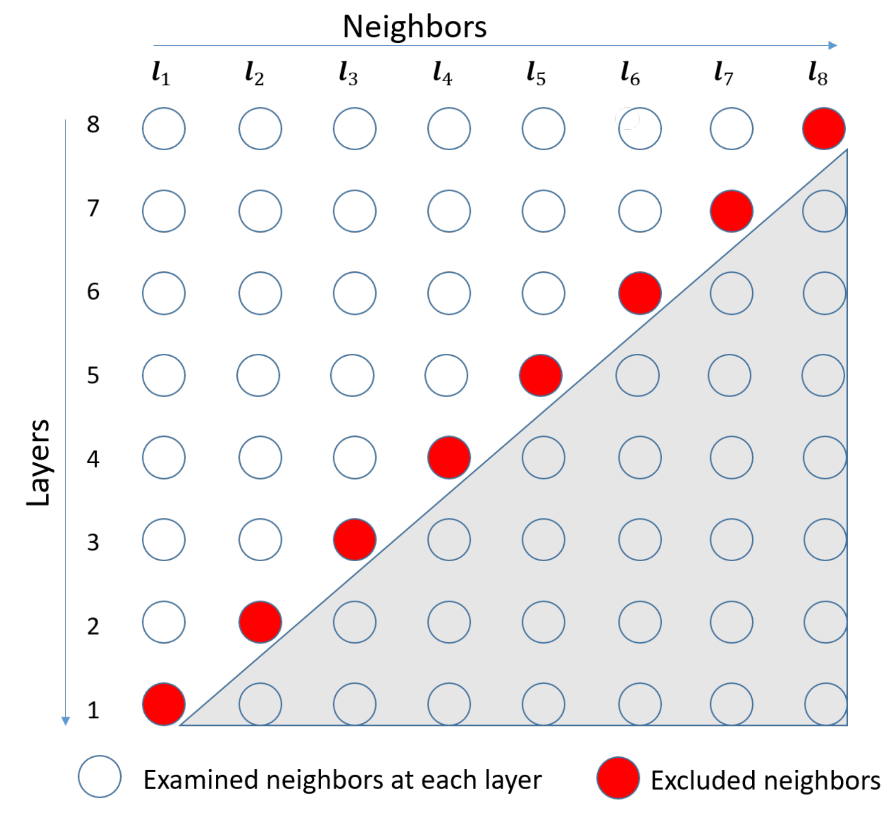
We develop a novel early neighbor rejection ENR-TS scheme. The TS algorithm computes the cumulative ML metrics of all the neighbors in each layer and rejects k neighbors whose cumulative metrics are larger than the others. The rejected neighbors are excluded from the computation of ML metrics in further layers, which reduces complexity.
2.
To mitigate the risk of excluding the best neighbor in early layers, we apply a layer ordering scheme, which sorts the layers of each neighbor in descending order of their expected metrics.
3.
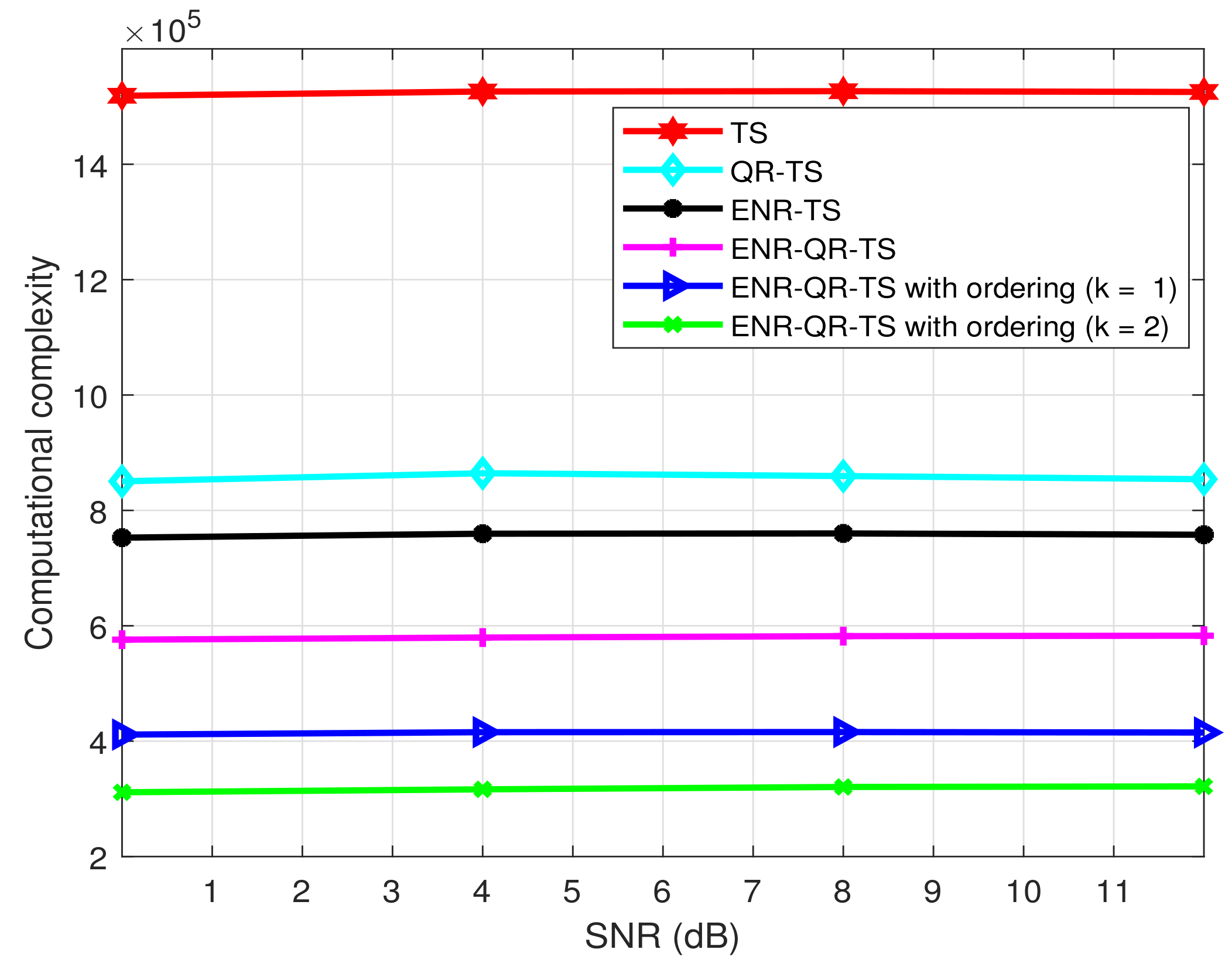
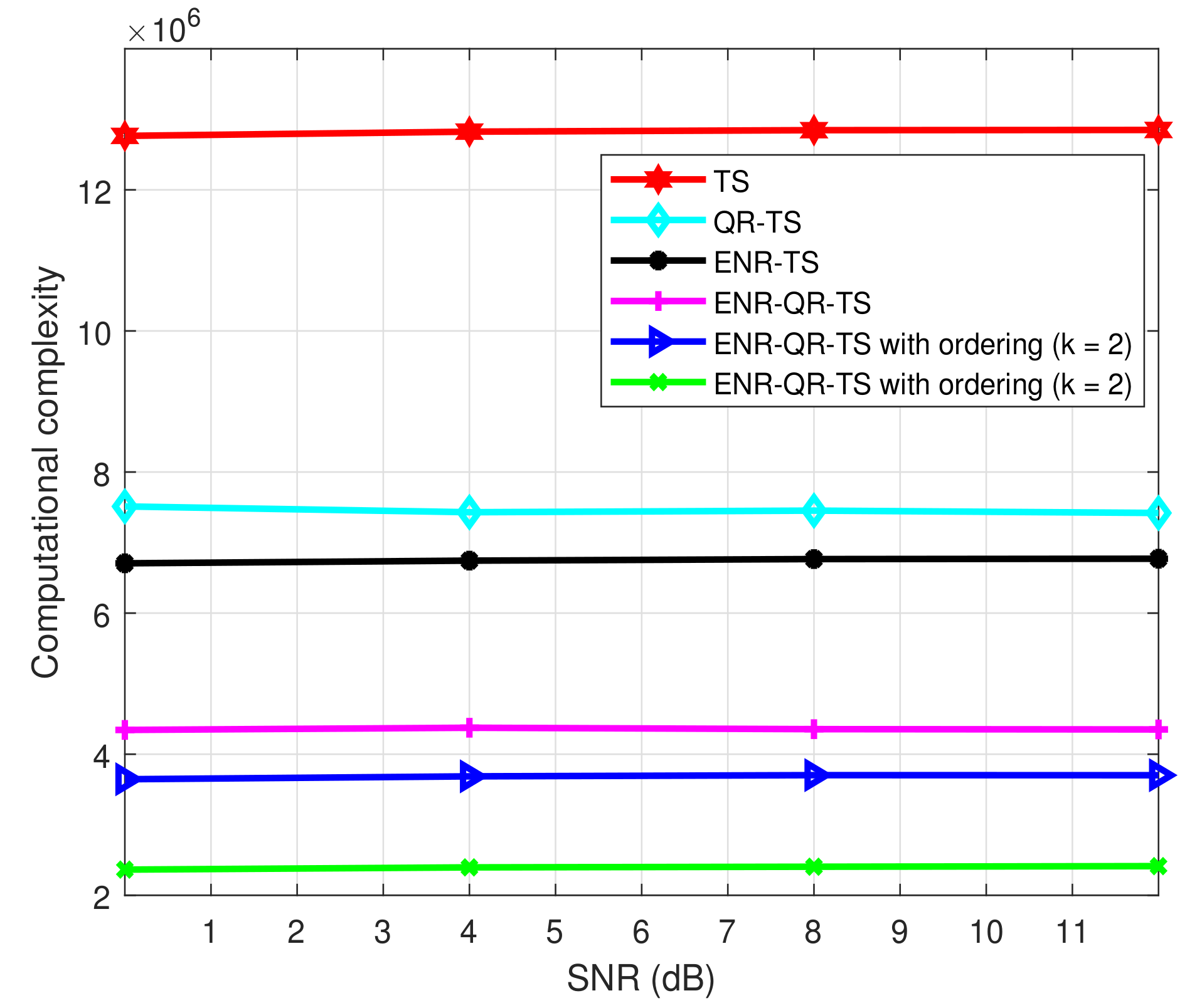
To evaluate the performance and complexity of the proposed scheme, we perform numerical analysis. The simulation results show that when the ERN scheme is incorporated into QR-TS (ENR-QR-TS), it reduces complexity by approximately 74% compared to the original TS scheme, while attaining almost the same BER performance.
The rest of this paper is organized as follows: in Section 2, the system model, conventional TS and QR-TS algorithms are described. In Section 3, the proposed ENR with QR-TS and ordering schemes are developed. In Section 4, the simulation results are presented. Finally, the conclusions of the study are presented in Section 5.
Notations: A boldface capital X is used to denote a matrix, and a boldface lowercase x represents a column vector. The entry in the ith row and jth column of X is denoted by x i , j , whereas the ith entry of vector x is denoted by x i . The jth column vector of X is denoted by x j . The transpose operation is denoted by ( · ) T , and the norm of a vector is denoted by · . Finally, ( · ) and ( · ) indicate the real and imaginary parts of a matrix or vector, respectively.

2. Background

2.1. MIMO System Description

In a MIMO system with N t transmit and N r receive antennas, the received signal vector y ˜ = [ y ˜ 1 , y ˜ 2 , , y ˜ N r ] T is given by
y ˜ = H ˜ s ˜ t + n ˜ ,
where s ˜ t = [ s ˜ t , 1 , s ˜ t , 2 , , s ˜ t , N t ] T is the transmitted signal vector with each component independently drawn from a complex constellation, such as quadrature amplitude modulation (QAM), and H ˜ denotes an N r × N t channel matrix, where h ˜ i , j is the complex channel gain between the jth transmit antenna and ith receive antenna. Furthermore, n ˜ = n ˜ 1 , n ˜ 2 , n ˜ N r T is a noise vector consisting of independent and identically distributed additive white Gaussian noise (AWGN) samples with zero mean and unit variance. We assume that the channel matrix is perfectly known at the receiver.
The complex system model (1) can be transformed to its equivalent real signal model y = H s t + n , i.e.,
( y ˜ ) ( y ˜ ) = ( H ˜ ) ( H ˜ ) ( H ˜ ) ( H ˜ ) ( s ˜ t ) ( s ˜ t ) + ( n ˜ ) ( n ˜ ) .
In (2), the dimension of the matrices and vectors doubles compared to (1), i.e., s t contains N = 2 N t elements, and the ( M × 1 ) -received signal vector y , ( M × N ) -channel matrix H , and ( M × 1 ) -noise signal vector n also double their dimensions, such that M = 2 N r .
Based on the signal model (2), the optimal solution s ^ ML can be determined as
s ^ ML = arg min s Ω N y Hs 2 ,
where y Hs 2 is the ML metric value for s , and Ω denotes the set of real entries in the constellation, e.g., Ω = { 3 , 1 , 1 , 3 } in the case of 16-QAM.

2.2. System Model

This paper considers a MIMO system with N t transmit and N r receive antennas. Let H ˜ C N r × N t denote the channel matrix, where h ˜ i , j is the complex channel gain between the jth transmit antenna and the ith receive antenna. Let s ˜ C N t × 1 be a transmit signal vector whose elements take values from a complex constellation A ˜ of QAM modulation. An N r × 1 received signal vector y ˜ is given by the complex signal model
y ˜ = H ˜ s ˜ + n ˜ ,
where n ˜ C N r × 1 is a noise vector consisting of independent and identically distributed (i.i.d.) complex additive white Gaussian noise (AWGN) samples with zero mean and unit variance σ n 2 .
The complex signal model (4) can be converted to its equivalent real signal model y = Hs + n , i.e.,
( y ˜ ) ( y ˜ ) = ( H ˜ ) ( H ˜ ) ( H ˜ ) ( H ˜ ) ( s ˜ ) ( s ˜ ) + ( n ˜ ) ( n ˜ ) ,
where there are N = 2 N t = 2 N r layers, y , x , and n are the ( N × 1 ) -equivalent real received, transmitted, and AWGN noise signal vectors, respectively, and H represents the ( N × N ) -equivalent real channel matrix. Finally, A = { ± 1 , ± 3 , Ω 1 } is the equivalent real-valued constellation set of A ˜ , where Ω indicates the modulation order of Ω -QAM signaling.
Based on the signal model in (5), the maximum likelihood (ML) solution can be expressed as
s ML = arg min s A N ϕ ( s ) ,
where A N is the set of all possible transmitted signal vectors and ϕ ( s ) = y Hs 2 is the ML metric of s . The computational complexity of the ML detection in (6) grows exponentially with N, which makes it computationally prohibitive for large MIMO systems in which N is large.

2.3. Conventional TS Algorithm

We will now briefly explain the basic concepts of a conventional TS algorithm [13,14], which are necessary for an understanding of the proposed algorithm. The TS algorithm starts the search process from a current solution x ( c ) , which is often set to the zero-forcing solution x ZF = H y , where H denotes the left Moore–Penrose pseudo-inverse of H . Neighboring signal vectors around x ( c ) are determined based on neighboring criteria [14,15]. In an iteration of the search process in TS, the neighborhood of x ( c ) is defined as a subset of vectors in A N that differ from x ( c ) in only one element. Specifically, the set of neighboring vectors x of x ( c ) can be expressed as
N ( x ( c ) ) = { x A N L , | x x ( c ) | = d m i n } ,
where L denotes a tabu list, which is a set of previously visited neighbors, and A N L denotes the set of candidate neighboring vectors, excluding the vectors which are in L . Finally, d m i n is the minimum distance between two constellation points. In each iteration, TS examines the neighbors of the current solution N ( x ( c ) ) and moves to the best neighbor x ( b ) , which has the smallest ML metric among the vectors neighboring N ( x ( c ) ) (even if the best neighboring vector is worse in terms of ML cost y Hx 2 than the x ( c ) ) [9]. Specifically, the best neighbor is given by
x ( b ) = arg min x N ( x ( c ) ) ϕ ( x ) .
Hence, in each iteration, the best neighbor x ( b ) is inserted into L to avoid cycling in the search process. If L is full, the element that was first inserted into L is released to make room for the new best neighbor.
In each iteration, the ML metric of x ( b ) , i.e., ϕ ( x ( b ) ) , is compared with that of the best solution found so far, which is denoted by ϕ ( x TS ) . Initially, ϕ ( x TS ) is set to ϕ ( x ZF ) . If ϕ ( x ( b ) ) is smaller than ϕ ( x TS ) , we then update ϕ ( x TS ) to ϕ ( x ( b ) ) . The TS algorithm generally terminates after a preset maximum number of iterations M, but we can employ early termination to reduce the overall complexity. In particular, we keep track of how many iterations have proceeded without any improvement, denoted by p, in the x TS . When p reaches its maximum p m a x , the TS algorithm is terminated and the final solution is determined to be the best found solution x TS  [15,16].
It is worth noting that the ML metric of x can be computed in a more computationally efficient form as
ϕ ( x ) = y Hx 2 = u + H Δ x 2 = u + h d δ d 2 ,
where u = y H x ( c ) , Δ x = x ( c ) x = 0 , , 0 , δ d , 0 , , 0 T has only one nonzero element, which is δ d = x d ( c ) x d , and h d is the dth column of H . Here, d is the index of the unique nonzero element in Δ x .

2.4. QR-TS

The main complexity load of the conventional TS algorithm comes from computing the metrics of the neighbors to find x ( b ) in each iteration. The ML metric in (9) can be rewritten as
ϕ ( x ) = i = 1 N | u i + h i , d δ d | 2 .
In (10), it is prohibitive to compute N terms, i.e., | u i + h i , d δ d | 2 , i = 1 , , N , in each iteration when N is large.
By applying QR decomposition to the channel matrix H , where Q and R are unitary and upper triangular matrices, respectively, computational complexity can be reduced. Specifically, the ML metric of ϕ ( x ) can be expressed as
ϕ ( x ) = y Hx 2 = Q T y Rx 2 = Q T y R ( x ( c ) Δ x ) 2 .
By defining z = Q T y R x ( c ) , ML metric (8) can be rewritten, as in [12],
ϕ ( x ) = z + R Δ x 2 = z + r d δ d 2
= i = 1 d | z i + r i , d δ d | 2 ϕ A + i = d + 1 N | z i | 2 ϕ B ,
where r d is the dth column of R . By accounting for the fact that in each iteration of (11), x ( c ) is the same for all neighboring vectors, ϕ B , in (13) needs to be computed only once and can be reused for all neighbors, which reduces the computational complexity of the search process [11]. However, the number of neighbors increases with N. Thus, the number of iterations to achieve near-optimal performance in TS also increases. This implies that the QR-TS scheme may be still computationally expensive in large MIMO systems, which motivates us to find a technique for the early rejection of unpromising neighbors from examination. In the next section, we propose early neighbor rejection (ENR) for this purpose. A layer ordering scheme is also applied to further reduce the complexity of the TS algorithm.

3. Proposed Low Complexity TS Algorithms

3.1. ENR with QR-TS

In each iteration of the conventional TS algorithm, the best neighbor x ( b ) is determined after all neighbors are examined. One drawback of this approach is that the ML metric in (13) must be computed even for unpromising neighbors. To exclude unlikely neighbors as early as possible, we propose an ENR-QR-TS, which performs a layer-by-layer search and excludes unpromising neighbor vectors from examination.
In the ENR-QR-TS, the neighbor examination starts from the Nth layer and proceeds to the final layer. At the Nth layer, each neighbor’s cumulative metric ϕ N ( x ) , which considers only the Nth layer, is computed. We then sort L neighbors, where L denotes the number of neighbors, in ascending order of their cumulative metrics and exclude k neighbors associated with the k largest cumulative metrics. Hence, in the ( N 1 ) th layer, we consider only ( L k ) retained neighbors. Similarly to the Nth layer, the cumulative metrics of the retained ( L k ) neighbors are updated for the ( N 1 ) th layer to determine which k neighbors will be excluded from the remaining procedure. The process to update the cumulative metric and exclude k neighbors is iterative. Specifically, at layer i, the cumulative metric ϕ i ( x ) is calculated as
ϕ i ( x ) = ϕ i + 1 ( x ) + | z i + r i , d δ d | 2 , i d ϕ i + 1 ( x ) + | z i | 2 , i > d .
We sort the cumulative metrics ϕ i ( x ) in ascending order and exclude the k neighbors corresponding to the k largest cumulative metrics. Thus, a larger k leads to lower complexity but also poor BER performance because it increases the risk of excluding the best neighbor. This means that the value of k determines the trade-off between complexity and performance.
Figure 1 illustrates the operation of the proposed ENR scheme for k = 1 when there are eight neighbors ( l 1 , , l 8 ) and eight layers ( 1 , , 8 ) . To more easily illustrate the operation, it is assumed that the neighbors are excluded in the order of ( l 8 , , l 1 ) . Figure 1 shows that at layer 8, all the neighbors are examined, i.e., all their cumulative metrics are computed. Assuming that neighbor l 8 has the largest cumulative metric, it is excluded from the rest of the process. At layer 7, the remaining seven neighbors’ metrics are computed, and neighbor l 7 is chosen for exclusion. This process continues to layer 1 until only one neighbor is left to be determined the best neighbor. In Figure 1, it can be observed that the complexity of this process is approximately half the complexity of the conventional TS because, on average, the cumulative metrics are computed for only half the neighbors in an iteration. However, this means there is a risk of excluding the best neighbor. This can happen in early layers when the cumulative metric of the best neighbor is larger than those of other neighbors even though its complete metric ϕ ( x ( b ) ) is the smallest among all neighbors. To mitigate this risk, we propose applying a layer ordering scheme to the ENR-QR-TS.

3.2. ENR-QR-TS with Layer Ordering

In the proposed ENR-QR-TS scheme, we exclude k neighbors associated with the largest cumulative metrics in each layer. If in the first layer, the cumulative metric of the best neighbor is larger than those of the other neighbors, it is excluded early by the ENR scheme, which leads to the selection of the wrong best neighbor. To avoid this undesired consequence, we should minimize the mismatch between the complete metric and cumulative metrics in early layers.
The expected metric of the ith layer can be rewritten as in [12], as
E | z i + r i , d δ d | 2 σ n 2 + | r i , d | 2 δ 2 ,
where σ n 2 is a constant and δ 2 = | δ d | 2 . In (15), it can be seen that the expected metric at layer i depends only on | r i , d | 2 . Furthermore, as | r i , d | 2 is larger, the expected metric of the ith layer is larger, which contributes more significantly to the complete metric. Therefore, to minimize the mismatch between the complete metric and the cumulative metrics in early layers, layers with a larger | r i , d | 2 need to be considered earlier.
Therefore, we rearrange the computation order in (14) such that the computations corresponding to a larger | r i , d | 2 are performed earlier. Layers with larger expected metrics are considered earlier in the computation of (14) to mitigate the chance of an early exclusion of the best neighbor.
In Algorithm 1, steps 1–6 correspond to layer ordering. Specifically, r d ̲ in step 3 denotes the dth column of the R that is sorted by its expected metric in descending order. When layer ordering is not applied, r d ̲ is set to the original r d in step 8. Steps 10–11 are for initializing the current solution with x ZF . Steps 12–32 represent the search process, which is incorporated with the ENR-QR-TS. Steps 27–29 correspond to checking the tabu list L ; if the tabu list if full, the first element is released to make a space for the current solution. Finally, steps 30–31 checks for the stopping criteria, such as p.
Algorithm 1 ENR-QR-TS with layer ordering.
INPUT: H , y , M
1:
Output: x TS
2:
if layer ordering is used then
3:
    for  i = 1 to L do
4:
        for  d = 1 to N do
5:
           Find r d ̲ by sorting the elements in r d in descending order of | r i , d | 2 .
6:
        end for
7:
    end for
8:
else
9:
     r d ̲ = r d
10:
end if
11:
x ZF = H y
12:
Initialize x TS = x ZF and x ( c ) = x ZF .
13:
for m = 1 to M do
14:
    Find the neighbor set N ( x ( c ) ) and the set of different positions D .
15:
     L = N ( x ( c ) )
16:
    for  i = 1 to N do
17:
        for  l = 1 to L do
18:
           Compute the ϕ i ( x ) in (14) for each neighbor x N ( x ( c ) )
19:
        end for
20:
        Exclude the neighbors with the k largest ϕ i ( x ) from N ( x ( c ) )
21:
        Update the number of neighbors: L = L k .
22:
    end for
23:
    Determine the best neighbor x ( b ) with the minimum metric.
24:
    Update the current solution as x ( c ) = x ( b ) , ϕ ( x ( c ) ) = ϕ ( x ( b ) )
25:
    if  ϕ ( x ( c ) ) < ϕ ( x TS )  then
26:
        Update the best solution as x TS = x ( c ) , ϕ ( x TS ) = ϕ ( x ( c ) ) .
27:
    end if
28:
    if Tabu list L is full then
29:
        Release the first element in L .
30:
    end if
31:
    Update the tabu list L with x ( c ) , p = p + 1
32:
    Check for the stopping criteria [15].
33:
end for

3.3. Complexity Analysis

In this section, we analyse the overall computational complexity of the proposed ENR-QRT-TS algorithms and the conventional TS.
(1) Initialization: To obtain the Q and R matrix, we used the QR Householder method, which costs 2 3 N 3 additions and 2 3 N 3 multiplications [17]. The computation of the initial solution x Z F = H y = R 1 Q T y requires N 2 + 1 2 N 2 + 1 2 N multiplications and N 2 N + 1 2 N 2 1 2 N additions. Computing the ML metric of the initial solution ϕ ( x ( c ) ) = Q T y R x ( c ) 2 required 1 2 N 2 + 1 2 N additions and 1 2 N 2 + 3 2 N multiplications. Therefore, the total computation cost of the initial solution is 2 3 N 3 + 2 N 2 N additions and 2 3 N 3 + 2 N 2 + 2 N multiplications.
(2) Neighbor search: The computation of z in (9) is only computed once in each iteration because z is the same for all neighbors. Therefore, the computational complexity of computing z is negligible and ignored in the following analysis. To find the best neighbor in (10) requires i = 1 L ( 2 N 1 ) L additions and 2 N L multiplications an average for a conventional TS. In addition, the ENR algorithm requires an average of L ( N + 1 ) comparisons in each iteration. The fairness of our complexity assessment used the same contribution in the TS iteration for all variants of TS. It is worth noting that the computational load of the iterative searching process is significantly higher than that of the initial computation and dominates the overall complexity.
(3) Layer ordering: The layer ordering scheme is performed in steps 1–6. In layer ordering, computing | r i , d | 2 , i = 1 , 2 , , d requires 1 2 d log 2 d comparisons and d multiplications on average using the quick-sort algorithm in [18]. Therefore, the total complexity of the layer ordering is d = 1 N ( d + 1 2 d l o g 2 d ) = 1 2 ( N 2 + N + l o g 2 H ( N ) ) flops, where H ( · ) denotes the hyperfactorial function of H [19]. The complexity cost of ENR-QR-TS is increases by employing the layer ordering method; however, the complexity reduction achieved by layer ordering is significant, as shown in Figures 4 and 5. The overall complexity of the conventional TS and QR-TS comes by only adding the initialization phase and iterative searching phase. In contrast, to compute the total complexty cost of the proposed ENR-TS algorithms are considered all three phases.

4. Simulation Results

In our experiments, the BER performance and computational complexity of the proposed ENR-TS with a layer ordering scheme were evaluated for various MIMO configurations. Although Section 3.1 describes the proposed ENR-QR-TS scheme, it can also be applied to the original TS without QR decomposition. In the simulation results, ENR-QR-TS represents the former and ENR-TS the latter. The ENR-QR-TS scheme can be incorporated with a layer ordering scheme, as explained in Section 3.2. The complexities of the proposed ENR-TS algorithms are compared with that of the conventional TS algorithm. The total computational complexity was measured by summing the average number of real multiplications, additions, comparisons, and sorting operations. In the simulations, we used two MIMO configurations: ( N r , N t , Ω ) = ( 16 , 16 , 4 ) and ( 32 , 32 , 4 ) , where the number of iterations M are 400 and 800, respectively. The number of excluded neighbors in each layer is k = 1 and 2.
Figure 2 shows the BER comparison results for a MIMO system with N r = 16 , N t = 16 and 4-QAM. We can observe that the performance of the proposed ENR-TS algorithms is almost the same as that of the conventional TS. Figure 3 compares the BER performance for N r = 32 , N t = 32 , and 4-QAM. Similarly to Figure 2, this figure demonstrates that the ENR-TS and ENR-QR-TS schemes achieve a BER performance nearly identical to that of conventional TS scheme. It is worth noting that the ENR-QR-TS algorithm with the layer ordering scheme also performs nearly as well as the conventional QR-TS. Moreover, the ENR-QR-TS scheme with k = 2 achieves comparable BER performance with respect to the conventional TS.
Figure 4 shows the complexity comparison for a MIMO system with N r = 16 , N t = 16 , and 4-QAM. Figure 4 shows that the ENR-QR-TS with layer ordering requires the lowest complexity of the compared schemes. Specifically, compared with the conventional TS, the ENR-QR-TS with layer ordering at SNR = 12 dB reduces complexity by approximately 73 % , while achieving almost the same BER performance. The QR-ENR-TS scheme provides a 33 % reduction in complexity compared with the conventional QR-TS.
Figure 5 illustrates the comparison of the complexity of a MIMO system with N r = 32 , N t = 32 , and 4-QAM. Similarly to Figure 4, this figure shows that the proposed ENR-QR-TS scheme reduces complexity significantly compared to the conventional TS and QR-TS algorithms. With layer ordering at SNR = 12 dB, the ENR-QR-TS with k = 2 reduces the complexity of the conventional TS by about 82 % . At SNR = 12 dB, the ENR-QR-TS scheme with k = 2 achieves a complexity reduction of approximately 70 % compared to the QR-TS.

5. Conclusions

In this study, a novel ENR-TS algorithm was proposed to reduce the computational complexity of TS for large MIMO systems. The proposed ENR-QR-TS scheme rejects the most unreliable neighbors in terms of their ML metric sequentially in each layer, which reduces the burden of complexity in the best neighbor search of TS. To further reduce the complexity of the ENR-QR-TS algorithm, an ordering scheme was also proposed. Specifically, the expected metrics of layers are sorted in descending order, so more unpromising neighbors are likely to be rejected earlier. The simulation results show that the proposed ENR-QR-TS algorithms achieved nearly the same BER performance as the conventional TS while substantially reducing complexity. ENR-QR-TS with layer ordering when k = 2 achieves a complexity reduction approximately 82 % , with respect to conventional TS.

Author Contributions

Data curation, U.U.; Investigation, U.U.; Methodology, U.U., J.-S.P., G.-J.J., J.-D.L.; Supervision, U.U.; Writing—original draft, U.U.; Writing—review and editing, U.U., J.-S.P., G.-J.J. and J.-D.L. All authors have read and agreed to the published version of the manuscript.

Funding

This research received no external funding.

Acknowledgments

This work was supported by the Institute of Information and Communications Technology Planning and Evaluation (IITP) grant funded by the Korean government (MSIT) (No. 2020-0-00158, Development of high power RF Front-End for 5G base band array antenna).

Conflicts of Interest

The authors declare no conflict of interest.

References

  1. Rusek, F.; Persson, D.; Lau, B.K.; Larsson, E.G.; Marzetta, T.L.; Edfors, O.; Tufvesson, F. Scaling up MIMO: Opportunities and challenges with very large arrays. IEEE Signal Process. Mag. 2013, 30, 40–60. [Google Scholar] [CrossRef] [Green Version]
  2. Zanella, A.; Chiani, M.; Win, M.Z. MMSE reception and successive interference cancellation for MIMO systems with high spectral efficiency. IEEE Trans. Wirel. Commun. 2005, 4, 1244–1253. [Google Scholar] [CrossRef] [Green Version]
  3. Hassibi, B.; Vikalo, H. On the sphere-decoding algorithm I. Expected complexity. IEEE Trans. Signal Process. 2005, 53, 2806–2818. [Google Scholar] [CrossRef] [Green Version]
  4. Guo, Z.; Nilsson, P. Algorithm and implementation of the K-best sphere decoding for MIMO detection. IEEE J. Sel. Areas Commun. 2006, 24, 491–503. [Google Scholar]
  5. Ummatov, U.; Lee, K. Adaptive Threshold-Aided K-Best Sphere Decoding for Large MIMO Systems. Appl. Sci. 2019, 9, 4624. [Google Scholar] [CrossRef] [Green Version]
  6. Albreem, M.A.; Juntti, M.; Shahabuddin, S. Massive MIMO detection techniques: A survey. IEEE Commun. Surv. Tutor. 2019, 21, 3109–3132. [Google Scholar] [CrossRef] [Green Version]
  7. Tseng, S.M.; Lee, H.L. An adaptive partial parallel multistage detection for MIMO systems. IEEE Trans. Commun. 2005, 53, 587–591. [Google Scholar] [CrossRef]
  8. Yang, S.; Hanzo, L. Fifty years of MIMO detection: The road to large-scale MIMOs. IEEE Commun. Surv. Tutor. 2015, 17, 1941–1988. [Google Scholar] [CrossRef] [Green Version]
  9. Datta, T.; Srinidhi, N.; Chockalingam, A.; Rajan, B.S. Random-restart reactive tabu search algorithm for detection in large-MIMO systems. IEEE Commun. Lett. 2010, 14, 1107–1109. [Google Scholar] [CrossRef]
  10. Srinidhi, N.; Datta, T.; Chockalingam, A.; Rajan, B.S. Layered tabu search algorithm for large-MIMO detection and a lower bound on ML performance. IEEE Trans. Commun. 2011, 59, 2955–2963. [Google Scholar] [CrossRef]
  11. Nguyen, N.T.; Lee, K. Groupwise Neighbor Examination for Tabu Search Detection in Large MIMO Systems. IEEE Trans. Veh. Technol. 2019, 69, 1136–1140. [Google Scholar] [CrossRef] [Green Version]
  12. Nguyen, N.T.; Lee, K.; Dai, H. QR-Decomposition-Aided Tabu Search Detection for Large MIMO Systems. IEEE Trans. Veh. Technol. 2019, 68, 4857–4870. [Google Scholar] [CrossRef]
  13. Srinidhi, N.; Mohammed, S.K.; Chockalingam, A.; Rajan, B.S. Low-complexity near-ML decoding of large non-orthogonal STBCs using reactive tabu search. IEEE Int. Symp. Inf. Theory 2019, 17, 1993–1997. [Google Scholar]
  14. Srinidhi, N.; Mohammed, S.K.; Chockalingam, A.; Rajan, B.S. Near-ML signal detection in large-dimension linear vector channels using reactive tabu search. arXiv 2009, arXiv:0911.4640. [Google Scholar]
  15. Zhao, H.; Long, H.; Wang, W. Tabu search detection for MIMO systems. In Proceedings of the IEEE 18th International Symposium on Personal, Indoor and Mobile Radio Communications, Athens, Greece, 3–7 September 2007; pp. 1–5. [Google Scholar]
  16. Glover, F. Tabu search—Part I. ORSA J. Comput. 1989, 1, 190–206. [Google Scholar] [CrossRef] [Green Version]
  17. Golub, G.H.; Van Loa, C.F. Matrix Computations; JHU Press: Baltimore, MD, USA, 2012; Volume 3. [Google Scholar]
  18. Sedgewick, R. Implementing quicksort programs. Commun. ACM 1978, 21, 847–857. [Google Scholar] [CrossRef]
  19. Agrell, E.; Eriksson, T.; Vardy, A.; Zeger, K. Closest point search in lattices. IEEE Trans. Inf. Theory 2002, 48, 2201–2214. [Google Scholar] [CrossRef] [Green Version]
Figure 1. The ENR operation for k = 1 and L = 8.
Applsci 11 07305 g001
Figure 2. Comparison of the BER performance of TS algorithms for a 16 × 16 MIMO system with 4-QAM.
Applsci 11 07305 g002
Figure 3. Comparison of the BER performance of TS algorithms for a 32 × 32 MIMO system with 4-QAM.
Applsci 11 07305 g003
Figure 4. Comparison of the computational complexity of TS algorithms for a 16 × 16 MIMO system with 4-QAM.
Applsci 11 07305 g004
Figure 5. Comparison of the computational complexity of TS algorithms for a 32 × 32 MIMO system with 4-QAM.
Applsci 11 07305 g005
Publisher’s Note: MDPI stays neutral with regard to jurisdictional claims in published maps and institutional affiliations.

