Repositioning Bikes with Carrier Vehicles and Bike Trailers in Bike Sharing Systems

Abstract

Bike sharing systems (BSSs) are widely adopted in major cities of the world due to traffic congestion and carbon emissions. Although there have been approaches to exploit either bike trailers via crowdsourcing or carrier vehicles to reposition bikes in the “right” stations in the “right” time, they did not jointly consider the usage of both bike trailers and carrier vehicles. In this paper, we aim to take advantage of both bike trailers and carrier vehicles to reduce the loss of demand by determining whether bike trailers or carrier vehicles (or both) should be used. In addition, we also would like to maximize the overall profit with regard to the crowdsourcing of bike trailers and the fuel cost of carrier vehicles. In the experiment, we exhibit that our approach outperforms baselines in multiple data sets from bike sharing companies.

1. Introduction

Bike sharing systems (BSSs) typically have a set of base stations that are strategically placed throughout a city and each station has a fixed number of docks. At the beginning of the day, each station is stocked with a predetermined number of bikes. Customers can pick and drop bikes from any station and are charged depending on the hiring duration. BSSs are capable of providing healthier living and greener environments while delivering fast movements for customers [1,2,3,4,5], e.g., Capital Bikeshare in Washington DC, Hubway in Boston, Mobike in Hangzhou, BIXI in Montréal, etc.

Due to the individualistic and uncoordinated movements of customers, there is often starvation (empty base stations precluding bike pickup) or congestion (full base stations precluding bike return) of bikes at certain stations, which results in a significant loss of customer demand [6,7]. To address this problem, a variety of systems [3,8] employ the idea of repositioning idle bikes with the help of carrier vehicles [1,9] during the day, by taking into account the movement of bikes by customers [10]. While above solutions of repositioning can help reduce imbalance, repositioning idle bikes using carrier vehicles incurs substantial routing and fuel costs while covering entire stations (The carrier vehicle is a truck to reposition idle bikes during the day using myopic and ad hoc methods so as to return to a predetermined configuration (e.g., each carrier vehicle can hold 30–40 bikes, its working distance is 5 km away)), as done by [11]. In addition, repositioning idle bikes using bike trailers just carries a few of bikes once and the range is limited (The bike trailer is an add-on to a bike that can carry a small number of bikes (e.g., each bike trailer can hold 4–6 bikes, its working distance is within 5 km) and is useful to relocate bikes to nearby stations). Meanwhile, they failed to take into account the available budget [8], working distance (Since nearby stations can be covered by bike trailers, we exploit the geographical-proximity-based clustering method to obtain main stations to reduce the usage of carrier vehicles) and carrying capacity [12,13], which may restrict the usage of bike trailers.

In this paper, we propose an optimization model called (DRRPVT), which stands for Dynamically Repositioning and Routing Problem with carrier Vehicles and bike Trailers, to jointly consider the usage of carrier vehicles and bike trailers. We aim to better match the overall profit of hired bikes and consequently reduce the expected lost demand. Specifically, we build a profit objective function to calculate the value of carrier vehicle routing (i.e., fuel cost) and bike trailers (i.e., payment for the users of bike trailers), by considering a variety of constraints with respect to carrier vehicle routing and bike repositioning. Jointly considering both carrier vehicles and bike trailers is challenging in the sense so that we need to introduce new constraints to consider both carrier vehicles and bike trailers, and build a novel objective function to minimize the value of repositioning (and routing) and the loss of demand. To improve the efficiency of our approach with respect to large-scale problem with many stations (carrier vehicles and bike trailers), we design a clustering mechanism for computing main base stations to help reduce the computation time.

In summary, our novel contributions can be described by three aspects:

• We propose an optimization model to improve upon the prior literature by bringing in simultaneous use of both carrier vehicles and bike trailers in the context of dynamic repositioning. While dynamic repositioning has been considered for bike trailers and carrier vehicles separately, previous work has not been considered jointly.
• We propose a new profit objective function and additional constraints considering both carrier vehicles and bike trailers to reduce lost customer demand and increase overall profits. While profit objective function has been considered for reduce lost customer demand and increase overall profits separately, previous work has not been considered jointly.
• We design a clustering mechanism for computing main base stations to help improve the efficiency of optimization model with respect to large-scale problem with many stations.

2. Related Work

There have been many approaches proposed to deal with bike sharing problems, which can be categorized into three aspects [1,14,15,16], i.e., static repositioning using carrier vehicles, dynamic repositioning using carrier vehicles, and dynamic repositioning using bike trailers.

2.1. Static Repositioning Using Carrier Vehicles

Static repositioning is the problem of finding routes for a fleet of vehicles to reposition bikes at the end of the day when the movements of bikes by customers are negligible, to achieve a predetermined inventory level at the stations [17]. Gaspero et al. provided constraint programming to efficiently solve static repositioning using large neighborhood search [18]. As user demands change frequently during the day, those approaches are not capable of dynamically adjusting the station inventory level with respect to user demands. Furthermore, Szeto et al. provided a novel set of loading and unloading strategies and further embeds them into an enhanced artificial bee colony algorithm to solve the bike repositioning problem.

2.2. Dynamic Repositioning Using Carrier Vehicles

To consider dynamic repositioning using carrier vehicles with respect to the movements of customers during the day, Lowalekar et al. provided a scalable online repositioning solution using multistage stochastic optimization with online anticipatory algorithms [3,19]. Pierre et al. developed a efficient mechanism to maximize the decision intervals between repositioning events by online rebalancing operations [2,7]. Ghosh et al. proposed a dynamic bike repositioning approach based on a probabilistic satisficing method that uses the uncertain demand parameters that are learned from historical data [14]. Furthermore, many approaches rely on clustering to simplify the problem complexity. Ruffieux et al. provided a prediction module forecasts bikes availability at the station level using machine learning and the rebalancing module provides optimal rebalancing operations and routes using constraint programming [12]. Meanwhile, many approaches rely on predicting the quantity of bikes in advance to perform the dynamic rebalancing. Liu et al. proposed an adaptive capacity constrained k-centers clustering algorithm to separate outlier stations and group the remaining stations into clusters within which one vehicle is scheduled to redistribute bikes between stations [13]. As dynamic repositioning using vehicles alone incurs substantial routing and fuel cost, those approaches should be improved to be self-sustaining and environmentally friendly.

2.3. Dynamic Repositioning Using Bike Trailers

To consider the self-sustaining and environment issues, instead of using vehicles, Ghosh et al. proposed a pricing mechanism that takes the global view of the repositioning requirements and incentives the execution of bike trailer tasks (based on crowdsourcing) within the budget constraints [10,20]. Liu et al. proposed a centralized pricing-based dynamic incentive mechanism to mobilize the participants via crowdsourcing with regarding to reposition the indiscriminately parked bikes [21]. Despite the success of those approaches, bike trailers can only take a few bikes at once and the distance of movements is limited. To bridge this gap, Liu et al. proposed an ethically aligned incentive optimization approach that maximizes the rate of success for bike repositioning while minimizing cost and prioritizing users’ wellbeing [15]. Furthermore, Liu et al. developed a meteorology similarity weighted k-nearest neighbor regressor to predict the station pickup demand based on large-scale historic trip records and proposed an interstation bike transition model to predict the station drop-off demand [18]. The value of crowdsourcing tasks may be high (over the available budget).

Different from previous approaches, our DRRPVT approach aims to leverage the advantage of using both carrier vehicles, which are able to take a large number of bikes and move to longer distance, and bike trailers, which are able to move to short distance with limited cost and allow self-sustaining, by considering the expected profit and the loss demands reduction of repositioning and routing solution [22,23].

3. Problem Formulation

Our bike sharing problem is formally defined by the following tuple:

$$\langle \mathcal{S},\mathcal{V},\mathcal{F},{\mathcal{C}}^{\#},{\mathcal{C}}^{*},d^{\#},d^{*},\sigma ,R,P,\widehat{P},D,B\rangle ,$$

where

• $\mathcal{S}$ denotes the set of base stations.
• $\mathcal{V}$ denotes the set of vehicles used for repositioning, which is restricted to carrier vehicles only.
• $\mathcal{F}$ denotes samples of customer requests for the future time steps with $F_{s,s^{\prime }}^t$ indicating the number of customer requests between stations s and $s^{\prime }$, which start at decision epoch t and end at decision epoch $t+1$.
• ${\mathcal{C}}^{\#}$ denotes the capacity of stations with $C_s^{\#}$ indicating capacity of station s.
• ${\mathcal{C}}^{*}$ denotes the capacity of carrier vehicles or bike trailers with $C_v^{*}$ indicating capacity of vehicle v or bike trailer v.
• $d^{\#}$ denotes the distribution of bikes at stations with $d_s^{\#,t}$ indicating the number of bikes at station s at decision epoch t.
• $d^{*}$ denotes the distribution of bikes in vehicles with $d_v^{*,t}$ indicating the number of bikes in vehicle v at decision epoch t.
• $\sigma$ denotes the distribution of carrier vehicles at stations, with ${\sigma }_{v,s}^t$ set to be 1 if vehicle v is present at station s at decision epoch t and 0 otherwise.
• R denotes the revenue of bikes being hired, with $R_{s,s^{\prime }}^t$ indicating the revenue from station s to $s^{\prime }$ which starts at decision epoch t and ends at decision epoch $t+1$.
• D denotes the actual distance with $D_{s,s^{\prime }}$ indicating the distance between stations s and $s^{\prime }$.
• B denotes the total budget for all trailers to bid. In other words, the total amount of value spent on trailers should not be larger than B.
• $\widehat{P}$ denotes the value for executing the task of bike trailer with ${\widehat{P}}_{s,s^{\prime }}$ indicating the value for executing the task of bike trailer picking up idle bikes at station s and dropping off them at station $s^{\prime }$.
• P denotes the routing value (e.g., fuel cost) for vehicles traveling with $P_{s,s^{\prime }}$ indicating the routing value for vehicles traveling from station s to $s^{\prime }$, which depends on the distance between the two stations.

We made the following assumptions for the ease of explanation and representation:

• We assumed that users who carry bikes and trailers at decision epoch t always return their bikes at the beginning of the decision epoch $t+1$. The duration of each decision epoch was 30 min. We evaluated different duration impacts on runtime performance. We chose 30 min as the default setting for the duration of time step.
• We sampled the empirical distribution of the real historical data of customer requests to simulate customer requests for the future time steps. We produced three types of demand scenarios: (1) We took the real demand data for 60 weekdays. We used 20 days of demand scenarios for training purpose and other 40 days of demand for testing. (2) We generated 100 demand scenarios, where the arrival demand at each station is generated using Poisson distribution with the mean computed from historical data. Similar to Shu et al. [6], we assume that customers reach their destination station with a fixed probability. (3) We generated 100 demand scenarios, where demand for each origin destination [OD] pair at each time step is computed using Poisson distribution. For the demand scenario types 2 and 3, we used 30 demand scenarios for training and 70 demand scenarios for testing [9]. We assumed that the numbers of extra bikes is the lost demand at the time of return. To ensure that the capacity constraints were considered for the stations, we transferred extra bikes to the nearest available station if the number of bikes exceeds the station capacity. Once the distribution of bikes across the stations for time step $t+1$ was obtained, we utilized this information to compute the repositioning strategy for trailers and vehicles for time step $t+1$. This iterative process continued until we reached the last decision epoch.
• Customers can rent a bike for 30 min or more, and they have to know in advance at which station they will return the bike. On the other hand, they return their bikes to the nearest available station if the destination station is full, and they leave the system if they encounter an empty station.

The goal of our DRRPVT approach is to maximize the expected profit over the entire time horizon. Let U denote the sum of revenue of hired bikes and the fuel cost of vehicles and the value of bike trailers. We provide an optimization model for a given DRRPVT. Specifically, we provide a mixed integer linear programming (MILP for short) that computes a profit-maximizing repositioning and routing solution. The objective is shown in Equation (1):

$$\begin{array}{c}{max}_{y,z,a,b}U={max}_{y,z,a,b}{\sum }_{s,s^{\prime },t}{R}_{s,s^{\prime }}^t\times x_{s,s^{\prime }}^t-{\sum }_{t,v,s,s^{\prime }}{b}_{s,s^{\prime },v}^t\times {\widehat{P}}_{s,s^{\prime }-{\sum }_{t,v,s,s^{\prime }}{P}_{s,s^{\prime }}\times z_{s,s^{\prime },v}^t}\\ s.t.constraintsC1\text{–}C15whichdependsony,z,a,b.\end{array}$$

(1)

Objective: To represent the trade-off between lost demand (or alternatively the revenue from customer trips) and the value $\widehat{P}$ of bike trailers and the value P of using carrier vehicles, we employ the dollar value of both quantities and combine them into the overall profit at any decision epoch in Expression (1). The notation used in the formulation are shown:

• $y_{s,v}^{+,t}$ denotes the number of bikes picked up from station s by vehicle v at decision epoch t.
• $y_{s,v}^{-,t}$ denotes the number of bikes dropped at station s by vehicle v at decision epoch t.
• $z_{s,s^{\prime },v}^t$ denotes whether vehicle v picks up bikes from station s at decision epoch t and drops off at station $s^{\prime }$ at decision epoch $t+1$.
• $a_{s,v}^{+,t}$ denotes the number of bikes picked up from station s by bike trailer v at decision epoch t.
• $a_{s,v}^{-,t}$ denotes the number of bikes dropped off at station s by bike trailer v at decision epoch t.
• $b_{s,s^{\prime }v}^t$ denotes a binary decision variable that is set to be 1 if bike trailer v picks up bikes from station s in at decision epoch t and returns bikes to station $s^{\prime }$ in at decision epoch $t+1$ else 0 otherwise.
• $x_{s,s^{\prime }}^t$ denotes the number of hired bikes moving from station s at decision epoch t to station $s^{\prime }$ at decision epoch $t+1$.

4. Constraints

In this section, we address the constraints (C1–C15) that we exploit in our bike sharing system, where constraints (C1–C4) are newly created in this paper, while constraints (C5–C8) have presented by [3,8] and constraints (C9–C15) have presented by [10].

4.1. C1: Preservation of Bike Flows in and Out of Station

We require that the bike flows in and out of stations should ensure that the number of bikes $d_s^{\#,t+1}$ is equivalent to the sum of bikes $d_s^{\#,t}$ in the previous time step and the net number of bikes coming into the station during that time step, i.e., for each station s and epoch t,

$$d_s^{\#,t+1}=d_s^{\#,t}+\sum _{\tilde{s}}{x}_{\tilde{s},s}^{t-1}-\sum _{s^{\prime }}{x}_{s,s^{\prime }}^t+\sum _v(y_{s,v}^{-,t}-y_{s,v}^{+,t}+a_{s,v}^{-,t}-a_{s,v}^{+,t})$$

where the net number is defined by the last three components.

4.2. C2: Preservation of Bikes Flows between Any Two Stations Follow the Transition Dynamics Observed in the Data

As a subset of arrival demand can be served if the number of bikes present in a station is less than the arrival demand, we require that bikes flows between station s and $s^{\prime }$ should be less than the product of the number of bikes present in the source station s ($d_s^{\#,t}$) and the transition probability that a bike will move from s to $s^{\prime }$ according to expected customer demand, i.e., for each $t,s,s^{\prime }$,

$$x_{s,s^{\prime }}^t\le d_s^{\#,t}\times \frac{F_{s,s^{\prime }}^t}{{\sum }_{\tilde{s}}{F}_{s,\tilde{s}}^t}.$$

4.3. C3: Value of Task for Bike Trailer

We require a mechanism for crowdsourcing the repositioning tasks to the users of bike trailers and generating a payment method to ensure that the users bid for the tasks truthfully. The valuation of trailer v task is proportional to the expected lost demand reduced by the trailer job in the training demand scenario ($\xi$ represents unit value of lost demand to compute overall value), i.e., for each $s,s^{\prime },t$,

$${\widehat{P}}_{s,s^{\prime }}^t=\xi \times \sum _{s,s^{\prime }}(F_{s,s^{\prime }}^t-d_s^{\#,t}).$$

4.4. C4: Ensuring the Budget Feasibility

We require to incentive compatibility over all tasks without violating the fix budget B feasibility. Each task of trailers $v\in V$ has a valuation for the task is denoted by $\widehat{P}$. We aim to allocate the tasks in a fashion that maximizes the overall valuation of the center while the total payment is bounded by the given budget B, i.e.,

$$\sum _{s,s^{\prime },v}{b}_{s,s^{\prime },v}^t\times {\widehat{P}}_{s,s^{\prime }}^t\le B.$$

4.5. C5: Preservation of Bikes Flows in and Out of Vehicles

We require that the number of bikes in a vehicle at a time step ($d_v^{*,t+1}$) is equivalent to the sum of the number of bikes in the vehicle at the previous time step ($d_v^{*,t}$) and the net number of bikes coming into the vehicle during that time step (${\sum }_s(y_{s,v}^{+,t}-y_{s,v}^{-,t})$, i.e., for each $v,t$,

$$d_v^{*,t}+\sum _s(y_{s,v}^{+,t}-y_{s,v}^{-,t})=d_v^{*,t+1}.$$

4.6. C6: Preservation of Vehicles Flows in and Out of Stations

We require that the number of vehicles going out of station s (${\sum }_s^{\prime }{z}_{s^{\prime },s,v}^{t-1}$) plus the number of vehicles present at station s at time epoch $t-1$ (${\sigma }_{s,v}^{t-1}$) is equivalent to the sum of the number of vehicles coming into station s (${\sum }_s^{\prime }{z}_{s,s^{\prime },v}^t$) and the vehicles which are present at station s at time epoch t (${\sigma }_{s,v}^t$). Note that one of ${\sum }_s^{\prime }{z}_{s,s^{\prime },v}^t$ and ${\sigma }_{s,v}^t$ could be one at most, i.e., for each $t,s,v$,

$$\sum _s^{\prime }{z}_{s,s^{\prime },v}^t+{\sigma }_{s,v}^t=\sum _s^{\prime }{z}_{s^{\prime },s,v}^{t-1}+{\sigma }_{s,v}^{t-1}.$$

4.7. C7: A Maximum of One Vehicle Can Be Present in One Station at Any Time Step

Due to limited space availability near base stations and to avoid a synchronization issue in pickup or drop-off events by multiple vehicles from the same station at the same time step, we require that the maximum number of vehicles at a station (${\sum }_{s^{\prime },v}{z}_{s,s^{\prime }v}^t$) less than 1, i.e., for each $t,s$,

$$\sum _{s^{\prime },v}{z}_{s,s^{\prime },v}^t\le 1.$$

4.8. C8: Vehicles Can Only Pick Bikes Up or Drop Bikes Off at a Station If They Are Present at That Station

We require that the number of bikes picked up or dropped off at station at each time step by each vehicle is bounded by whether the station is visited by the vehicle at that time step or not, i.e., for each $s,v,t$,

$$y_{s,v}^{+,t}+y_{s,v}^{-,t}\le C_v^{*}\times \sum _{s^{\prime }}{z}_{s,s^{\prime },v}^t.$$

4.9. C9: Trailer Capacity Is Not Exceeded While Picking Up Bikes

We require that the number of bikes picked up by trailer v from station s is bounded by the minimum value between the number of bikes present in the station and the capacity of the trailer, i.e., for each $s,v,t$,

$$a_{s,v}^{+,t}\le \sum _{s^{\prime }}{b}_{s,s^{\prime },v}^t\times min(d_s^{\#,t},C_v^{*}).$$

4.10. C10: Total Number of Bikes Picked Up from a Station Is Less Than the Number of Available Bikes

As multiple trailers can pick up bikes from the same station, we require that the total number of picked up bikes by all the trailers from station s during the planning period t is bounded by the number of bikes present at the station ($d_s^{\#,t}$), i.e., for each $s,t$,

$$\sum _v{a}_{s,v}^{+,t}\le d_s^{\#,t}.$$

4.11. C11: Station Capacity Is Not Exceeded While Dropping Off Bikes

We require that the total number of dropped off bikes at station s is bounded by the number of available slots for bikes at that station, i.e., for each $s,t$,

$$\sum _v{a}_{s,v}^{-,t}\le C_s^{\#}-d_s^{\#,t}.$$

4.12. C12: Total Traveling Distance for a Trailer Is Bounded by a Threshold Value

To represent the physical limitation of route, we need to ensure that the total distance traveled by a trailer in a given planning period is within a few kilometers. We require that the distance between pickup station and the drop-off station for a trailer v is bounded by a threshold value, $D_{max}$, i.e., for each $s,s^{\prime },v,t$,

$$b_{s,s^{\prime },v}^t\times D_{s,s^{\prime }}\le D_{max}.$$

4.13. C13: A Trailer Can Only Pick Bikes Up or Drop Bikes Off at Exactly One Station

We require that a trailer can go to exactly one station starting from a specific station, i.e., for each $v,t$,

$$\sum _{s,s^{\prime }}{b}_{s,s^{\prime },v}^t=1.$$

4.14. C14: A Trailer Should Return the Exact Number of Bikes Picked Up

We require that the number of bikes dropped off by a bike trailer in a station is exactly equals to the number of picked up bikes if the station is visited, i.e., for each $s^{\prime },v,t$,

$$a_{s^{\prime },v}^{-,t}=\sum _s(b_{s,s^{\prime },v}^t\times a_{s,v}^{+,t}).$$

Note that the above equations are nonlinear in nature. However, one component in the right hand side is a binary variable. Therefore, we can easily linearize them using the following formula, i.e., for each $s^{\prime },v,t$,

$$a_{s^{\prime },v}^{-,t}\le C_v^{*}\times \sum _s{b}_{s,s^{\prime },v}^t,$$

$$a_{s^{\prime },v}^{-,t}\le \sum _s{a}_{s,v}^{+,t},$$

$$a_{s^{\prime },v}^{-,t}\ge \sum _s{a}_{s,v}^{+,t}-(1-\sum _s{b}_{s,s^{\prime },v}^t)\times C_v^{*}.$$

4.15. C15: Station and Vehicle Capacities Are Not Exceeded When Repositioning Bikes

We require that the number of bikes at a station s does not exceed the number of available docks at that station ($C_s^{\#}$). Similarly, these constraints also enforce that the number of bikes picked up or dropped off by a vehicle v in aggregate does not exceed the capacity of the vehicle ($C_v^{*}$), i.e.,

$$0\le x_{s,v}^t\le F_{s,v}^t;0\le d_s^{\#,t}\le C_s^{\#};0\le d_v^{*,t}\le C_v^{*},$$

$$0\le y_{s,v}^{+,t},a_{s,v}^{+,t}\le d_s^{\#,t};0\le y_{s,v}^{-,t},a_{s,v}^{-,t}\le C_s^{\#}-d_s^{\#,t},$$

$$0\le y_{s,v}^{+,t},y_{s,v}^{-,t},a_{s,v}^{+,t},a_{s,v}^{-,t}\le C_v^{*};z_{s,v}^t,b_{s,s^{\prime },v}^t\in \left\{0,1\right\}.$$

Given constraints C1–C15, our task is to calculate which vehicles reposition bikes from state s to $s^{\prime }$, i.e., z, and which trailers reposition bikes from s to $s^{\prime }$, i.e., b, by optimizing Equation (1).

5. Our DRRPVT Approach

In order to solve Equation (1), we use the well-known Lagrangian dual decomposition (LDD) (Fisher, 1985; Gordon, et al., 2012) technique. While this is a general purpose approach, its scalability, usability, and utility depend significantly on the following characteristics of the model:

• Identifying the right constraints to be dualized: This step is crucial to ensure that the resulting subproblems are easy to solve and the resulting bound derived from the dual solution is tight during the LDD process. If the right constraints are not dualized, then the underlying Lagrangian-based optimization may not be decomposable or it may take significantly more time than the original MILP to find the desired solution.
• Extraction of a primal solution from an infeasible dual solution: The primal extraction process is important to derive a valid bound (heuristic solution) during the LDD process. In many cases, the solution obtained by solving the decomposed dual slaves can be infeasible with respect to the original formulation and, hence, the overall approach can potentially lead to slower convergence and poor solutions.
• Decompose the original problem into a master problem and two slaves: As highlighted in Equation (1), only constraints (8) contain a dependency between routing and repositioning variables. We dualize constraints (8) using the dual variables, ${\alpha }_{s,t,v}$ and obtain the Lagrangian function as Equation (2).

We exploit Lagrangian dual decomposition (called LDD) to provide a near optimal solution for the dynamic repositioning of bikes [3,8]. Although the LDD framework was indeed used in Ghosh et al., 2015 and 2017, challenging to investigate the usage of LDD to accommodate the new constraints. An overview of DRRPVT is shown in Algorithm 1. We will present the main steps of Algorithm 1 in the following subsections.

Algorithm 1 An overview of our DRRPVT approach

Input:$\langle \mathcal{S},\mathcal{V},\mathcal{F},{\mathcal{C}}^{\#},{\mathcal{C}}^{*},d^{\#},d^{*},\sigma ,P,\widehat{P},R,D,B\rangle$ Output: $y,z,a,b$   1: $\tilde{S}=CalculateMainStations$($\mathcal{S},D$)   2: $\alpha =0$, $iter=0$   3: while$[p-(\rho 1+\rho 2)]\le \delta$do   4:  $\rho 1,y,a,b\leftarrow SolveReposition({\alpha }^{iter})$   5:  $\rho 2,z\leftarrow SolveRouting({\alpha }^{iter})$   6:  ${\alpha }^{iter+1}\leftarrow {[{\alpha }^{iter}+\gamma \times (y^{+}+y^{-}-C^{*}\times {\sum }_{\tilde{S}}{z}_{·,\tilde{s},·})]}_{+}$   7:  $p,y_p,a_p,b_p\leftarrow ExtractPrimal(z)$   8:  $iter\leftarrow iter+1$   9: end while   10: $SolvingIncentivizeTrailerTask$($d^{\#},F,a$)

Our task is to optimize Equation (1) to calculate $y,a,b,z$. To do this, based on Equation (1), we can define a Lagrangian function as shown below:

$$\begin{array}{l}\hspace{1em}L(\alpha )={\displaystyle \underset{y,z,a,b}{min}}[-{\displaystyle \sum _{t,s,s^{\prime }}}{R}_{s,s^{\prime }}^t{x}_{s,s^{\prime }}^t+{\displaystyle \sum _{t,v,s,s^{\prime }}}{z}_{s,s^{\prime },v}^t{P}_{s,s^{\prime }}+\\ \hspace{1em}\hspace{1em}{\displaystyle \sum _{s,s^{\prime },v,t}}{b}_{s,s^{\prime },v}^t{\widehat{P}}_{s,s^{\prime }}+{\displaystyle \sum _{s,v,t}}{\alpha }_{s,t,v}(y_{s,v}^{+,t}+y_{s,v}^{-,t}-C_v^{*}{\displaystyle \sum _{s^{\prime }}}{z}_{s,s^{\prime },v}^t)]\\ s.t.ConstraintsC1--C7andC9--C15\end{array}$$

which is equivalent to

$$\begin{array}{c}L(\alpha )={min}_{y,a,b}[-{\sum }_{t,s,s^{\prime }}{R}_{s,s^{\prime }}^t{x}_{s,s^{\prime }}^t+{\sum }_{s,v,t}{\alpha }_{s,t,v}(y_{s,v}^{+,t}+y_{s,v}^{-,t})+\\ {\sum }_{s,s^{\prime },v,t}{b}_{s,s^{\prime },v}^t{\widehat{P}}_{s,s^{\prime }}]+{min}_z\left[{\sum }_{s,s^{\prime },v,t}{z}_{s,s^{\prime },v}^t(P_{s,s^{\prime }}-C_v^{*}{\alpha }_{s,t,v})\right]\\ s.t.ConstraintsC1--C7andC9--C15\end{array}$$

(2)

5.1. Calculating Main Stations

Since nearby stations can be covered by bike trailers, we exploit the geographical-proximity-based clustering method to obtain main stations to reduce the usage of carrier vehicles [8,18]. We thus provide a clustering mechanism to calculate the main stations in Step 1 of Algorithm 1. The high-level idea is to first calculate distances between base stations and then clustering base stations based on their distances using off-the-shelf clustering approaches such as k-means [13]. In this way, the large-scale multiple vehicle routing problem is reduced to the inner cluster one-vehicle routing problem with guaranteed feasible solutions. We denote the set of resulting main stations by $\tilde{S}$ [24,25,26]. Therefore, we utilize carrier vehicles to reposition bikes dynamically for a wide range (i.e., among main stations) and utilize bike trailers to reposition the bikes dynamically for a small range (i.e., close to the main station).

5.2. Repositioning Bikes and Routing for Vehicles

Our goal is to design a mechanism to incentivize task execution based on the maximization of profit via dynamically repositioning and routing. Specifically, we provide a decomposition approach to exploit the minimal dependency that exists in the DRRPVT model between the repositioning problem (how many bikes to pick up and drop off at each station) and the routing problem (how to move vehicles between main stations to pick bikes up or drop bikes off) [3]. The following observation highlights this minimal dependency:

• $y,a,b$ capture the solution to the repositioning problem.
• z captures the solution to the routing problem.

These sets of variables only interact with each other in constraint (8). In all of the other constraints of our DRRPVT model, the routing variables are completely independent with repositioning variables.

With the minimal dependency observation, we use LDD in DRRPVT. It is crucial to ensure that the resulting subproblems are easy to solve and the resulting bound derived from the dual solution is tight during the LDD process. We first decompose the original problem into a master problem (i.e., Equation (2)) and two slaves SolveReposition and SolveRouting. As highlighted, only constraint (8) contains dependencies between routing and repositioning variables, i.e., ${\alpha }_{v,s,t}$. Thus, we dualize constraint (8) using the dual variables and obtain the Lagrangian function in Equation (2). The first three terms in Equation (2) corresponding to the repositioning problem are given in Equation (3) and the last term corresponding to the routing problem is given in Equation (4), respectively, i.e.,

$$\begin{array}{c}{min}_{y,a,b}-{\sum }_{t,s,s^{\prime }}{R}_{s,s^{\prime }}^t{x}_{s,s^{\prime }}^t+{\sum }_{s,t,v}{\alpha }_{s,v,t}{y}_{s,v}^t+{\sum }_{s,s^{\prime },t,v}{b}_{s,s^{\prime },v}^t{\widehat{P}}_{s,s^{\prime }}\hfill \\ \hspace{1em}\hspace{1em}\hspace{1em}\hspace{1em}s.t.ConstraintsC1\text{–}C5andC9\text{–}C15\hfill \end{array}$$

(3)

and

$$\begin{array}{c}{min}_z{\sum }_{v,s,\tilde{s}}^t{z}_{s,\tilde{s},v}^t\times \left(P_{s,\tilde{s}}-C_v^{*}\times {\alpha }_{s,t,v}\right)\hfill \\ s.t.ConstraintsC6\text{–}C7andC15\hfill \end{array}$$

(4)

From Equation (2), given $\alpha$, the dual value corresponding to the original problem is obtained by adding up the objective function values from the two slaves, which yields a valid lower bound with respect to the original problem. It should be noted that the decomposition is only for $L(\alpha )$. The value of SolveReposition is denoted by ${\rho }_1$, and the value of SolveRouting is denoted by ${\rho }_2$.

Next, we solve the following optimization problem at the master in order to reduce violations of the dualized constraints: ${max}_{\alpha \ge 0}L\left(\alpha \right)$. This master optimization problem is solved iteratively using a subgradient descent method applied on the dual variables $\alpha$, i.e., Step 6 of Algorithm 1, where $\gamma$ is a step-size parameter. The algorithm terminates when the difference between the primal objective (defined as p in Algorithm 1) and the dual objective (the sum of the slave’s objectives ${\rho }_1,{\rho }_2$) is less than a predetermined threshold value $\delta$. In order to compute the best primal solution in conjunction with the dual solution, it is important to obtain a primal solution after each iteration from the solutions of the slaves.

The infeasibility in the dual solution arises because the routes of the vehicles (obtained by solving the routing slave) may not be consistent with the repositioning plan of bikes (obtained by solving the repositioning slave). However, the solution for the routing slave is always feasible and can be fixed to obtain a feasible primal solution with respect to the original problem. Let $z_{s,v}^t={\sum }_{s^{\prime }}{z}_{s,s^{\prime },v}^t$. We extract the primal solution by solving the optimization formulation in Equation (5). Specifically, constraints in Equation (5) are equivalent to constraint (8) where we use the solution values of the routing slave z as the input. Thus, ExtractPrimal satisfies C1–C5,C9–C15 and produces a feasible solution to the original problem. Finally, we subtract the routing value from the objective value to get the correct primal value.

$$\begin{array}{cc}\hfill \underset{y}{max}& {\displaystyle \sum _{t,s,s^{\prime }}}{R}_{s,s^{\prime }}^t\times x_{s,s^{\prime }}^t-{\displaystyle \sum _{t,v,s,s^{\prime }}}{b}_{s,s^{\prime },v}^t\times {\widehat{P}}_{s,s^{\prime }}\hfill \\ \hfill & s.t.ConstraintsC1-C5andC9-C15\hfill \\ \hfill & y_{s,v}^{+,t}+y_{s,v}^{-,t}\le C_v^{*}\times z_{s,v}^t\forall t,s,v\hfill \end{array}$$

(5)

5.3. Incentivize Trailer Tasks

In Step 10, we use an incentivizing mechanism proposed by [10,27], which allocates the tasks to users of bike trailers. Firstly, the mechanism computes the value of the tasks according to the lost demand reduced by the trailer task. Secondly, it employs an incentive compatible mechanism that ensures users always bid truthfully on each task. Finally, it assigns the task to a bidder so that the profit is maximized, and employs a payment method to ensure that the task is always allocated to the lowest bidder. The total payment given to the users of trailers due to the resulting allocation should respect to the given budget B. The process of formula deriving accordingly is as follows:

We provide a mechanism which allocates the tasks among the users who are interested in executing trailer tasks and generate a payment method to ensure the users bid for the tasks truthfully [10]. We compute the value of the tasks from center’s perspective. Specifically, the value $\widehat{P}$ of task for trailer v task is proportional to the expected lost demand reduced by the trailer job in the training demand ($\xi$ represents unit value of lost demand to compute overall value) in Equation (6) which is defined as C3.

$$\begin{array}{c}\hfill {\widehat{P}}_{s,s^{\prime }}=\xi \ast \sum _{s,s^{\prime }}(F_{s,s^{\prime }}^t-d_s^{\#,t})\end{array}$$

(6)

Intuitively, this value is the weighted difference in reduced lost demand using the trailer minus increase in lost demand due to moving bikes using bike trailer. Furthermore, we employ a incentive compatible mechanism that ensure users bid truthfully on every task for each of the tasks separately [10]. Let the set of repositioning tasks be $\Gamma =\{1,\dots .,|v\left|\right\}$. Let, $N_v=\{1,\dots ,n_v\}$ represents the set of rational users who are bidding privately to the center for the task of trailer v. The center’s profit for the bid of user i is defined as $W_i=Q_{s,s^{\prime }}-C_i(v)$. We reject a bid from a user i if $C(v)>Q_{s,s^{\prime }}$, which ensures that $W_i(v)$ is always positive. Furthermore, we assign the task to a bidder so that the center’s profit is maximized and employ a payment method to ensure that the task is always allocated to the lowest bidder [28]. Let ${\lambda }^{*}={\{0,1\}}^{N_v}$ denotes the allocation of the task so that the center’s profit is maximized. Therefore, the payment to the user i for task v is computed in Equation (7) as follows:

$$\begin{array}{c}\hfill Q_{s,s^{\prime }}={\lambda }_i^{*}[{\widehat{P}}_{s,s}-max{W}_i(v)]={\lambda }_i^{*}(v)\left[min{C}_j(v)\right]\end{array}$$

(7)

We have a set of tasks $\Gamma =1,\dots ,\left|v\right|$, where each task $v\in \Gamma$ has a valuation, ${\widehat{P}}_{s,s^{\prime }}$ and the payment for the task is denoted by $Q_{s,s^{\prime }}$. Therefore, the total payment made to the users of trailers due to the resulting allocation should respect the given budget B.

6. Experiments

In this section, we verify the following claims (All the optimization models were solved using GUROBI 7.5.2 incorporated within python code on a 4.0 GHz Intel Core i7 machine): (1) Our DRRPVT approach with novel mechanism (LDD + Main station) outperforms two baselines which deal with dynamically repositioning and routing problem using vehicles [3] or trailers [10]. (2) Our DRRPVT approach remains robust with respect to variation of the number of stations, vehicles and trailers.

6.1. Data Set and Criteria

We employ data sets of two leading bike sharing systems in Capital Bikeshare (http://www.capitalbikeshare.com/system-data, accessed on 1st quarter of 2017) and Hubway (http://hubwaydatachallenge.org/trip-history-data/, accessed on 1st quarter of 2017), and a synthetic data set which is derived from multiple real data sets. We generate the synthetic data set by: (1) taking a subset of the stations from real-world data sets, (2) taking customer demand, station capacity, geographical location of stations, initial distribution, bid values and, value model drawn from real-world data sets.

The Hubway system consists of 95 base stations, 3 vehicles, and 10 trailers; the Capital Bikeshare system consists of 305 base stations, 10 vehicles, and 35 trailers. A synthetic data set system consists of 60 base stations, 2 vehicles, and 7 trailers. We employ k-means clustering to generate 12 main stations (5 base stations grouped into 1 main stations), which are typically within 5 km of each other. We take 7 h of planning horizon in the morning peak (5 a.m.–12 p.m.) and take 19 h of planning horizon in the whole day (5 a.m.–12 a.m.). The duration of each decision epoch is considered as 30 min. The demand scenarios were generated from three months of historical trip data. Once the distribution of bikes and vehicles across the stations at time step t + 1 is obtained, the information is utilized to compute the repositioning strategy for trailers at time step t + 1. This iterative process continues until we reach the last decision epoch, as shown in the second paragraph of Section Problem Formulation (i.e., assumptions 1–3).

Since our goal is to avoid people from going back to using private vehicles due to unavailability of bikes, the key comparison metric is the total amount of lost demand. To ensure that the amount of lost demand is reduced at no extra fuel cost to the operators, we also consider the total profit as a metric. Let U denote the profit and $\mathcal{E}$ denote the lost demand reduction. Firstly, let v denote the DRRPV approach which stands for dynamically repositioning and routing problem with carrier vehicles, let t denote the DRRPT approach which stands for dynamically repositioning and routing problem with bike trailers, and $vt$ denote the DRRPVT approach. Furthermore, let $G_v$ denote the the gain of profit with our approach DRRPVT in comparison to the benchmark approaches DRRPV, which are computed by:

$$G_v=\frac{{\mathcal{U}}_{vt}-{\mathcal{U}}_v}{{\mathcal{U}}_v}.$$

Let $G_t$ denote the the gain of profit with our approach DRRPVT in comparison to the benchmark approaches DRRPT, which is computed by:

$$G_t=\frac{{\mathcal{U}}_{vt}-{\mathcal{U}}_t}{{\mathcal{U}}_t}.$$

Let $L_v$ denote the reduction in lost demand with our approach DRRPVT in comparison to the benchmark approaches DRRPV, which is computed by:

$$L_v=\frac{{\mathcal{E}}_{vt}-{\mathcal{E}}_v}{{\mathcal{E}}_v}.$$

Let $L_t$ denote the reduction in lost demand with our approaches DRRPVT in comparison to the benchmark approaches DRRPT, which is computed by:

$$L_t=\frac{{\mathcal{E}}_{vt}-{\mathcal{E}}_t}{{\mathcal{E}}_t}.$$

In terms of scalability, LDD improves over MILP and the use of main stations on top of LDD further improves performance. The runtime is primarily employed to measure scalability and whether we are able to get a high-quality solution within a reasonable amount of time. The duality gap is significantly employed to measure scalability and whether we are able to get the convergence of LDD to near optimal solutions.

6.2. Comparison against Baselines

We provide the key performance comparison with respect to the overall profit to show that we can reduce the lost demand without incurring extra value to the operators. We employ 3 vehicles and 20 bike trailers for the experiments in both Capital Bikeshare and Hubway, which is also exploited by [3]. We evaluate DRRPVT with respect to different time periods, i.e., the peak period and the whole day.

Table 1. Comparison of profit gain and lost demand reduction in a whole day (5 a.m.–12 a.m.).

Data Sets	${𝓖}_{\mathit{v}}$	${𝓛}_{\mathit{v}}$	${𝓖}_{\mathit{t}}$	${𝓛}_{\mathit{t}}$
Hubway	2.42%	23.57%	2.18%	26.91%
Capital Bikeshare	1.97%	14.42%	1.25%	17.38%

and

Table 2. Comparison of profit gain and lost demand reduction in the peak period (5 a.m.–12 p.m.).

Data Sets	${𝓖}_{\mathit{v}}$	${𝓛}_{\mathit{v}}$	${𝓖}_{\mathit{t}}$	${𝓛}_{\mathit{t}}$
Hubway	4.63%	29.71%	4.26%	31.12%
Capital Bikeshare	4.25%	19.39%	4.11%	24.45%

show the average percentage gain in profit and reduction in lost demand with our approach (DRRPVT) in comparison to the benchmark approaches (DRRPV and DRRPT) on the two real-world data sets. Based on the aggregate results, our approach DRRPVT is always able to outperform both DRRPV and DRRPT with respect to both of the profit gain and lost demand reduction. From Table 1, our approach performs much better in Hubway than Capital Bikeshare comparing to baselines. This is because the number of users hiring bikes in Hubway is much larger than Capital Bikeshare. When more bikes are hired, the most of the lost demand will occur. The percentage gain in profit in the peak hours is much higher because DRRPVT is able to better match the supply of bikes with the demand for bikes. As expected, the more users hire bikes, the better our approach performs. Similar results can be found in Table 2.

Lastly, to visualize the effect of repositioning, we draw the correlation between the actual demand and the served demand over decision epoch. Figure 1 shows the correlation by running the three approaches. Each point in the figure corresponds to the values of an actual demand and its corresponding served demand for all time steps and all stations in the Hubway data set. As expected, our approach has significantly more points closer to the identity line than the other two, which indicates our approach is able to better match the supply of bikes with the demand for bikes.

6.3. Utility of DRRPVT

To validate the claim of DRRPVT that LDD and main stations can both improve the MILP, we provide three sets of results. Based on the same budgets and resources, LDD can solve more large-scale stations problems than MILP in the same times.

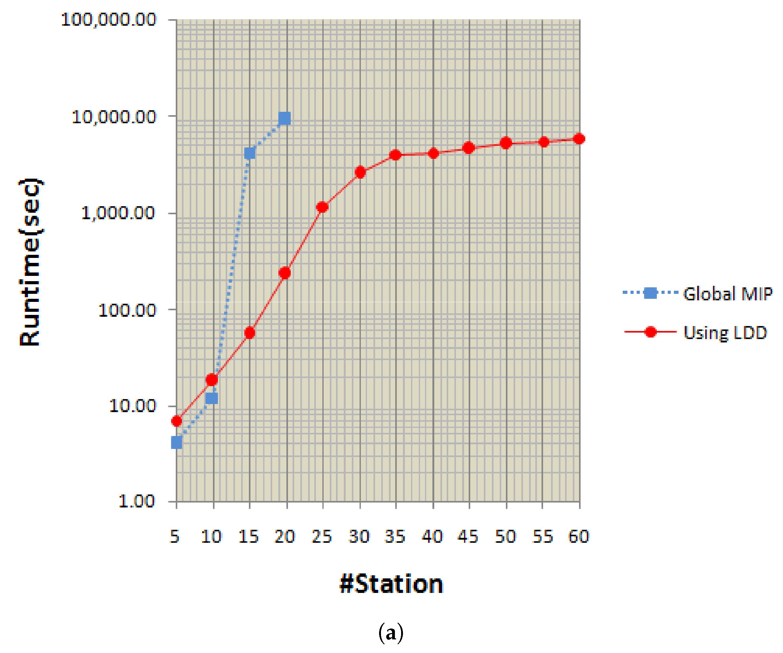
Runtime performance: We compare the runtime performance of the DRRPVT with LDD to DRRPVT with MILP as shown Figure 2a. The x-axis denotes the scale of problem where we vary the number of stations from 5 to 60. The y-axis denotes the total time taken to solve problem in seconds. Except on small instances (e.g., 10 stations), DRRPVT outperforms the MILP with respect to runtime. The MILP is unable to finish within a cutoff time of 3 h for any problem with more than 20 stations, whereas DRRPVT is able to obtain near optimal solutions on problems with 60 stations with less than 3 h. DRRPVT becomes relatively stable after reaching 35 stations (red curve of Figure 2a). It could be easily speeded up by running our approach in a server of higher performance in real-world applications. Meanwhile, we have observed reductions trend in runtime when using main station clustering on problems with 100–200 stations and it scaled in similar trend with respect to using vs. not using main stations.

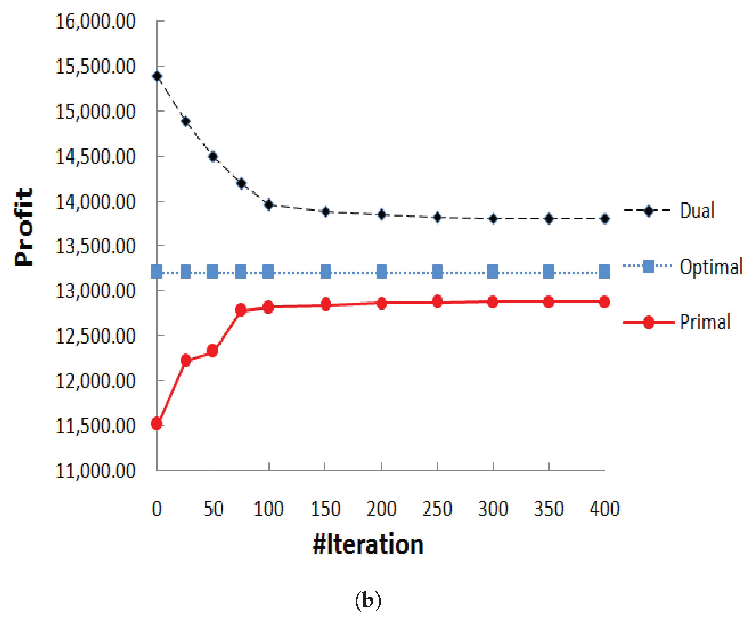
Duality gap: We demonstrate the convergence of LDD to near optimal solutions. LDD achieves an optimal solution if the duality gap, i.e., the gap between primal and dual solutions, becomes zero. Figure 2b show that the duality gap for the instances with 30 stations (grouped into 6 main stations). For these larger problems we are able to obtain a solution with the duality gap of less than 1%.

6.4. Theorem

The maximum total profit $U_s^t$ is achieved if and only if the number of base stations s are five times as likely as the number of main stations $\tilde{s}$, base stations s are twenty times as likely as the number of carrier vehicles, base stations s are three times as likely as the number of bike trailers. At that point, $U_s^t$ achieves the value of maximum.

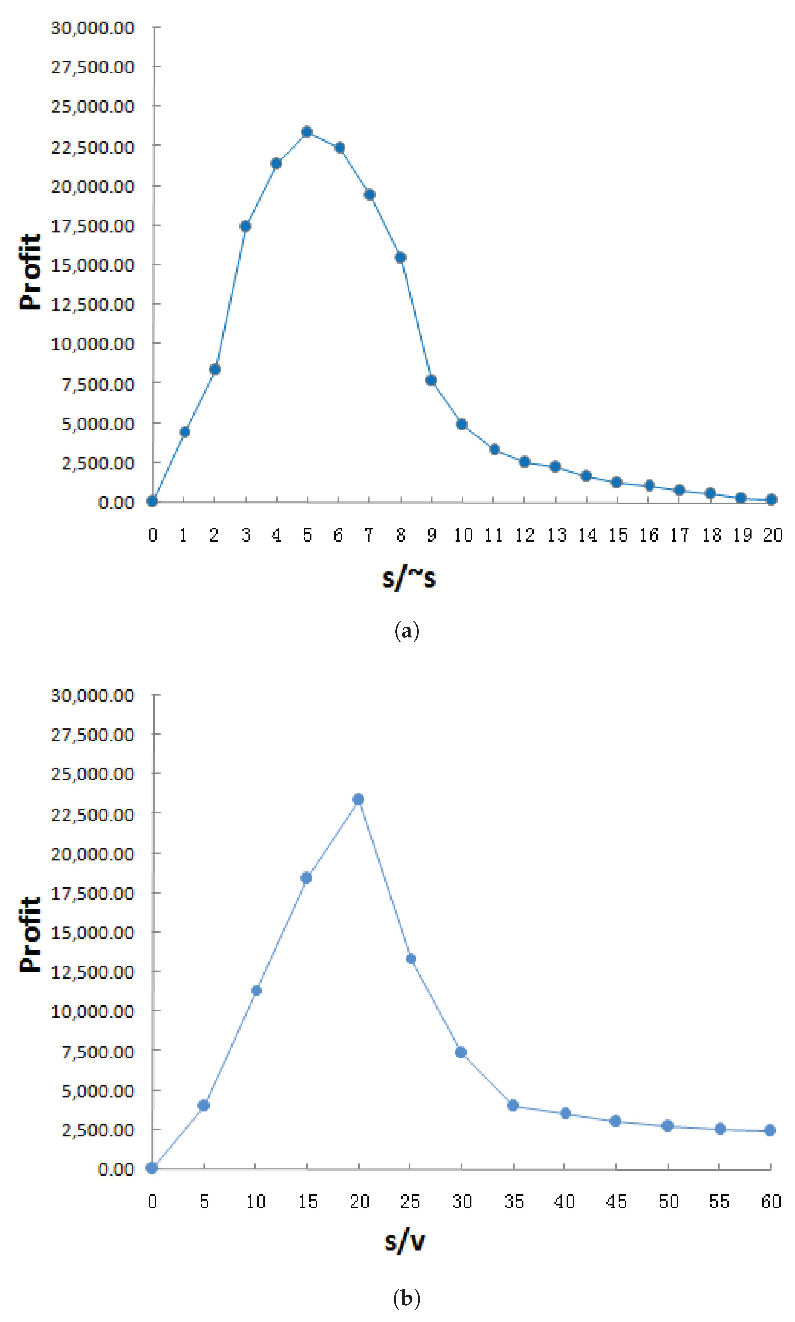
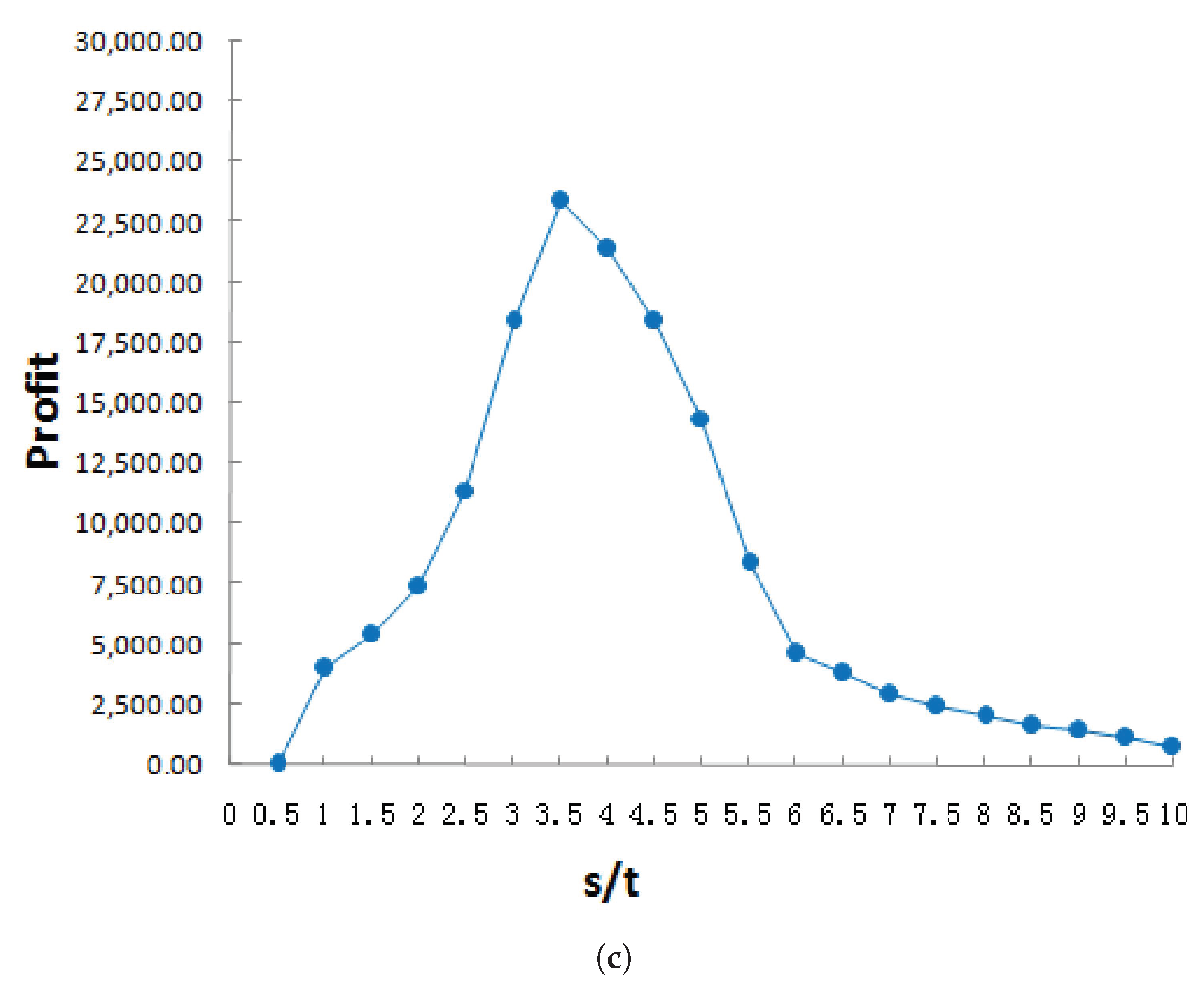
First, we compare the profit of the DRRPVT with the ratio of base stations to main stations in Figure 3a. The x-axis denotes the scale of the ratio from 0 to 60. The y-axis denotes the data of total profit from DRRPVT. The total profit is able to obtain maximum on the ratio with 5. Secondly, we compare the profit of the DRRPVT with the ratio of base stations to vehicles in Figure 3b. The x-axis denotes the scale of the ratio from 0 to 60. The y-axis denotes the data of total profit from DRRPVT. The total profit is able to obtain maximum on the ratio with 20. Finally, we compare the profit of the DRRPVT with the ratio of base stations to trailers in Figure 3c. The x-axis denotes the scale of the ratio from 0 to 60. The y-axis denotes the data of total profit from DRRPVT. The total profit is able to obtain maximum on the ratio with 3.

We obtain: $U=R\times X-\widehat{P}\times f_v(\tilde{s},v)-P\times X\times f_t(s,t)$ where X denotes the actual demand of hired bikes belongs to the poisson distribution.$R,\widehat{P},P$ denote the value of hired bikes, trailer tasks and vehicle tasks are constants. $\tilde{s}$, s, v, t denote the number of main stations, base stations, and vehicles. The theorem is derived from empirical plotting of the profit metric against various system parameters based on the output from LDD method. Therefore, it is based on theoretical characterization of “the optimal” solution in which one gets maximum benefit.

7. Conclusions

We propose an optimization model to jointly consider the usage of carrier vehicles and bike trailers. Additionally, we build a profit objective to calculate the value of carrier vehicle routing and bike trailers, by considering a variety of constraints with respect to vehicle routing and bike repositioning. In the future, we will develop a budget feasible mechanism that solves the uncertainties in completion time of trailer tasks and build an iterative scenario generation approach in which a trailer can pick bikes from one or several stations and then drop them at one or more stations. It is also interesting to investigate the possibility of learning action models [29,30,31,32] and recognizing plans [33,34,35] to help improving bike repositioning under the framework of DRRPVT.

References

1. Tsai, M.; Chen, P.; Hong, Y.J. Enhancing the utilization of public bike sharing systems using return anxiety information. Future Gener. Comp. Syst. 2019, 92, 961–971. [Google Scholar] [CrossRef]
2. Hulot, P.; Aloise, D.; Jena, S.D. Towards Station-Level Demand Prediction for Effective Rebalancing in Bike-Sharing Systems. In Proceedings of the 24th ACM SIGKDD International Conference on Knowledge Discovery & Data Mining 2018, London, UK, 19–23 August 2018; pp. 378–386. [Google Scholar]
3. Lowalekar, M.; Varakantham, P.; Ghosh, S.; Jena, S.D.; Jaillet, P. Online Repositioning in Bike Sharing Systems. In Proceedings of the Twenty-Seventh International Conference on Automated Planning and Scheduling 2017, Pittsburgh, PA, USA, 18–23 June 2017; pp. 200–208. [Google Scholar]
4. Vulcano, G.J.; van Ryzin, G.J.; Ratliff, R. Estimating Primary Demand for Substitutable Products from Sales Transaction Data. Oper. Res. 2012, 60, 313–334. [Google Scholar] [CrossRef] [Green Version]
5. Schuijbroek, J.; Hampshire, R.C.; van Hoeve, W. Inventory rebalancing and vehicle routing in bike sharing systems. Eur. J. Oper. Res. 2017, 257, 992–1004. [Google Scholar] [CrossRef] [Green Version]
6. Shu, J.; Chou, M.C.; Liu, Q.; Teo, C.; Wang, I. Models for Effective Deployment and Redistribution of Bicycles Within Public Bicycle-Sharing Systems. Oper. Res. 2013, 61, 1346–1359. [Google Scholar] [CrossRef]
7. Chen, Q.; Liu, M.; Liu, X. Bike Fleet Allocation Models for Repositioning in Bike-Sharing Systems. IEEE Intell. Transport. Syst. Mag. 2018, 10, 19–29. [Google Scholar] [CrossRef]
8. Ghosh, S.; Varakantham, P.; Adulyasak, Y.; Jaillet, P. Dynamic Repositioning to Reduce Lost Demand in Bike Sharing Systems. J. Artif. Intell. Res. 2017, 58, 387–430. [Google Scholar] [CrossRef]
9. Pfrommer, J.; Warrington, J.; Schildbach, G.; Morari, M. Dynamic Vehicle Redistribution and Online Price Incentives in Shared Mobility Systems. IEEE Trans. Intell. Transp. Syst. 2014, 15, 1567–1578. [Google Scholar] [CrossRef] [Green Version]
10. Ghosh, S.; Varakantham, P. Incentivizing the Use of Bike Trailers for Dynamic Repositioning in Bike Sharing Systems. In Proceedings of the International Conference on Automated Planning and Scheduling 2017, Pittsburgh, PA, USA, 18–23 June 2017; pp. 373–381. [Google Scholar]
11. Ghosh, S.; Trick, M.; Varakantham, P. Robust Repositioning to Counter Unpredictable Demand in Bike Sharing Systems. In Proceedings of the International Joint Conference on Artificial Intelligence, New York, NY, USA, 9–15 July 2016; pp. 3096–3102. [Google Scholar]
12. Ruffieux, S.; Mugellini, E.; Khaled, O.A. Predictive Modeling for Optimization of Field Operations in Bike-Sharing Systems. In Proceedings of the 6th Swiss Conference on Data Science, SDS 2019, Bern, Switzerland, 14 June 2019; pp. 119–124. [Google Scholar] [CrossRef] [Green Version]
13. Liu, J.; Sun, L.; Chen, W.; Xiong, H. Rebalancing Bike Sharing Systems: A Multi-source Data Smart Optimization. In Proceedings of the 22nd ACM SIGKDD International Conference on Knowledge Discovery and Data Mining, San Francisco, CA, USA, 13–17 August 2016; pp. 1005–1014. [Google Scholar] [CrossRef]
14. Ghosh, S.; Koh, J.Y.; Jaillet, P. Improving Customer Satisfaction in Bike Sharing Systems through Dynamic Repositioning. In Proceedings of the International Joint Conference on Artificial Intelligence, Macao, China, 14–16 August 2019; pp. 5864–5870. [Google Scholar]
15. Liu, Z.; Yu, H.; Wang, L.; Hu, L.; Yang, Q. Ethically Aligned Mobilization of Community Effort to Reposition Shared Bikes. In Proceedings of the AAAI, Honolulu, HI, USA, 14 June 2019. [Google Scholar]
16. Lin, J.; Yang, T.; Chang, Y. A hub location inventory model for bicycle sharing system design: Formulation and solution. Comput. Ind. Eng. 2013, 65, 77–86. [Google Scholar] [CrossRef]
17. Chemla, D.; Meunier, F.; Calvo, R.W. Bike sharing systems: Solving the static rebalancing problem. Discret. Optim. 2013, 10, 120–146. [Google Scholar] [CrossRef]
18. Gaspero, L.D.; Rendl, A.; Urli, T. Balancing bike sharing systems with constraint programming. Constraints 2016, 21, 318–348. [Google Scholar] [CrossRef]
19. Wang, N.; Zgaya, H.; Mathieu, P.; Hammadi, S. An Agent-Based Distributed Approach for Bike Sharing Systems. In Proceedings of the ICCS, Cambridge, MA, USA, 22–27 July 2018; pp. 540–552. [Google Scholar]
20. Singla, A.; Santoni, M.; Bartók, G.; Mukerji, P.; Meenen, M.; Krause, A. Incentivizing Users for Balancing Bike Sharing Systems. In Proceedings of the AAAI, Austin, TX, USA, 25–30 January 2015; pp. 723–729. [Google Scholar]
21. Liu, Z.; Yu, H.; Wang, L.; Hu, L.; Yang, Q. Social Mobilization to Reposition Indiscriminately Parked Shareable Bikes. In Proceedings of the AAMAS, Montreal, QC, Canada, 13–17 May 2019; pp. 2099–2101. [Google Scholar]
22. Hartuv, E.; Agmon, N.; Kraus, S. Scheduling Spare Drones for Persistent Task Performance under Energy Constraints. In Proceedings of the AAMAS, Stockholm, Sweden, 10–15 July 2018; pp. 532–540. [Google Scholar]
23. Zhang, R.; Pavone, M. Control of Robotic Mobility-On-Demand Systems: A Queueing-Theoretical Perspective. Int. J. Robot. Res. 2016, 35, 186–203. [Google Scholar] [CrossRef]
24. Ghosh, S.; Varakantham, P. Dispatch Guided Allocation Optimization for Effective Emergency Response. In Proceedings of the AAAI, New Orleans, LA, USA, 2–7 February 2018; pp. 775–783. [Google Scholar]
25. Konda, M.; Ghosh, S.; Varakantham, P. Reserved Optimisation: Handling Incident Priorities in Emergency Response Systems. In Proceedings of the ICAPS, Delft, The Netherlands, 24–29 June 2018; pp. 330–338. [Google Scholar]
26. Jha, S.S.; Cheng, S.; Lowalekar, M.; Wong, N.; Rajendram, R.; Tran, T.K.; Varakantham, P.; Truong, T.N.; Rahman, F.B.A. Upping the Game of Taxi Driving in the Age of Uber. In Proceedings of the AAAI, New Orleans, LA, USA, 2–7 February 2018; pp. 7779–7785. [Google Scholar]
27. Cavallo, R. Mechanism design for dynamic settings. SIGecom Exch. 2009, 8, 7. [Google Scholar] [CrossRef] [Green Version]
28. Do, L.; Lauw, H.W.; Wang, K. Mining Revenue-Maximizing Bundling Configuration. Proc. VLDB Endow. 2015, 8, 593–604. [Google Scholar] [CrossRef]
29. Zhuo, H.H.; Yang, Q. Action-model acquisition for planning via transfer learning. Artif. Intell. 2014, 212, 80–103. [Google Scholar] [CrossRef]
30. Zhuo, H.H.; Kambhampati, S. Model-lite planning: Case-based vs. model-based approaches. Artif. Intell. 2014, 246, 1–21. [Google Scholar] [CrossRef] [Green Version]
31. Zhuo, H.H.; Muñoz-Avila, H.; Yang, Q. Learning hierarchical task network domains from partially observed plan traces. Artif. Intell. 2014, 212, 134–157. [Google Scholar] [CrossRef]
32. Zhuo, H.H.; Zha, Y.; Kambhampati, S. Discovering Underlying Plans Based on Shallow Models. ACM Trans. Intell. Syst. Technol. 2020, 11, 18:1–18:30. [Google Scholar] [CrossRef] [Green Version]
33. Zhuo, H.H. Human-Aware Plan Recognition. In Proceedings of the AAAI Conference on Artificial Intelligence, San Francisco, CA, USA, 4–9 February 2017; pp. 3686–3693. [Google Scholar]
34. Zhuo, H.H. Recognizing Multi-Agent Plans When Action Models and Team Plans Are Both Incomplete. ACM Trans. Intell. Syst. Technol. 2019, 10, 30:1–30:24. [Google Scholar] [CrossRef]
35. Feng, W.; Zhuo, H.H.; Kambhampati, S. Extracting Action Sequences from Texts Based on Deep Reinforcement Learning. In Proceedings of the International Joint Conferences on Artifical Intelligence (IJCAI), Stockholm, Sweden, 13–19 July 2018; pp. 4064–4070. [Google Scholar]
Figure 1. Correlation of demand and supply: (a) DRRPV, (b) DRRPT, and (c) DRRPVT.
Applsci 11 07227 g001
Figure 2. (a) Runtime comparison between the global MILP and LDD, (b) Duality gap in the synthetic data set with 30 stations.
Applsci 11 07227 g002aApplsci 11 07227 g002b
Figure 3. The maximal profit of the DRRPVT with the ratio of base stations to: (a) main stations, (b) vehicles, and (c) trailers.
Applsci 11 07227 g003aApplsci 11 07227 g003b