
Evaluation of Machine Learning Predictions of a Highly Resolved Time Series of Chlorophyll-a Concentration

 , and
, and
Abstract
:1. Introduction
2. Materials and Methods
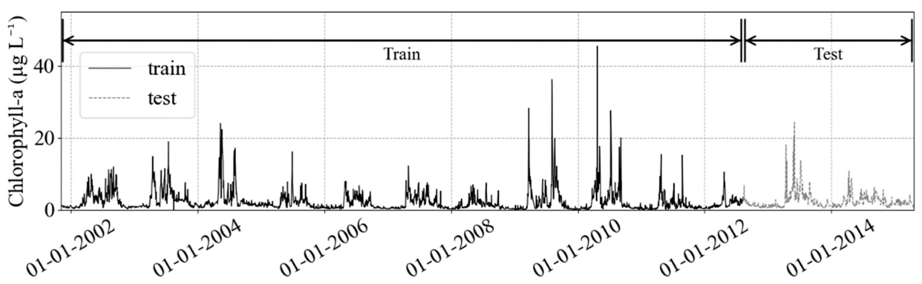
2.1. Datasets
2.2. Data Preprocessing
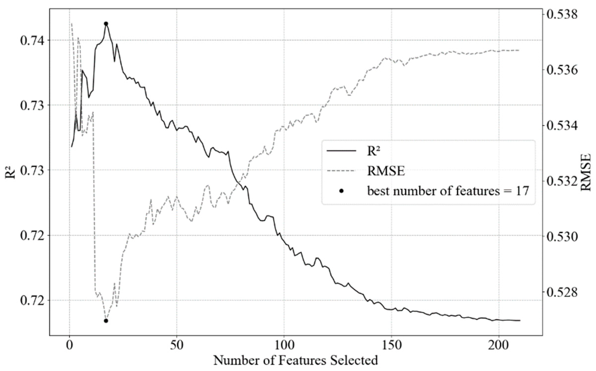
2.3. Feature Engineering and Selection
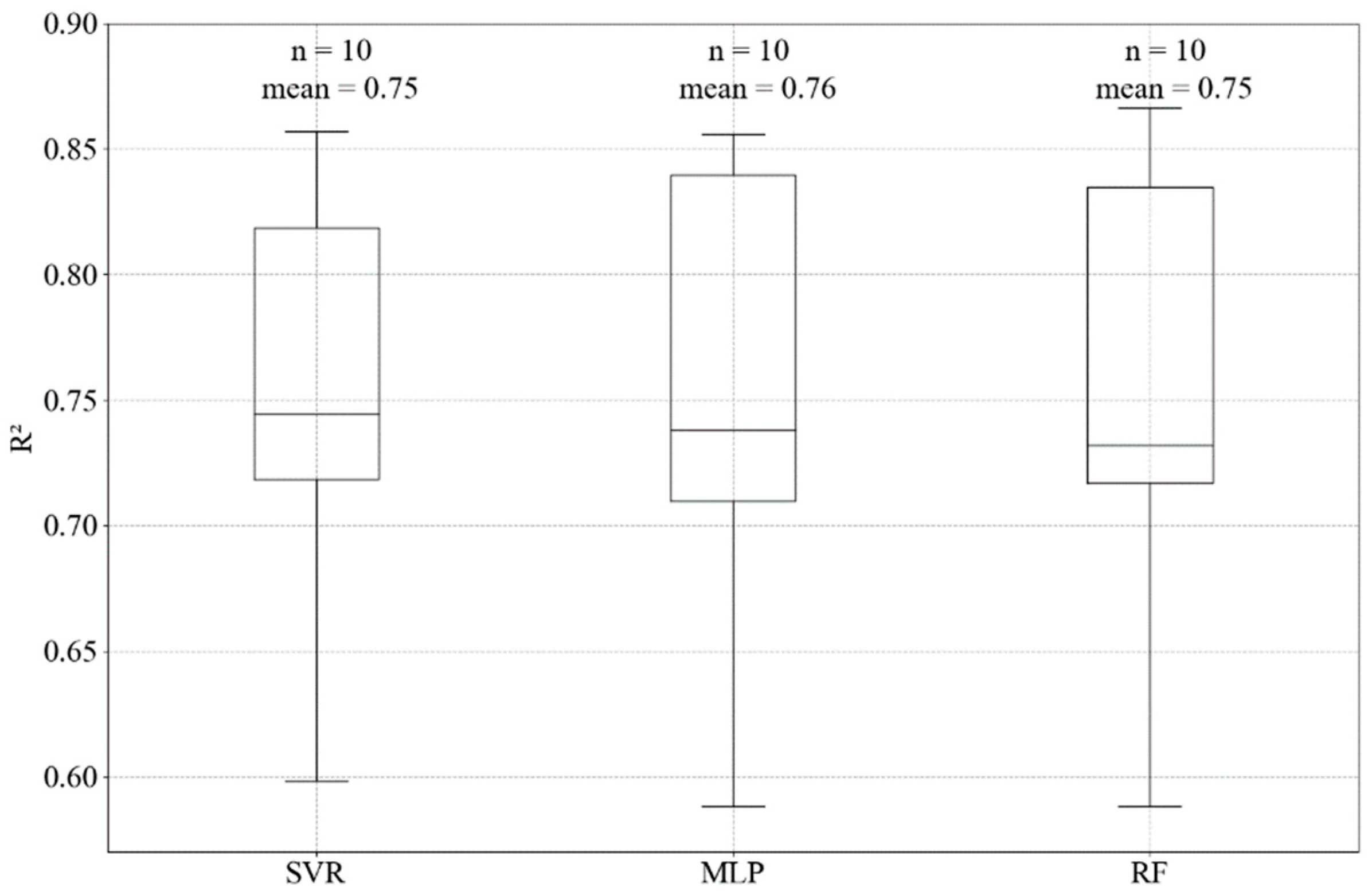
2.4. Model Selection and Hyperparameter Tuning
2.5. SARIMA Model
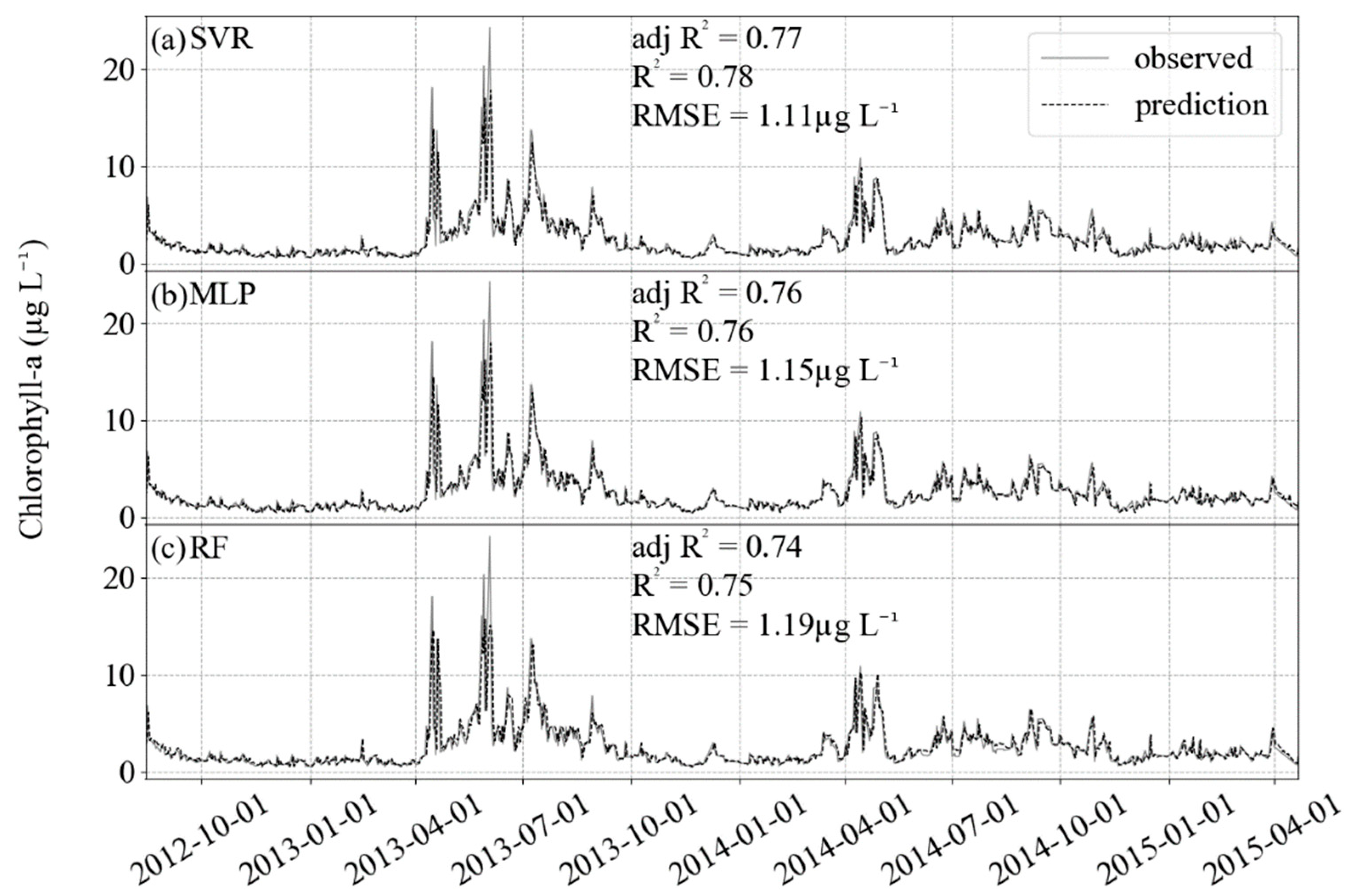
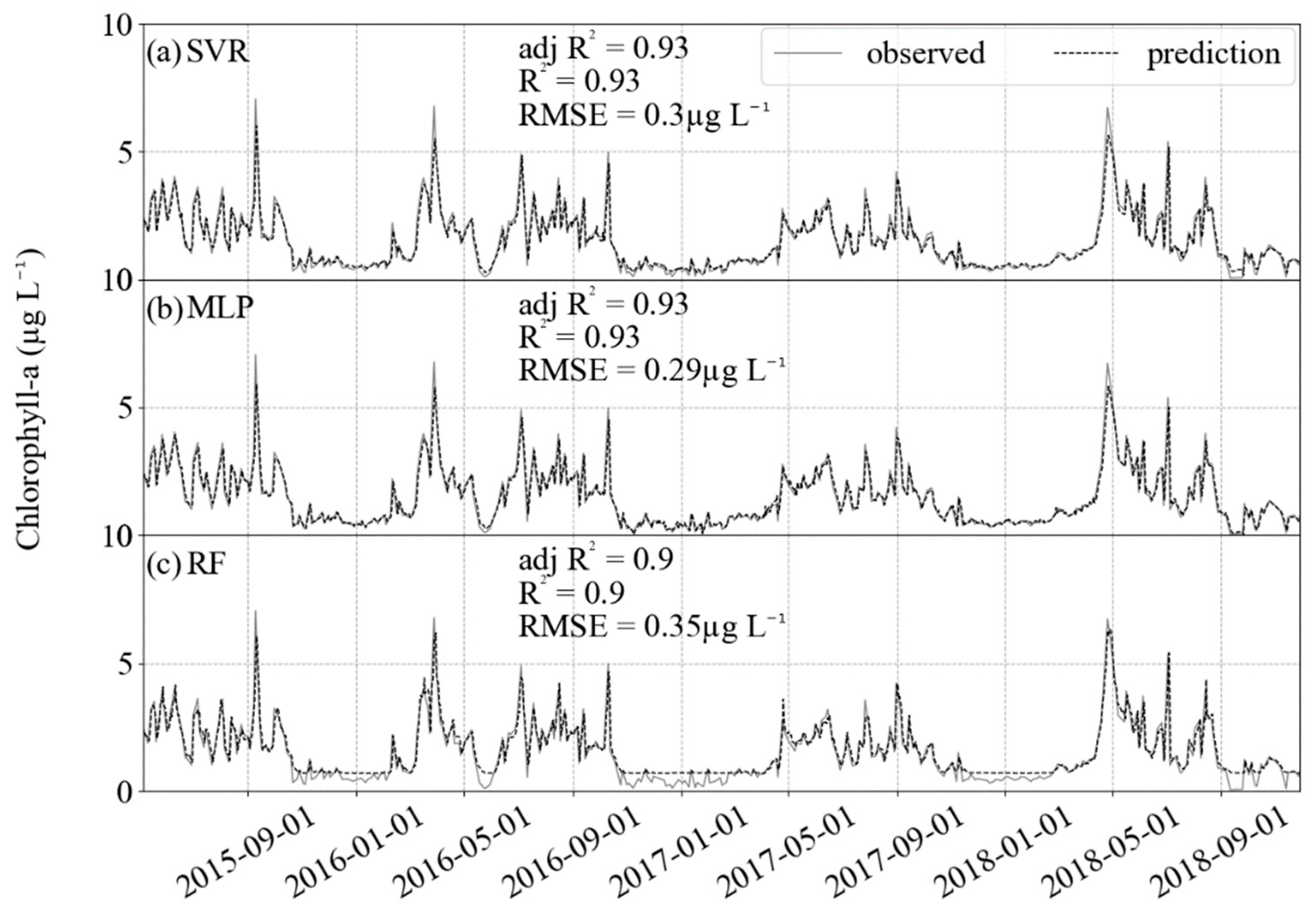
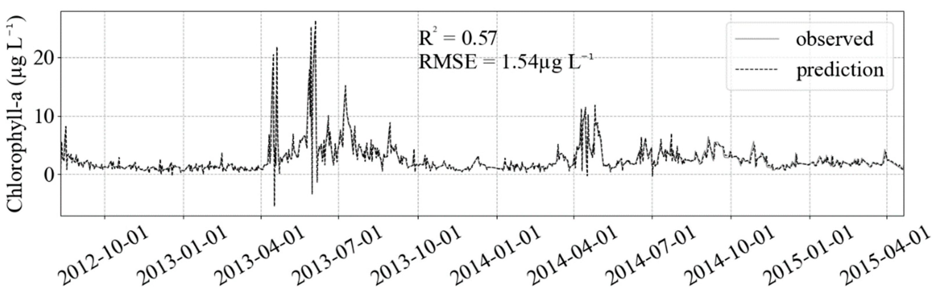
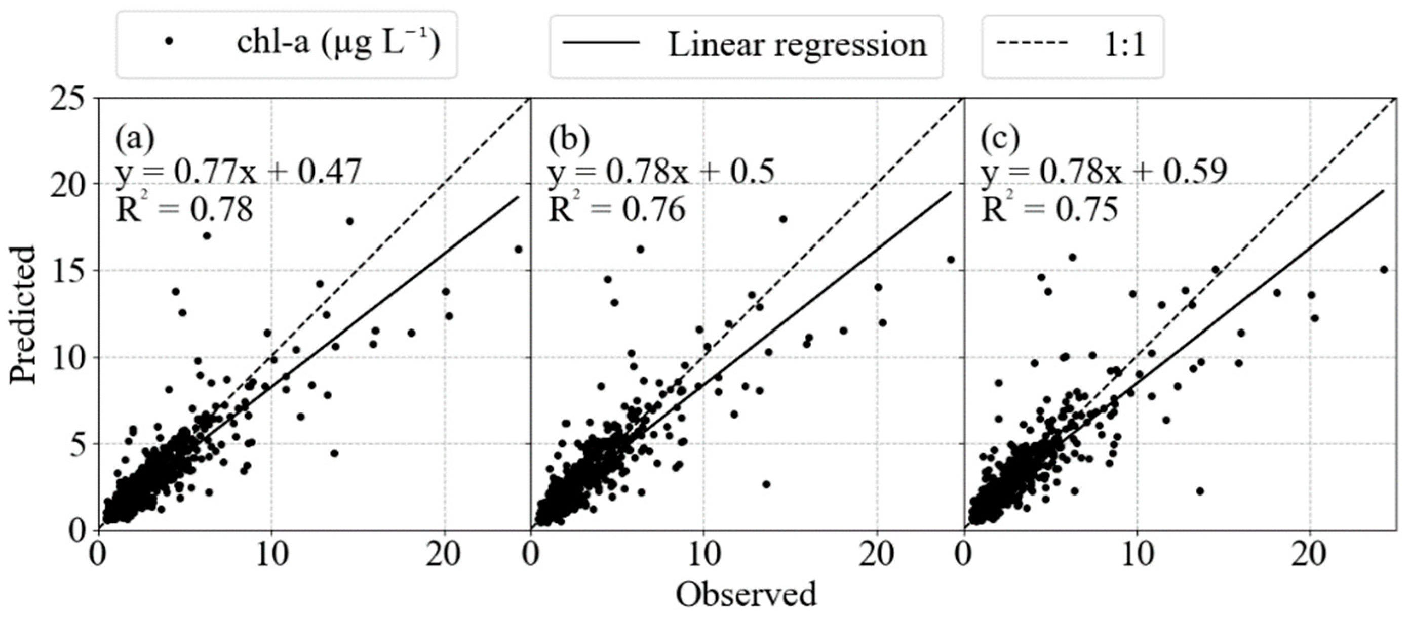
3. Results
4. Discussion
5. Conclusions
Supplementary Materials
Author Contributions
Funding
Institutional Review Board Statement
Informed Consent Statement
Data Availability Statement
Acknowledgments
Conflicts of Interest
References
- Huot, Y.; Babin, M.; Bruyant, F.; Grob, C.; Twardowski, M.S.; Claustre, H. Does chlorophyll a provide the best index of phytoplankton biomass for primary productivity studies? Biogeosciences 2007, 4, 853–868. [Google Scholar] [CrossRef] [Green Version]
- Terauchi, G.; Tsujimoto, R.; Ishizaka, J.; Nakata, H. Preliminary assessment of eutrophication by remotely sensed chlorophyll-a in Toyama Bay, the Sea of Japan. J. Oceanogr. 2014, 70, 175–184. [Google Scholar] [CrossRef]
- Luo, W.; Zhu, S.; Wu, S.; Dai, J. Comparing artificial intelligence techniques for chlorophyll-a prediction in US lakes. Environ. Sci. Pollut. Res. 2019, 26, 30524–30532. [Google Scholar] [CrossRef]
- Botkin, D.B.; Saxe, H.; Araujo, M.B.; Betts, R.; Bradshaw, R.H.; Cedhagen, T.; Chesson, P.; Dawson, T.P.; Etterson, J.R.; Faith, D.P. Forecasting the effects of global warming on biodiversity. BioScience 2007, 57, 227–236. [Google Scholar] [CrossRef]
- Shamshirband, S.; Jafari Nodoushan, E.; Adolf, J.E.; Abdul Manaf, A.; Mosavi, A.; Chau, K.W. Ensemble models with uncertainty analysis for multi-day ahead forecasting of chlorophyll a concentration in coastal waters. Eng. Appl. Comput. Fluid Mech. 2019, 13, 91–101. [Google Scholar] [CrossRef] [Green Version]
- Shin, Y.; Kim, T.; Hong, S.; Lee, S.; Kim, T.; Park, M.S.; Park, J.; Heo, T.-Y. Prediction of Chlorophyll-a Concentrations in the Nakdong River Using Machine Learning Methods. Water 2020, 12, 1822. [Google Scholar] [CrossRef]
- Kwiatkowska, E.J.; Fargion, G.S. Application of machine-learning techniques toward the creation of a consistent and calibrated global chlorophyll concentration baseline dataset using remotely sensed ocean color data. IEEE Trans. Geosci. Remote Sens. 2003, 41, 2844–2860. [Google Scholar] [CrossRef]
- Cho, H.; Choi, U.J.; Park, H. Deep Learning Application to Time Series Prediction of Daily Chlorophyll-a Concentration. WIT Trans. Ecol. Environ. 2018, 215, 157–163. [Google Scholar] [CrossRef] [Green Version]
- Krasnopolsky, V.; Nadiga, S.; Mehra, A.; Bayler, E. Adjusting Neural Network to a Particular Problem: Neural Network-Based Empirical Biological Model for Chlorophyll Concentration in the Upper Ocean. Appl. Comput. Intell. Soft Comput. 2018, 2018, 7057363. [Google Scholar] [CrossRef]
- Keller, S.; Maier, P.M.; Riese, F.M.; Norra, S.; Holbach, A.; Börsig, N.; Wilhelms, A.; Moldaenke, C.; Zaake, A.; Hinz, S. Hyperspectral Data and Machine Learning for Estimating CDOM, Chlorophyll a, Diatoms, Green Algae and Turbidity. Int. J. Environ. Res. Public Health 2018, 15, 1881. [Google Scholar] [CrossRef] [Green Version]
- Liu, X.; Feng, J.; Wang, Y. Chlorophyll a predictability and relative importance of factors governing lake phytoplankton at different timescales. Sci. Total Environ. 2019, 648, 472–480. [Google Scholar] [CrossRef] [PubMed]
- Lo, A.W.; Siah, K.W.; Wong, C.H. Machine learning with statistical imputation for predicting drug approvals. Harv. Data Sci. Rev. 2019, 1, 1. [Google Scholar] [CrossRef]
- Brownlee, J. How to Develop Multivariate Multi-Step Time Series Forecasting Models for Air Pollution. Machine Learning Mastery. Available online: https://machinelearningmastery.com/how-to-develop-machine-learning-models-for-multivariate-multi-step-air-pollution-time-series-forecasting/ (accessed on 24 July 2020).
- Park, Y.; Cho, K.H.; Park, J.; Cha, S.M.; Kim, J.H. Development of early-warning protocol for predicting chlorophyll-a concentration using machine learning models in freshwater and estuarine reservoirs, Korea. Sci. Total Environ. 2015, 502, 31–41. [Google Scholar] [CrossRef]
- Box, G.; Jenkins, G. Time Series Analysis Forecasting and Control, rev. ed.; Holden-Day: Oakland, CA, USA, 1976; pp. 303–305. [Google Scholar]
- Pedregosa, F.; Varoquaux, G.; Gramfort, A.; Michel, V.; Thirion, B.; Grisel, O.; Blondel, M.; Prettenhofer, P.; Weiss, R.; Dubourg, V.; et al. Scikit-Learn: Machine Learning in Python. J. Mach. Learn. Res. 2011, 12, 2826–2830. [Google Scholar] [CrossRef]
- Buitinck, L.; Louppe, G.; Blondel, M.; Pedregosa, F.; Mueller, A.; Grisel, O.; Niculae, V.; Prettenhofer, P.; Gramfort, A.; Grobler, J.; et al. API design for machine learning software: Experiences from the scikit-learn project. In Proceedings of the ECML PKDD Workshop: Languages for Data Mining and Machine Learning, Prage, Czech Republic, 23–27 September 2013; pp. 108–122. [Google Scholar]
- McKinney, W.; Perktold, J.; Seabold, S. Time Series Analysis in Python with Statsmodels. In Proceedings of the 10th Python in Science Conference, Austin, TX, USA, 11−16 July 2011; Walt, S., van der Millman, J., Eds.; Scipy: Austin, TX, USA, 2011; pp. 107–113. [Google Scholar] [CrossRef] [Green Version]
- Lemenkova, P. Processing Oceanographic Data by Python Libraries Numpy, Scipy and Pandas. Aquat. Res. 2019, 2, 73–91. [Google Scholar] [CrossRef]
- Wiltshire, K.H.; Dürselen, C.-D. Revision and Quality Analyses of the Helgoland Reede Long-Term Phytoplankton Data Archive. Helgol. Mar. Res. 2004, 58, 252–268. [Google Scholar] [CrossRef] [Green Version]
- Beutler, M.; Wiltshire, K.H.; Meyer, B.; Moldaenke, C.; Lüring, C.; Meyerhöfer, M.; Hansen, U.-P.; Dau, H. A fluorometric method for the differentiation of algal populations in vivo and in situ. Photosynth. Res. 2002, 72, 39–53. [Google Scholar] [CrossRef]
- Wiltshire, K.H.; Malzahn, A.M.; Wirtz, K.; Greve, W.; Janisch, S.; Mangelsdorf, P.; Manly, B.F.J.; Boersma, M. Resilience of North Sea Phytoplankton Spring Bloom Dynamics: An Analysis of Long-Term Data at Helgoland Roads. Limnol. Oceanogr. 2008, 53, 1294–1302. [Google Scholar] [CrossRef] [Green Version]
- Raabe, T.; Wiltshire, K.H. Quality Control and Analyses of the Long-Term Nutrient Data from Helgoland Roads, North Sea. J. Sea Res. 2009, 61, 3–16. [Google Scholar] [CrossRef]
- Deutsche Wetterdienst (DWD) Climate Data Center (CDC). Daily Station Observations of Sunshine Duration in Hours for Germany. 2020. Available online: https://cdc.dwd.de/portal/ (accessed on 26 April 2020).
- Deutsche Wetterdienst (DWD) Climate Data Center (CDC). Hourly Mean of Station Observations of Wind Speed ca. 10 m above Ground in m/s for Germany. Available online: https://cdc.dwd.de/portal/ (accessed on 6 February 2020).
- Deutsche Wetterdienst (DWD) Climate Data Center (CDC). Hourly Station Observations of Wind Direction 10 m above Ground in Degree for Germany. Available online: https://cdc.dwd.de/portal/ (accessed on 6 February 2020).
- Greve, W.; Reiners, F.; Nast, J.; Hoffmann, S. Helgoland Roads Meso- and Macrozooplankton Time-Series 1974 to 2004: Lessons from 30 Years of Single Spot, High Frequency Sampling at the Only off-Shore Island of the North Sea. Helgol. Mar. Res. 2004, 58, 274–288. [Google Scholar] [CrossRef] [Green Version]
- Irwin, A.J.; Finkel, Z.V. Mining a Sea of Data: Deducing the Environmental Controls of Ocean Chlorophyll. PLoS ONE 2008, 3, e3836. [Google Scholar] [CrossRef] [PubMed]
- Capuzzo, E.; Lynam, C.P.; Barry, J.; Stephens, D.; Forster, R.M.; Greenwood, N.; McQuatters-Gollop, A.; Silva, T.; van Leeuwen, S.M.; Engelhard, G.H. A Decline in Primary Production in the North Sea over 25 Years, Associated with Reductions in Zooplankton Abundance and Fish Stock Recruitment. Glob. Chang. Biol. 2018, 24, e352–e364. [Google Scholar] [CrossRef] [PubMed]
- Scharfe, M.; Wiltshire, K.H. Modeling of Intra-Annual Abundance Distributions: Constancy and Variation in the Phenology of Marine Phytoplankton Species over Five Decades at Helgoland Roads (North Sea). Ecol. Model. 2019, 404, 46–60. [Google Scholar] [CrossRef]
- Mao, H.; Meng, J.; Ji, F.; Zhang, Q.; Fang, H. Comparison of Machine Learning Regression Algorithms for Cotton Leaf Area Index Retrieval Using Sentinel-2 Spectral Bands. Appl. Sci. 2019, 9, 1459. [Google Scholar] [CrossRef] [Green Version]
- Tsai, C.-F.; Hsiao, Y.-C. Combining Multiple Feature Selection Methods for Stock Prediction: Union, Intersection, and Multi-Intersection Approaches. Decis. Support. Syst. 2010, 50, 258–269. [Google Scholar] [CrossRef]
- Lee, J.; Wang, W.; Harrou, F.; Sun, Y. Wind Power Prediction Using Ensemble Learning-Based Models. IEEE Access 2020, 8, 61517–61527. [Google Scholar] [CrossRef]
- Saberioon, M.; Brom, J.; Nedbal, V.; Souček, P.; Císař, P. Chlorophyll-a and Total Suspended Solids Retrieval and Mapping Using Sentinel-2A and Machine Learning for Inland Waters. Ecol. Indic. 2020, 113, 106236. [Google Scholar] [CrossRef]
- Tang, W.; Li, Z.; Cassar, N. Machine Learning Estimates of Global Marine Nitrogen Fixation. J. Geophys. Res. Biogeosci. 2019, 124, 717–730. [Google Scholar] [CrossRef]
- Lenert, M.C.; Walsh, C.G. Balancing Performance and Interpretability: Selecting Features with Bootstrapped Ridge Regression. AMIA Annu. Symp. Proc. 2018, 2018, 1377–1386. [Google Scholar]
- Breiman, L. Random forests. Mach. Learn. 2001, 45, 5–32. [Google Scholar] [CrossRef] [Green Version]
- Cortes, C.; Vapnik, V. Support-Vector Networks. Mach. Learn. 1995, 20, 273–297. [Google Scholar] [CrossRef]
- Hornik, K.; Stinchcombe, M.; White, H. Multilayer Feedforward Networks Are Universal Approximators. Neural Netw. 1989, 2, 359–366. [Google Scholar] [CrossRef]
- Gardner, M.W.; Dorling, S.R. Artificial Neural Networks (the Multilayer Perceptron)—A Review of Applications in the Atmospheric Sciences. Atmos. Environ. 1998, 32, 2627–2636. [Google Scholar] [CrossRef]
- Phung, V.H.; Rhee, E.J. A High-Accuracy Model Average Ensemble of Convolutional Neural Networks for Classification of Cloud Image Patches on Small Datasets. Appl. Sci. 2019, 9, 4500. [Google Scholar] [CrossRef] [Green Version]
- Ooi, K.S.; Chen, Z.; Poh, P.E.; Cui, J. BOD5 Prediction Using Machine Learning Methods. Water Supply 2021, ws2021202. [Google Scholar] [CrossRef]
- Sun, Y.; Li, J.; Liu, J.; Chow, C.; Sun, B.; Wang, R. Using Causal Discovery for Feature Selection in Multivariate Numerical Time Series. Mach. Learn. 2015, 101, 377–395. [Google Scholar] [CrossRef]
- Lee, S.; Chung, J.Y. The Machine Learning-Based Dropout Early Warning System for Improving the Performance of Dropout Prediction. Appl. Sci. 2019, 9, 3093. [Google Scholar] [CrossRef] [Green Version]
- Rezaie-Balf, M.; Kisi, O.; Chua, L.H.C. Application of Ensemble Empirical Mode Decomposition Based on Machine Learning Methodologies in Forecasting Monthly Pan Evaporation. Hydrol. Res. 2019, 50, 498–516. [Google Scholar] [CrossRef]
- Schloen, J.; Stanev, E.V.; Grashorn, S. Wave-Current Interactions in the Southern North Sea: The Impact on Salinity. Ocean. Model. 2017, 111, 19–37. [Google Scholar] [CrossRef]
- Chen, W.-H.; Hsu, S.-H.; Shen, H.-P. Application of SVM and ANN for Intrusion Detection. Comput. Oper. Res. 2005, 32, 2617–2634. [Google Scholar] [CrossRef]
- Munson, M.A.; Caruana, R. On Feature Selection, Bias-Variance, and Bagging. In Machine Learning and Knowledge Discovery in Databases; Buntine, W., Grobelnik, M., Mladenić, D., Shawe-Taylor, J., Eds.; Lecture Notes in Computer Science; Springer: Berlin/Heidelberg, Germany, 2009; Volume 5782, pp. 144–159. ISBN 978-3-642-04173-0. [Google Scholar]
- Blauw, A.N.; Benincà, E.; Laane, R.W.P.M.; Greenwood, N.; Huisman, J. Predictability and Environmental Drivers of Chlorophyll Fluctuations Vary across Different Time Scales and Regions of the North Sea. Progress Oceanogr. 2018, 161, 1–18. [Google Scholar] [CrossRef]


| Parameters | Units | Counts | Mean | Std | Min | Max | Median |
|---|---|---|---|---|---|---|---|
| Secchi depth | m | 4920 | 3.70 | 1.80 | 0.20 | 12.00 | 3.67 |
| SST | °C | 4920 | 10.64 | 5.00 | 1.10 | 20.00 | 10.30 |
| Salinity | _ | 4920 | 32.31 | 1.06 | 26.71 | 36.11 | 32.42 |
| SiO4 | µmol L−1 | 4920 | 6.49 | 5.04 | 0.01 | 37.20 | 5.26 |
| PO4 | µmol L−1 | 4920 | 0.56 | 0.41 | 0.01 | 3.98 | 0.53 |
| NO3 | µmol L−1 | 4920 | 10.19 | 9.82 | 0.10 | 77.38 | 7.12 |
| Sunlight Duration | h | 4920 | 4.78 | 4.52 | 0.00 | 16.60 | 3.60 |
| NAO index | _ | 4920 | −9.44 | 121.55 | −564.29 | 351.95 | −0.52 |
| Wind Direction | Degrees [°] | 4920 | 203.09 | 74.71 | 20.00 | 353.00 | 212.00 |
| Wind Speed | m s−1 | 4920 | 8.23 | 3.28 | 1.60 | 20.80 | 7.80 |
| Zooplankton Abundance | individuals m−3 | 4920 | 3164.70 | 4450.64 | 5.00 | 75,364.50 | 1676.21 |
| Chlorophyll-a | µg m−1 | 4920 | 2.40 | 2.86 | 0.00 | 45.45 | 1.48 |
| Predictors | Code | Correlation |
|---|---|---|
| year | year | −0.05 |
| sin (days) | sin (days) | 0.04 |
| cos (days) | cos (days) | −0.46 |
| Secchi depth | SD | 0.15 |
| Sea Surface Temperature | SST | 0.27 |
| Salinity | Salinity | −0.22 |
| Silicate | SiO4 | −0.31 |
| Phosphate | PO4 | −0.29 |
| Nitrate | NO3 | −0.09 |
| Sunlight duration | Sunlight | 0.31 |
| NAO index | NAO | 0.06 |
| sin (wind direction) | sin | 0.02 |
| cos (wind direction) | cos | 0.10 |
| Wind Speed | Speed | −0.20 |
| Zooplankton Abundance | Abundance | 0.22 |
| Chlorophyll-a | Chl | 1.00 |
| Features |
|---|
| SD |
| SST |
| Salinity |
| Secchi_−1 |
| SST_−1 |
| SST_−2 |
| SST_−9 |
| SST_−12 |
| SST_−13 |
| SST_−14 |
| SST_−15 |
| Salinity_−1 |
| Chl_−1 |
| Chl_−4 |
| Chl_−5 |
| Chl_−7 |
| Chl_−8 |
| Model | Hyperparameter | Selected Value | Default |
|---|---|---|---|
| SVR | kernel | rbf | rbf |
| C | 3 | 1 | |
| gamma | 0.01 | 0.1 | |
| Epsilon | 0.1 | 0.0001 | |
| MLP | max_iter | 90 | 200 |
| hidden_layer_sizes | 80 | 100 | |
| activation | logistic | relu | |
| solver | adam | adam | |
| Alpha | 0.5 | 0.0001 | |
| warm_start | True | False | |
| RF | bootstrap | True | True |
| max_depth | 11 | None | |
| max_features | 14 | auto | |
| min_samples_leaf | 13 | 1 | |
| min_samples_split | 2 | 2 | |
| n_estimators | 100 | 100 |
| Default | ||||||
| Train | Test | |||||
| adj R2 | R2 | RMSE (µg L−1) | adj R2 | R2 | RMSE (µg L−1) | |
| SVR | 0.81 | 0.82 | 1.255 | 0.63 | 0.71 | 1.273 |
| RF | 0.96 | 0.96 | 0.23 | 0.15 | 0.33 | 1.929 |
| MLP | 1 | 1 | 0.04 | 0.02 | 0.23 | 2.068 |
| Optimized | ||||||
| Train | Test | |||||
| adj R2 | R2 | RMSE (µg L−1) | adj R2 | R2 | RMSE (µg L−1) | |
| SVR | 0.77 | 0.77 | 1.424 | 0.77 | 0.78 | 1.113 |
| RF | 0.81 | 0.81 | 0.495 | 0.74 | 0.75 | 1.189 |
| MLP | 0.75 | 0.75 | 0.56 | 0.76 | 0.76 | 1.144 |
| Linear (Base Model) | ||||||
| Train | Test | |||||
| adj R2 | R2 | RMSE (µg L−1) | adj R2 | R2 | RMSE (µg L−1) | |
| 0.74 | 0.76 | 1.47 | 0.65 | 0.73 | 1.227 | |
Publisher’s Note: MDPI stays neutral with regard to jurisdictional claims in published maps and institutional affiliations. |
© 2021 by the authors. Licensee MDPI, Basel, Switzerland. This article is an open access article distributed under the terms and conditions of the Creative Commons Attribution (CC BY) license (https://creativecommons.org/licenses/by/4.0/).
Share and Cite
Amorim, F.d.L.L.d.; Rick, J.; Lohmann, G.; Wiltshire, K.H. Evaluation of Machine Learning Predictions of a Highly Resolved Time Series of Chlorophyll-a Concentration. Appl. Sci. 2021, 11, 7208. https://doi.org/10.3390/app11167208
Amorim FdLLd, Rick J, Lohmann G, Wiltshire KH. Evaluation of Machine Learning Predictions of a Highly Resolved Time Series of Chlorophyll-a Concentration. Applied Sciences. 2021; 11(16):7208. https://doi.org/10.3390/app11167208
Chicago/Turabian StyleAmorim, Felipe de Luca Lopes de, Johannes Rick, Gerrit Lohmann, and Karen Helen Wiltshire. 2021. "Evaluation of Machine Learning Predictions of a Highly Resolved Time Series of Chlorophyll-a Concentration" Applied Sciences 11, no. 16: 7208. https://doi.org/10.3390/app11167208
APA StyleAmorim, F. d. L. L. d., Rick, J., Lohmann, G., & Wiltshire, K. H. (2021). Evaluation of Machine Learning Predictions of a Highly Resolved Time Series of Chlorophyll-a Concentration. Applied Sciences, 11(16), 7208. https://doi.org/10.3390/app11167208