Approaches to Numerical Solution of Optimal Control Problem Using Evolutionary Computations

Abstract

Two approaches to the numerical solution of the optimal control problem are studied. The direct approach is based on the reduction of the optimal control problem to a nonlinear programming problem. Another approach is so-called synthesized optimal control, and it includes the solution of the control synthesis problem and stabilization at some point in the state space, followed by the search of stabilization points and movement of the control object along these points. The comparison of these two approaches was carried out as the solution of the optimal control problem as a time function cannot be directly used in the control system, although the obtained discretized control can be embedded. The control object was a group of interacting mobile robots. Dynamic and static constraints were included in the quality criterion. Implemented methods were evolutionary algorithms and a random parameter search of piecewise linear approximation and coordinates of stabilization points, along with a multilayer network operator for control synthesis.

1. Introduction

The focus of this research was the study of numerical methods for solving the optimal control problem. A group of objects should move from given initial states to terminal ones while avoiding obstacles in a minimum time. The problem belongs to the class of infinite-dimensional optimization. There are two approaches to solve it numerically [1]. A direct approach is based on a discretization of the control function and reduction to the finite-dimensional optimization. An indirect approach is based on the Pontryagin maximum principle, which transforms the original optimization problem into a boundary one, which is numerically solved by shooting methods or as a finite-dimensional optimization problem [2].

A complex control object (a group of mobile robots) is considered. The main property of the object is the presence of phase constraints to avoid collisions between robots, which significantly complicates the development of a numerical method. An attempt to solve this problem, for example, by introducing additional control components (so-called epsilon control) was considered in [3,4]. Other methods that deal with constraints are the potential field method [5], the vector field histogram [6], the gap method [7], or artificial intelligence methods such as swarm intelligence algorithms [8], artificial neural networks [9], and fuzzy logic [10].

The presence of phase constraints in the optimal control problem also leads to the absence of convexity and unimodality of the integral quality criterion. Despite the huge number of works in this area, no effective numerical method has been obtained for its solution [11,12,13,14]. All the main solutions were obtained analytically for low-dimensional models, mainly with differential equations that allow finding a general solution. There are more theoretical results devoted to proving convergence [15] rather than developed algorithms.

Although there is no exact mathematical theory available today for studying the unimodality of quality criteria, it is intuitively obvious that, for example, collision avoidance of two robots moving on a plane is possible using at least two methods, i.e., bypassing the robot to the right or left. Both methods will provide the local minima of the quality criterion. This shows that the quality criterion is not unimodal.

It follows from the above that it is more expedient to develop numerical methods based on the direct approach for solving the optimal control problem, whereby phase constraints are included in the quality criterion as penalties. In this case, global optimization methods, including evolutionary algorithms, can be used to solve the optimal control problem [16]. An indirect approach based on the Pontryagin maximum principle requires the functional to be convex, which cannot be ensured in the presence of phase constraints. The presence of phase constraints requires supplementary variables in addition to the conjugate variables.

In this paper, two numerical methods for the solution of the optimal control problem are compared. The first method uses a piecewise linear control approximation as a time function [17]. The second method is synthesized optimal control [18], in which the control synthesis problem is initially solved, and the stability of the control object to some point in the state space is ensured. Then, the search of the optimal location of stabilization points is performed. The points are switched at a given time interval, which ensures that the object reaches the goal with the optimal value of the quality criterion. As a result of solving the optimal control problem using the second method, we obtain the control function as a function of the coordinates of the state space and a piecewise constant function of time that ensures switching of the stabilization points.

The application of the second method of synthesized optimal control is caused by the fact that the solution of the optimal control problem in the form of time function cannot be directly used in a real object. Such a solution is an open-loop control system, and any deviations from the optimal trajectory caused by external influences or inaccuracies in the model will lead to terminal conditions being missed. To implement the control system, it is necessary to develop a stabilization system to move the object along the optimal trajectory.

The presence of the stabilization system changes the mathematical model of the control object. Thus, we can obtain different mathematical models of the control object for the optimal control problem and its implementation. On the other hand, the stabilization system relative to the programmed path depends on the path itself; therefore, it cannot be included in the mathematical model when solving the optimal control problem.

The lack of unimodality of the quality criterion is caused by either phase constraints or the properties of the quality criterion itself or the model. Ensuring the stability of the control object before solving the optimal control problem is an obvious stage in the development of control systems, which is often used in practice, especially in robotics. Usually, this stage involves the study of the properties of the control object and is based on the experience and intuition of the developer of control systems. In this article, a relatively new symbolic regression method, a multilayer network operator method, is used to solve the problem of control synthesis and ensure stability.

In this paper, we continue a study of evolutionary algorithms for solving complex optimal control problems [17,19] with phase constraints. Well-known evolutionary and population methods, namely, genetic algorithm (GA) [20], particle swarm optimization (PSO) [21,22,23], bee algorithm (BA) [24], and gray wolf optimizer (GWO) [25], which proved their effectiveness in solving optimal control problems [19], were selected and compared to the classic random search (RS) when searching for parameters in piecewise linear approximation and coordinates of stabilization points.

The contribution of this paper is that we show that the optimal control of a group of robots under phase constraints is not unimodal, and it is necessary to use methods of global optimization, for example, evolutionary algorithms. Machine learning is used in the second approach, when solving the problem of stabilization system synthesis. Direct control and synthesized control are compared for the effectiveness of using evolutionary algorithms.

The rest of the article is organized as follows: the optimal control problem for a group of robots with phase constraints is presented in Section 2. Section 3 describes the method of synthesized control. Section 4 introduces a multilayer network operator method. Section 5 contains a short review of evolutionary algorithms. Simulation results are given in Section 6, followed by a conclusion.

2. Optimal Control Problem for Group of Robots

The optimal control problem for a group of mobile robots is considered. Robots should move from given initial states to terminal states in a minimum time. They must not collide with each other or with static obstacles. The coordinates of obstacles in the state space are given.

An essential feature of this problem is the mandatory presence of phase constraints that significantly complicate the search for its solution. To solve the optimal control problem with phase constraints, due to the lack of convexity and unimodality of the quality function, it is suggested to use mainly evolutionary algorithms.

The second obstacle here is the feasibility of the obtained solution. It is obvious that the found optimal control function as a time function cannot be applied to a real object. All researchers in the field of optimal control argue that, to implement the found optimal solution, it is necessary to develop a stabilization system for the optimal program path. In this paper, we propose to solve the optimal control problem using the synthesized control method, which is widely used in practice.

Formal studies on this method in mathematical scientific papers have not been carried out because this method requires solving the control synthesis problem, which is more complicated than the optimal control problem since it requires finding a solution in the form of a mathematical expression of the control function, the argument of which is the state vector of the control object. Substitution of the found control function into the model of the control object ensures the stability of the control object in the neighborhood of a point in the state space. The approaches to solving control synthesis problems are often limited by analytical methods, backstepping [26], and the analytical design of aggregated regulators [27]. The successful application of these methods depends on the mathematical model of the control object. In this work, the numerical method of symbolic regression, a multilayer network operator, was used to solve the synthesis problem. After solving the synthesis problem, the object was controlled by switching from one stabilization point to another.

Evolutionary algorithms were used to implement the synthesized control method. Initially, when solving the synthesis problem, a specialized genetic algorithm was used to find an encoded mathematical expression for the optimal control function. Then, using another evolutionary algorithm, the coordinates of stable equilibrium points for all control objects were found. To analyze the effectiveness of this approach, we also investigated a direct solution to the optimal control problem using various algorithms.

Consider the optimal control problem below for a group of $N$ identical mobile robots. A mathematical model of a mobile robot is given as follows [28]:

$$\begin{gathered} {\dot{x}}_1^j=u_1^j\cos (x_3^j), \\ {\dot{x}}_2^j=u_1^j\sin (x_3^j), \\ {\dot{x}}_3^j=u_2^j, \end{gathered}$$

(1)

where $j$ is an index of a robot in a group, $j=1,\dots ,N$, $x_1, x_2$ are coordinates of the mass center of the robot, $x_3$ is a rotation angle of robot axis, and $u_1, u_2$ are control signals on rotors.

The control signals are limited by

$$u_i^{-}\le u_i^j\le u_i^{+}, i=1,2, j=\overline{1,N}.$$

(2)

Initial states of each mobile robot $j$ are given as

$$x_i^j(0)=x_i^{0,j}, i=1,2,3, j=\overline{1,N}.$$

(3)

Static phase constraints in the state space are

$${\mathsf{\beta }}_i(x^j)=r_i^2-{(x_1^{*,i}-x_1^j)}^2-{(x_2^{*,i}-x_2^j)}^2\le 0,j=\overline{1,N},i=\overline{1,B},$$

(4)

where $r_i$ represents distances between the center of static phase constraint and center of the robot that cannot be violated, $x_1^{*,i}, x_2^{*,i}$ are coordinates of the center of static phase constraint $i$, and $B$ is the number of static constraints.

Dynamic phase constraints that consider collisions between robots are the following:

$$\mathsf{\delta }(x^i,x^{i+k})=r_0^2-{(x_1^i-x_1^{i+k})}^2-{(x_2^i-x_2^{i+k})}^2\le 0, i=\overline{1,N-1}, k=\overline{1,N-i},$$

(5)

where $r_0$ is the radius of dynamic phase constraints, i.e., outside dimensions of the robot, that cannot be violated.

Terminal states of robots are

$$x_i^j-x_i^{f,j}=0, i=1,2,3, j=\overline{1,N}.$$

(6)

The quality function is

$$J=t_f\to \min ,$$

(7)

where

$$t_f=\{\begin{array}{l}t, \mathrm{if} t<t^{+}\mathrm{and} \max \{{\Delta }_j:j=\overline{1, N}\}\le \mathsf{\epsilon }\hfill \\ t^{+}, \mathrm{otherwise}\hfill \end{array},$$

where ${\Delta }_j=\sqrt{{\displaystyle \sum _{i=1}^3(x_i^j(t)-x_i^{f,j})}}$, $j=\overline{1, N}$, $t^{+}$ is the maximal control time, and $\mathsf{\epsilon }$ is a small positive value.

Phase constraints are included in the quality criterion using the Heaviside function.

$$\tilde{J}=t_f+{\displaystyle \sum _{i=1}^B{\displaystyle \sum _{j=1}^N{\displaystyle \underset{0}{\overset{t_f}{\int }}\mathsf{\vartheta }({\mathsf{\beta }}_i(x^j))dt}}}+{\displaystyle \sum _{i=1}^{N-1}{\displaystyle \sum _{k=i+1}^{N-i}{\displaystyle \underset{0}{\overset{t_f}{\int }}\mathsf{\vartheta }(\mathsf{\delta }(x^i,x^{i+k}))dt}}}\to \min .$$

(8)

When we need to obtain a differentiable quality function, we substitute the Heaviside function with a sigmoid function as follows:

$$\tilde{\tilde{J}}=t_f+{\displaystyle \sum _{i=1}^B{\displaystyle \sum _{j=1}^N{\displaystyle \underset{0}{\overset{t_f}{\int }}\frac{dt}{1+\exp (-A{\mathsf{\beta }}_i(x^j))}}}}+{\displaystyle \sum _{i=1}^{N-1}{\displaystyle \sum _{k=i+1}^{N-i}{\displaystyle \underset{0}{\overset{t_f}{\int }}\frac{dt}{1+\exp (-A\mathsf{\delta }(x^i,x^{i+k}))}}}}\to \min ,$$

where $A$ is a large positive value.

The solution of the optimal control problem is a control vector $\tilde{u}(·)={[\begin{array}{ccc}{\tilde{u}}_1(·)& \dots & {\tilde{u}}_m\end{array}(·)]}^T$. An optimal control problem can be transformed into a finite-dimensional optimization one by discretization of control in time. To apply nonlinear programming methods, we approximated ${\tilde{u}}_i(·)$, $i=\overline{1,m}$ by the functional dependences with a finite number of parameters using piecewise linear approximations.

Let us introduce a constant time interval $\Delta t=t_{i+1}-t_i$, $i=0,\dots ,d=\lfloor t^{+}/\Delta t\rfloor$. The control is searched for in the form of piecewise linear functions between parameters $q_i$, $i=\overline{0,d}$. The control is constrained by

$$u(t)=\{\begin{array}{l}{u}^{+}, \mathrm{if} \tilde{u}\ge u^{+}\hfill \\ u^{-}, \mathrm{if} \tilde{u}\le u^{-}\hfill \\ \tilde{u} , \mathrm{otherwise}\hfill \end{array}.$$

(9)

The task is to find a vector of parameters,

$$q={[\begin{array}{ccc}{q}_1& \dots & q_{(d+1)2N}\end{array}]}^T,$$

(10)

where $q^{-}\le q_i\le q^{+}$, $i=1,\dots ,(d+1)2N$.

For the search of parameters, we used evolutionary and population methods, as well as a random search.

3. Synthesized Control

The synthesized control problem was solved in two steps. First, we found a stability system for each robot to guarantee its stability near a given point in the state space. To solve the synthesis problem, we used one of the symbolic regression methods, a multilayer network operator method.

A stabilization problem involves synthesizing a control function.

$$u^j=g^j({\tilde{x}}^j-x^j), j=\overline{1,N},$$

(11)

where ${\tilde{x}}^j$ is a point in the state space $R^{n_j}$ or state vector of robot $j$.

Secondly, we found a set of points in the state space and parameters of the switch.

$${\tilde{\mathrm{X}}}_j=({\tilde{x}}^{j,1},{\tilde{x}}^{j,2},\dots ,{\tilde{x}}^{j,K_j},{\mathsf{\epsilon }}_j), j=\overline{1,N}.$$

(12)

Points found in Equation (12) represented stabilization points of robots.

$$u^j=g^j({\tilde{x}}^{j,p}-x^j),$$

(13)

where index $p$ increases its value by 1 when reaching the given stability point,

$$p\leftarrow p+(1-\mathsf{\vartheta }(||{\tilde{x}}^{j,p}-x^j||-{\mathsf{\epsilon }}_j)),$$

(14)

where $\mathsf{\vartheta }(A)=\{\begin{array}{l}1, \mathrm{if} A>0,\hfill \\ 0 , \mathrm{otherwise}\hfill \end{array}$.

Coordinates of stability points were searched simultaneously for all robots. The objective function includes the penalty for phase constraint violation.

$$J=\tilde{J}+{\mathsf{\omega }}_1{h}_1+{\mathsf{\omega }}_2{h}_2,$$

(15)

where

$$h_1={\displaystyle \underset{0}{\overset{t_f}{\int }}{\displaystyle \sum _{k=1}^r{\displaystyle \sum _{j=1}^N\mathsf{\vartheta }({\mathsf{\alpha }}_k(x^i(t))}}dt},$$

(16)

$$h_2={\displaystyle \underset{0}{\overset{t_f}{\int }}{\displaystyle \sum _{k=1}^s{\displaystyle \sum _{w=1}^W\mathsf{\vartheta }({\mathsf{\beta }}_k(x^{j_1}(t),x^{j_2}(t))}}dt}.$$

(17)

It is necessary to solve the control synthesis problem in Equation (11) and find a multidimensional nonlinear function $u^j=g^j({\tilde{x}}^j-x^j)$ that guarantees the stability of ODE.

$$x^j=f^j(x^j,g^j({\tilde{x}}^j-x^j)).$$

(18)

4. Multilayer Network Operator Method

A network operator method encodes mathematical expressions in the form of directed graphs [29,30]. A multilayer network operator method is a development of the network operator method that encodes mathematical expressions in the form of directed graphs which consist of several subgraphs. Let us consider an example of coding a mathematical expression using the multilayer network operator method.

Let a mathematical expression be given as

$$y=\{\begin{array}{l}{q}_1{x}_1+x_2\exp (-q_2{x}_2)\cos (q_1{x}_1), \mathrm{if} x_1^2-x_2^2\le 0\hfill \\ q_1{x}_1+x_2\sin (q_2{x}_2+q_3), \mathrm{otherwise}\hfill \end{array}.$$

(19)

To code this expression, it is enough to have the following basic sets:

$$\mathrm{a} \mathrm{set} \mathrm{of} \mathrm{arguments} {\mathrm{F}}_0=(f_{0,1}=q_1,f_{0,2}=q_2,f_{0,3}=q_3,f_{0,4}=x_1,f_{0,5}=x_2);$$

$$\mathrm{a} \mathrm{set} \mathrm{of} \mathrm{unary} \mathrm{functions} {\mathrm{F}}_1=(f_{1,1}(z)=z,f_{1,2}(z)=-z,f_{1,3}(z)=\exp (z),f_{1,4}(z)=z^2,$$

$$f_{1,5}(z)=\sin (z),f_{1,6}(z)=\cos (z),f_{1,7}(z)=\mathsf{\vartheta }(z),f_{1,8}(z)=1-\mathsf{\vartheta }(z)),$$

where

$$\mathsf{\vartheta }(z)=\{\begin{array}{l}1,\mathrm{if} z>0\hfill \\ 0, \mathrm{otherwise}\hfill \end{array};$$

a set of binary functions ${\mathrm{F}}_2=(f_{2,1}(z_1,z_2)=z_1+z_2,f_{2,2}(z_1,z_2)=z_1{z}_2)$.

If some element of the set has two indices, then the first one shows the number of arguments, whereas the second one is an index of the element in the set. The Heaviside function $\mathsf{\vartheta }(z)$ is used for conditional operator IF.

Let $A=q_1{x}_1+x_2\exp (-q_2{x}_2)\cos (q_1{x}_1)$, $B=x_1^2-x_2^2$, and $C=q_1{x}_1+\sin (q_2{x}_2+q_3)$; then,

$y=(1-\mathsf{\vartheta }(B))A+\mathsf{\vartheta }(B)C=f_{1,8}(B)A+f_{1,7}(B)C$.

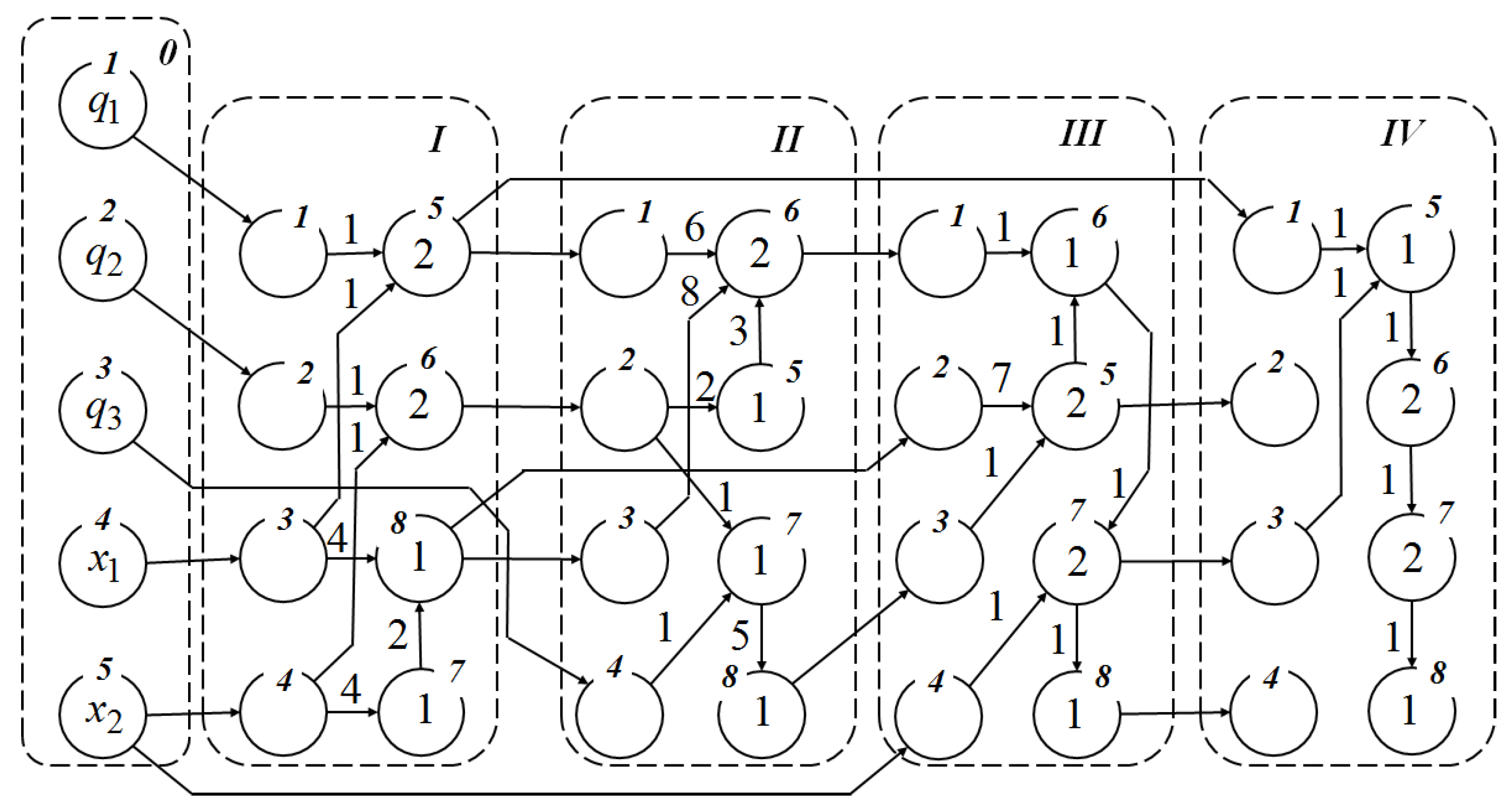
Suppose that a multilayer network operator has $K=4$ layers or subgraphs. Suppose that the number of nodes is equal to 8, and four of them are source nodes, $n_0=4$. Each layer has the same number of source nodes, some of which may not be used. The graph of a multilayer network operator for Equation (11) is shown in Figure 1.

In Figure 1, the source nodes of the graph contain the indices of binary functions; next to the edges are the indices of unary functions. To calculate a mathematical expression, it is necessary to specify the matrix of connections $D$. This matrix has dimensions of $K\times 2n_0$. Each row of the matrix is associated with a specific layer and indicates the source nodes of this layer. The odd element of the row contains the index of the layer. If the index is equal to 0 then it is a set of arguments. The even element of the row indicates the node number of this layer or the element number in the argument set. For the multilayer network operator in Figure 1, the matrix of connections has the form

$$D=\left[\begin{array}{cccccccc}0& 1& 0& 2& 0& 4& 0& 5\\ 1& 5& 1& 6& 1& 8& 0& 3\\ 2& 6& 1& 8& 2& 8& 0& 5\\ 1& 5& 3& 5& 3& 7& 3& 8\end{array}\right].$$

The network operator matrices of the four layers are

$$\begin{gathered} {\Psi }^1=\left[\begin{array}{cccccccc}0& 0& 0& 0& 1& 0& 0& 0\\ 0& 0& 0& 0& 0& 1& 0& 0\\ 0& 0& 0& 0& 1& 0& 0& 4\\ 0& 0& 0& 0& 0& 1& 4& 0\\ 0& 0& 0& 0& 2& 0& 0& 0\\ 0& 0& 0& 0& 0& 2& 0& 0\\ 0& 0& 0& 0& 0& 0& 1& 2\\ 0& 0& 0& 0& 0& 0& 0& 1\end{array}\right], {\Psi }^2=\left[\begin{array}{cccccccc}0& 0& 0& 0& 0& 6& 0& 0\\ 0& 0& 0& 0& 2& 0& 1& 0\\ 0& 0& 0& 0& 0& 8& 0& 0\\ 0& 0& 0& 0& 0& 0& 1& 0\\ 0& 0& 0& 0& 1& 3& 0& 0\\ 0& 0& 0& 0& 0& 2& 0& 0\\ 0& 0& 0& 0& 0& 0& 1& 5\\ 0& 0& 0& 0& 0& 0& 0& 1\end{array}\right], \\ {\Psi }^3=\left[\begin{array}{cccccccc}0& 0& 0& 0& 0& 6& 0& 0\\ 0& 0& 0& 0& 7& 0& 0& 0\\ 0& 0& 0& 0& 1& 0& 0& 0\\ 0& 0& 0& 0& 0& 0& 1& 0\\ 0& 0& 0& 0& 2& 1& 0& 0\\ 0& 0& 0& 0& 0& 1& 1& 0\\ 0& 0& 0& 0& 0& 0& 2& 1\\ 0& 0& 0& 0& 0& 0& 0& 1\end{array}\right], {\Psi }^4=\left[\begin{array}{cccccccc}0& 0& 0& 0& 1& 0& 0& 0\\ 0& 0& 0& 0& 0& 0& 0& 0\\ 0& 0& 0& 0& 1& 0& 0& 0\\ 0& 0& 0& 0& 0& 0& 0& 0\\ 0& 0& 0& 0& 1& 1& 0& 0\\ 0& 0& 0& 0& 0& 2& 1& 0\\ 0& 0& 0& 0& 0& 0& 2& 1\\ 0& 0& 0& 0& 0& 0& 0& 1\end{array}\right]. \end{gathered}$$

Note that, when solving the synthesis problem using the symbolic regression method, direct coding is not required. In the search process, variations of codes and calculations of mathematical expressions are performed, i.e., decoding.

5. Evolutionary Methods

Evolutionary methods form a class of modern optimization algorithms that work with a set of randomly created possible solutions and apply certain modifications of these solutions. All evolutionary methods have the following common features:

-

The search process is iterative. For each search iteration, a set of possible solutions is considered.

-

Each solution takes part in avoiding local extrema and navigating to promising areas of search space.

-

Not only the best solution but also other information about the search space is preserved over the iterations and used to form new possible solutions.

-

The evolution of solutions is based on the inheritance property, in which better solutions have a greater chance of being included in next search iteration.

The efficiency of evolutionary methods is due to the right balance between exploration and exploitation search. Exploration allows investigating the whole search space for the promising areas. This part of the search process should be applied to the search space as broadly as possible. On the other hand, exploitation involves a local search in promising areas to ensure higher accuracy of the solution. The methods of performing exploration and exploitation searches and the balance between them differ from one evolutionary method to another.

The first and the most well-known of the evolutionary methods is the genetic algorithm (GA) [20]. This method was inspired by Darwin evolution concepts. In the genetic algorithm, operators of crossover and mutation were introduced to modify a set of possible solutions in search for a best one. In this method, each possible solution is encoded with a Gray binary code and called a chromosome, whereas each search iteration is called a generation. Analogous to Darwin’s theory, better solutions have a higher probability of participating in generating new chromosomes for the next generation. However, taking into account only the best solution may lead to premature convergence to some local extremum. To prevent this, similar solutions should not be used during crossover. The mutation operator also helps not to get stuck in a local extremum. The probability of mutation, the probability of crossing depending on the quality of solutions, and their proximity are the main tuning parameters of the genetic algorithm.

Another well-known and popular evolutionary method is particle swarm optimization (PSO) [21,22,23]. As the method’s name suggests, it mimics the social behavior of some creatures in nature which exist in swarms. PSO was proposed in 1995 and gained popularity due to its effective way of combining exploration and exploitation searches during the solution modification. In this method, possible solutions are called particles. These particles are distributed in the search space and seek better positions by taking into account the best particle and the best position in previous iterations. This technique can be seen in flocks of birds or in schools of fish and is called social intelligence. The movement toward the global best solution is part of the exploitation search. The inertial movement and the movement toward the best position is part of the exploration search. The balance among these three components of the particle movement is determined by the corresponding tuning parameters of the method.

The observation of the collective behavior of bees in finding nectar sources prompted the creation of the bee algorithm (BA) [24]. In this evolutionary method, the exploration part of the search is represented by a random search of the whole search space. The analogous process among bees is the process of looking for promising places with high nectar concentration by scout bees. The found solutions can be divided into highly interesting, interesting, and not interesting. Not interesting solutions are substituted by new randomly created ones. The subdomains of given radii of highly interesting and interesting solutions are investigated more intensively. A given number of randomly created solutions are distributed within these subdomains. It is obvious that highly interesting subdomains get more attention. Best found solutions within each subdomain succeed to the next iteration. The radii of highly interesting and interesting subdomains decrease with each iteration. This ensures the success of the exploitation search. The main tuning parameters of the bee algorithm are the number of additional solutions in subdomains and their initial radii.

The gray wolf optimizer (GWO) is the most recent evolutionary method used in the study [25]. It appeared in 2014. This optimization method was inspired by the social behavior of a pack of wolves during hunting. The leader of the pack is called the alpha. The alpha always participates in the hunting process and coordinates it. Next in the wolf pack hierarchy are betas and deltas, which help in attacking prey. In a mathematical model of this hierarchy, the alpha is the current best solution, whereas the second and third best solutions are the beta and delta, respectively. For each search iteration, the three best possible solutions (alpha, beta, and delta) are selected from the set of all possible solutions. The modification of each possible solution is performed with respect to the positions of alpha, beta, and delta. The balance between exploration and exploitation search is achieved by a special component that is linearly decreased over iterations. The main advantage of the gray wolf optimizer with respect to the methods discussed above is that it is free of any tuning parameters.

When developed, all evolutionary algorithms are tested on benchmark functions that may have many local minima. An algorithm is considered satisfactory if it finds a global optimum. To increase the probability of finding the global optimum, it is necessary to enlarge parameters such as the population size and the number of generations.

6. Simulation Results

In both considered approaches, we needed to solve the finite-dimensional problem of nonlinear programming. The methods recommended in [18] for solving nonlinear programming problems require the quality criterion to satisfy the conditions of smoothness, convexity, and unimodality. In most applied optimal control problems, satisfaction of these conditions cannot be fulfilled. The application of evolutionary methods for solving nonlinear programming problems does not impose the abovementioned conditions on the quality criterion. Recent research has shown the high efficiency of evolutionary methods for solving optimal control problems [19].

To estimate the complexity of algorithms, we used the average number of objective function calculations required to obtain a result, $Y_{avg}$. Parameters of the algorithms were selected such that the number of objective function calculations $Y_{avg}$ for different algorithms was nearly the same.

The following parameters were used in computational experiments: $N=4$, $t^{+}=2.8$, $\mathsf{\epsilon }=0.01$, $x_1^1(0)=0$, $x_2^1(0)=0$, $x_3^1(0)=0$, $x_1^2(0)=0$, $x_2^2(0)=5$, $x_3^2(0)=0$, $x_1^3(0)=0$, $x_2^3(0)=10$, $x_3^3(0)=0$, $x_1^4(0)=0$, $x_2^4(0)=15$, $x_3^4(0)=0$, $x_1^{f,1}=15$, $x_2^{f,1}=10$, $x_3^{f,1}=0$, $x_1^{f,2}=15$, $x_2^{f,2}=15$, $x_3^{f,2}=0$, $x_1^{f,3}=15$, $x_2^{f,3}=0$, $x_3^{f,3}=0$, $x_1^{f,4}=15$, $x_2^{f,4}=5$, $x_3^{f,4}=0$, $x_1^{*,1}=5$, $x_2^{*,1}=5$, $x_1^{*,2}=10$, $x_2^{*,2}=10$, $r_1=r_2=3$, $r_0=2$, $u_1^{-}=-10$, $u_1^{+}=10$, $u_2^{-}=-10$, $u_2^{+}=10$, $q_{}^{-}=-20$, $q^{+}=20$, and $\Delta t=0.25$.

A detailed description of used evolutionary algorithms for both approaches was provided in [19]. For a group of four robots, we searched using a vector of 12 parameters × 2 controls × 4 robots = 96 elements.

The results of computational experiments for the optimal control problem solution using the direct approach are given in

Table 1. The results of experiments: direct approach.

No.	GA	PSO	BA	GWO	RS
1	5.48	4.52	12.74	7.71	14.77
2	5.06	4.45	9.82	11.43	17.25
3	5.29	5.38	9.58	10.71	13.8
4	6.64	5.78	11.75	8.82	18.67
5	5.54	2.81	12.95	9.4	13.56
6	7.03	6.25	13.73	9.51	16.6
7	4.43	3.27	9.97	6.55	18.02
8	3.7	3.56	11.67	10.08	19.9
9	4.43	5.9	9.67	11.23	12.81
10	7.21	3.69	13.89	9.76	12.86
$J_{avg}$	5.5	4.57	11.59	9.53	15.83
$Y_{avg}$	260.512	250.102	233.490	241.730	247.503

. Table 1 contains the mean values of objective function $J_{avg}$ and average complexity estimation $Y_{avg}$, i.e., the number of functional calculations. Note that, in Table 1, each row from 1 to 10 contains the results of one experiment for each algorithm.

Results presented in Table 1 show that all evolutionary algorithms performed better than the random search. Furthermore, PSO and GA solved the problem more effectively.

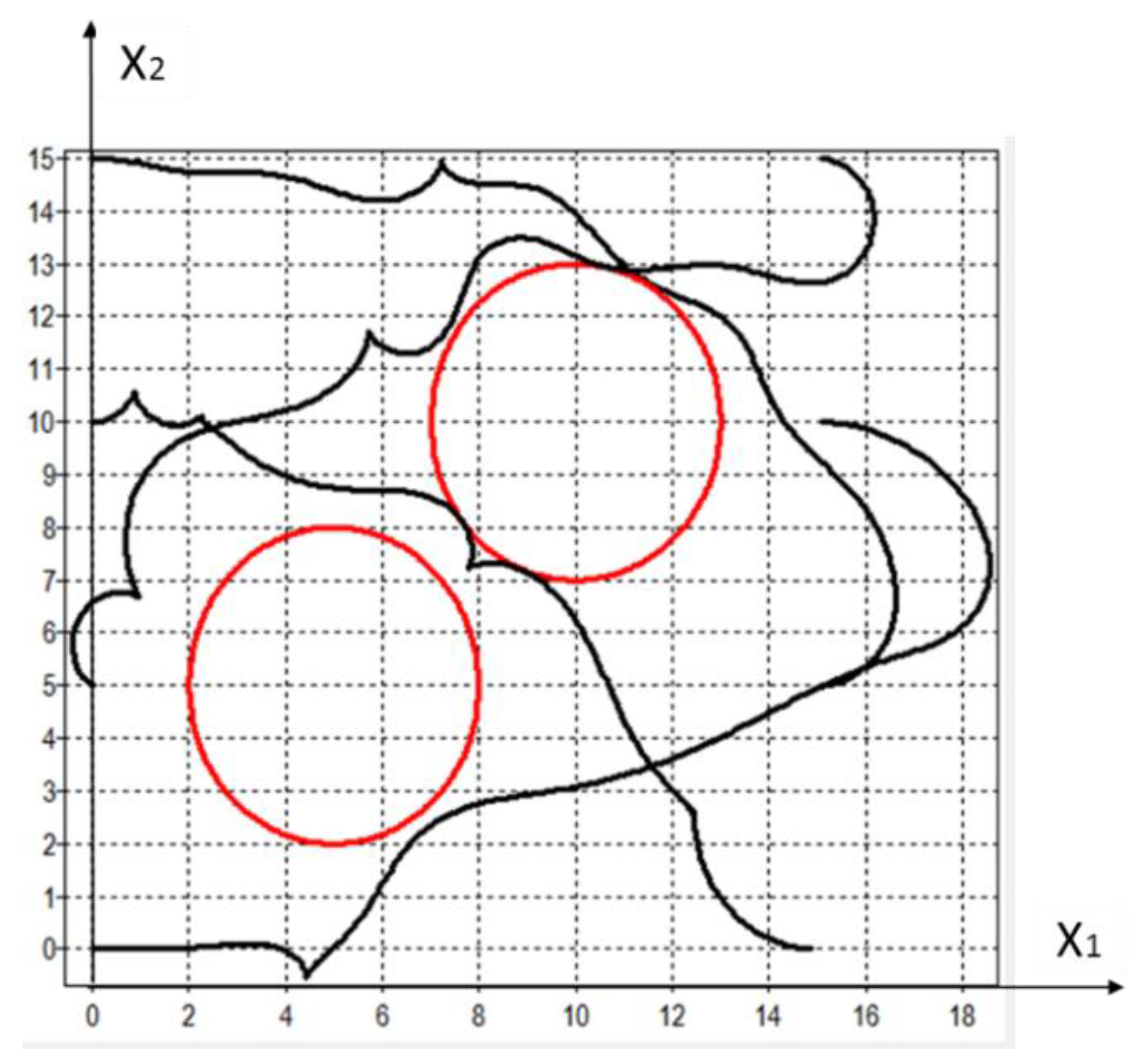
Figure 2 shows the trajectories of robots that bypassed the obstacles (circles) with control obtained using PSO, $J=2.81$. As can be seen from Figure 2, PSO found the optimal solution that ensured the attainment of terminal conditions with given accuracy without violation of the phase constraints and without collisions. The trajectories of the robots had a certain excess length.

In the second approach with synthesized control, we first solved a control synthesis problem relative to the point in the state space. Since all robots were identical, then the synthesized control function in Equation (13) was used for each robot.

Then, we solved a finite-dimensional optimization problem and searched for stabilization points ${\tilde{x}}_i^{j,k}$, where $i$ is an index of the element in the state vector, $i=\overline{1,3}$, $j$ is a robot index, $j=\overline{1,4}$, and $k$ is a point index.

The switch from one point to another was performed after each time interval $\Delta t=0.7$. For each robot, we searched three points and one known terminal point. Thus, we searched using a vector of $3·4·(\lfloor 2.8/0.7\rfloor -1)=36$ elements.

The following parameters were used in computational experiments: $u_1^{-}=-10$, $u_1^{+}=10$, $u_2^{-}=-10$, $u_2^{+}=10$, $q_{}^{-}=-20$, $q^{+}=20$, $q_1^{-}=-1$, $q_2^{-}=-1$, $q_3^{-}=-1.57$, $q_1^{+}=16$, $q_2^{+}=16$, and $q_3^{+}=1.57$. Additional parameters of the algorithms were as follows GA: H = 256, p_m = 0.7, W = 288; PSO: H = 32, W = 2048, $\mathsf{\alpha }=0.72$, $\mathsf{\beta }=0.5$, $\mathsf{\gamma }=0.1$, $\mathsf{\delta }=1$; BA: H = 30, W = 198, ${\mathsf{\alpha }}^e=0.95$, ${\mathsf{\alpha }}^s=0.95$$r^e=4$, $r^s=4$; GWO: H = 32, W = 2048, where p_m is the probability of mutation, H is the size of the population, and W is the number of generations.

The average number of objective function calculations $Y_{avg}$ was set smaller than in the direct approach because the simulation of synthesized control was very time-consuming. The results of computational experiments are given in

Table 2. The results of experiments: synthesized control.

No.	GA	PSO	BA	GWO	RS
1	2.8	2.81	2.98	2.89	7.75
2	2.69	2.86	4.24	6.29	6.86
3	2.73	2.84	3.72	2.83	8.77
4	2.86	2.63	3.13	2.83	6.2
5	2.59	2.75	3.28	2.86	10.24
6	2.74	2.86	3.72	2.87	6.7
7	2.79	2.64	3.23	2.85	8.59
8	2.93	2.62	4.22	2.49	9.74
9	2.79	2.66	3.7	2.65	5.56
10	2.67	2.87	4.17	2.88	10.29
$J_{avg}$	2.76	2.75	3.64	3.15	8.07
$Y_{avg}$	63.477	65.602	65.838	65.026	63.939

.

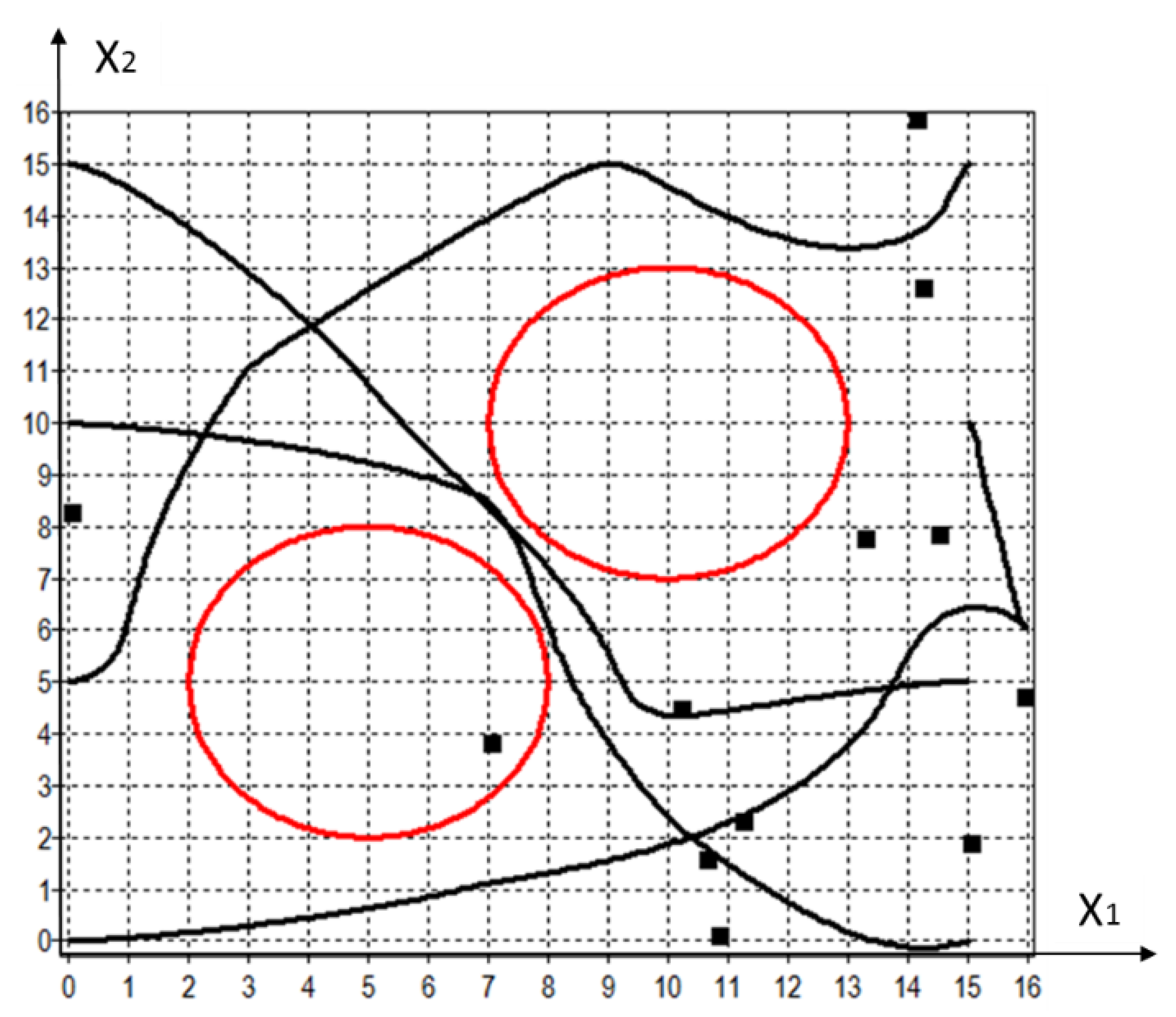
Figure 3 shows the trajectories of robots with control obtained using GWO, $J=2.49$. Here, black squares show the identified stabilization points, whereas red circles are obstacles. The paths of the robots crossed, but at different time moments; thus, they avoided collisions and did not come across obstacles. Stabilization points “attracted” the robots but did not necessarily lie on their paths. All robots reached the terminal conditions with given accuracy without violation of the phase constraints and without collisions. The trajectories of robots were smoother in comparison to those shown in Figure 2.

Despite the fact that the optimal control search using the synthesized control method required fourfold less calculation of the objective function for each method in comparison to the direct approach, the search results turned out to be much better. The best result was obtained using GWO, on average, followed by PSO.

All evolutionary techniques in both approaches performed better than the random search. We may suppose that evolutionary algorithms use certain features of intelligent search.

7. Conclusions

The optimal control problem of a group of robots with phase constraints was solved using two numerical approaches. Robots had to achieve the terminal points without collisions among themselves or with obstacles in a minimal time. The presence of phase constraints complicated the search. Evolutionary computations were applied to cope with the nonconvex and multimodal quality criterion.

In the first approach, a robotic group was treated as one object. The optimal control problem was reduced to the nonlinear programming problem. In the second approach, the problem of control synthesis was first solved separately for each robot relative to the points in the state space. To solve the synthesis problem, the multilayer network operator method was used, although this could also be achieved using other symbolic regression methods that can derive mathematical expressions.

Then, the optimal control problem was considered in the original statement, where the coordinates of the stabilization points of robots were used as control. A search was carried out for three stabilization points for each of the robots. Switching between points occurred at a specified time interval. A search of the coordinates of stability points was performed using evolutionary algorithms (genetic algorithm, particle swarm optimization, bee algorithm, and gray wolf optimizer) and a random search.

After a series of 10 tests for each algorithm, they were evaluated by the average value of functional for the best solution identified. Experiments showed that, on average, the PSO algorithm was the most effective in terms of the search of parameters in the direct method and coordinates of stabilization points in synthesized control.

With respect to the application of evolutionary algorithms to the compared approaches, a synthesized control approach was proven to perform better. In the direct approach, only GA and PSO gave satisfactory results on average, whereas, in the second approach, all the evolutionary algorithms performed well and gave, on average, approximately the same results.

Currently, there are no universal numerical methods for solving optimal control problems. It is proposed to continue the study of evolutionary algorithms and consider other new evolutionary algorithms, including hybrid ones. To use evolutionary algorithms in optimal control problems, it is necessary to include phase constraints in the functional, discretize the problem, and reduce it to a nonlinear programming problem. For this purpose, the time of the control process is divided into intervals in which the control function is approximated by polynomials depending on a finite number of parameters. Furthermore, the search for the values of the parameters of the approximating function can be carried out by evolutionary algorithms.

A distinctive feature of the application of evolutionary algorithms for solving optimal control problems is that, when calculating the value of the quality criterion, it is necessary to integrate a system of differential equations that describe the mathematical model of the control object with an approximating control function.