Prognostic Validity of Statistical Prediction Methods Used for Talent Identification in Youth Tennis Players Based on Motor Abilities

Abstract

(1) Background: The search for talented young athletes is an important element of top-class sport. While performance profiles and suitable test tasks for talent identification have already been extensively investigated, there are few studies on statistical prediction methods for talent identification. Therefore, this long-term study examined the prognostic validity of four talent prediction methods. (2) Methods: Tennis players (N = 174; n_♀ = 62 and n_♂ = 112) at the age of eight years (U9) were examined using five physical fitness tests and four motor competence tests. Based on the test results, four predictions regarding the individual future performance were made for each participant using a linear recommendation score, a logistic regression, a discriminant analysis, and a neural network. These forecasts were then compared with the athletes’ achieved performance success at least four years later (U13‒U18). (3) Results: All four prediction methods showed a medium-to-high prognostic validity with respect to their forecasts. Their values of relative improvement over chance ranged from 0.447 (logistic regression) to 0.654 (tennis recommendation score). (4) Conclusions: However, the best results are only obtained by combining the non-linear method (neural network) with one of the linear methods. Nevertheless, 18.75% of later high-performance tennis players could not be predicted using any of the methods.

1. Introduction

In professional sport, talent identification in the junior sector is of great importance [1]. After all, nations and clubs that manage to identify and train talented young athletes early on have an advantage in later sporting competition [2,3,4]. The search for future competitive athletes, therefore, begins with young athletes. In order to find suitable players, in recent years, more and more attention has been paid to tests that are designed to map the performance of children before they begin participating in a certain sport (i.e., talent detection), and when they begin training and competition (i.e., talent identification), these are believed to reflect the potential of a child for a certain sport [5]. Compared with scouting, testing has an advantage in that it can be carried out on children who have not yet achieved any success in playing. In addition, such a method can support decision-making for selection procedures in talent development programs, which are construed to help those young athletes who aim for and have the potential for elite sports.

Tennis, like other racquet sports, is considered an early-starting sport [6,7] because players require proper perceptuo-motor skills and a sound sports-specific technique on the elite level, which often must be developed at an early age [8]. Here, the great importance of early talent identification campaigns is evident. The common feature of most campaigns is that they begin at primary school age and, based on physical fitness and motor competence tests, predict future success based on a child’s performance prerequisites profile [9,10,11,12]. This early testing and desired early start in tennis ensures that, in addition to a large number of training hours—athletes complete 20‒30 h of technical training per week, even at a young age [13]—the athletes can gain competitive experience early and over a longer period of time [14]. Moreover, this offers a good opportunity for the acquisition of technical skills because there are sensitive learning phases that promote motor learning, particularly before puberty [15,16,17,18]. Perhaps, for this reason too, national sports organizations are investing more and more effort into the systematic identification of talented young players. In this professionalized, competitive environment, a “relaxed approach” is no longer sustainable [19], and talent identification is becoming the key to national elite sport performance [20,21]. In this context, statistical analysis has advantages as compared with the usual expert ratings of trainers and scientists, and they can be used to identify talented athletes and reduce the costs of talent development [22].

However, while the previous focus of scientific talent research has been very much on the prerequisite profile of later professional tennis players [23,24,25] or the improvement of prognostic test batteries [8], there have been very few studies on actual prediction calculations in sport [26]. The resulting common practice is characterized by assessing children with specific tests and comparing their performance profile with that of professional players (top down). However, performance profiles at such a young age may still differ considerably from the later performance profile in adulthood [27]. Additionally, some factors initially considered unimportant for the sport, such as balance in soccer, may be crucial for later development and success. Baker et al. [27] describe the typical procedure as a kind of “performance identification”, as compared with the required “talent identification” (future potential). For this reason, it is necessary to follow young athletes who are tested over the long term over their careers [28,29] and objectively determine the prognosis of future performance based on all test parameters (bottom up). In addition to classical linear methods [30], non-linear methods [31,32] have become established as common forecasting methods. However, these prediction methods have not yet been tested to determine their prognostic validity.

The aim of this study was, therefore, to compare the prognostic validity of common statistical prediction methods regarding the future performance success of young tennis players based on their juvenile performance profiles. Thus, based on physical fitness and motor competence tests, the performance levels of young tennis players were examined using various statistical prediction methods, and forecasts of future success were made. The prognostic validity of these common methods can be assessed on the basis of these predictions and the later tennis performance achieved by the participants, and the analytical methods can be evaluated with regard to their practical relevance (i.e., sensitivity and specificity). In this context, it is not only about how well the respective forecasts turn out to be but also about which method can most identify talented young tennis players.

2. Materials and Methods

2.1. General Study Design

For this purpose, in a long-term study, club tennis players, at the age of 8 years (U9), were tested using two anthropometric, five physical fitness, and four motor competence tests. Using a tennis-specific recommendation score composed of weighted test performances, a discriminant analysis, a binary logistic regression, and a neural network (multilayer perceptron), four separate forecasts were made for each participant as either a future ranking player in the German tennis rankings (top performer) or as a weaker club player without a ranking (low performer). The predictions were then compared with the tennis performance achieved about 5 years later (U13‒U18). For each of the four methods, the achieved sensitivity and specificity of the prognostic classification were evaluated, and the prognostic validity levels of the methods were compared based on their values of relative improvement over chance (RIOC values; [33,34]).

2.2. Participants

The participants in this study included N = 174 junior tennis players (U13‒U18), with n_♀ = 62 female and n_♂ = 112 male athletes. The mean age of the participants was 156 ± 16 months (min = 132, max = 206). All tennis players were club players who actively participated in club matches and tournaments.

2.3. Tennis Success

In terms of performance success, junior tennis players (U13‒U18) were classified into two categories: top performers (TPs) and low performers (LPs). Players who achieved enough wins and points in ranked tournaments and were therefore listed in the current national tennis ranking lists [35,36] were classified as top performers (N = 16; n_♂ = 11, n_♀ = 5). In the group of low performers, 158 tennis players with only average performance were identified. These players were unable to perform beyond local and regional successes and at no time fulfilled the necessary requirements to obtain a national ranking. Finally, this group of low performers comprised n = 57 female tennis players and n = 101 male tennis players.

2.4. Anthropometric Characteristics and Motor Abilities at U9

All junior tennis players were already tested at U9. The U9 testing included two anthropometric, five physical fitness, and four motor competence tests. The standardization of the test items is captured in protocols, which include a detailed description of the materials, set-up, assignment, demonstration, training phase, testing phase, and test scores registrations [37]. The test tasks aimed at the diagnosis of sprint, coordination, balance, flexibility, arm and upper body strength, leg power, ball throw, and endurance performance.

2.4.1. 20 m Sprint (SP)

The time for a 20 m linear running sprint was measured by means of light gates (Brower Timing Systems; Draper, USA). The starting position was 0.3 m behind the start line. Between the two potential attempts, a break of at least 2 min was allowed. The objectivity of this test is 0.86, and its reliability is 0.96 [38].

2.4.2. Sideward Jumping (SJ)

The test involves 15 s of sideward jumping within two adjacent 50 cm × 50 cm squares. The number of two-legged jumps from one square to the other without touching a boundary line was measured. Five trial jumps were allowed before the testing began. Between the two potential attempts, a break of at least 2 min was allowed. The objectivity of this test is 0.99, and its reliability is 0.89 [37].

2.4.3. Balancing Backwards (BB)

Players were asked to balance backwards on 6 cm, 4.5 cm, and 3 cm wide beams. For each beam, the number of steps backwards taken while balanced (feet fully raised) before leaving the bar was counted. The maximum number of steps per attempt was limited to eight. For each of the three beams, two attempts were made. Thus, the result was the sum of all steps taken (maximum: 48 steps). There was a short practice period before the test was carried out. The objectivity of this test is 0.99, and the reliability is 0.73 [38].

2.4.4. Standing Bend Forward (SBF)

A standing bend forward test was performed as a flexibility test. Here, the participants attempted to reach as far as possible with their fingertips beyond their feet and hold this position for at least three seconds. The distance between the fingers and ground level was recorded in cm, and a range of very low values measured from just above ground level were recorded as negative distances. Two attempts were allowed. The objectivity of this test is 0.99, and its reliability is 0.94 [37].

2.4.5. Push-Ups (PU)

The push-up test was carried out after a short trial period. Within 40 s, the number of fully completed repetitions was counted. A complete repetition was only evaluated when the upper body was laid down. Only one attempt was allowed. The objectivity of this test is 0.98, and its reliability is 0.69 [37].

2.4.6. Sit-Ups (SU)

Similar to the push-up test, the time available for the sit-up test was limited to 40 s. After a short practice phase, only one test was granted, and the number of correctly executed sit-ups was counted. The objectivity of this test is 0.92, and its reliability is 0.74 [39].

2.4.7. Standing Long Jump (SLJ)

The standing long jump was carried out without a previous practice session. The distance of the standing jump was measured in cm (measured from the heel). A break of at least 2 min was observed between two attempts. The objectivity of this test is 0.99, and its reliability is 0.89 [37].

2.4.8. Ball Throw (BT)

The ball throw was performed from a standing position with an 80 gr ball. The distance to the impact point of the ball was measured along a line orthogonal to the point of release. The result was rounded to the nearest 10 cm. After an initial trial, three scoring attempts were made, of which only the farthest test value was used for subsequent calculations. The reliability of the ball throw test has been demonstrated in a series of our own studies, and r = 0.77 (n = 1800).

2.4.9. Six min Endurance Run (ER)

A 6 min endurance run around a volleyball pitch (9 × 18 m) was carried out. There, the number of meters covered was measured. The test was conducted in groups of 15 persons at the same time. The objectivity of this test is 0.87, and the reliability is 0.92 [37].

All players were assessed under similar conditions. The tests were carried out during regular school hours (8‒12 a.m.) by qualified test personnel. The testing always began after a uniform warm-up phase with the 20 m sprint and ended with the 6 min endurance run. In all tests, except for sideward jumping (where the average of the two attempts was taken as test result), the better of the attempts counted.

Table 1. An example of test data acquisition.

Sex	Age	TP	Height	Weight	SP	SJ	BB	SBF	PU	SU	SLJ	BT	ER
1	97	1	132	27.3	4.21	33	38	4	17	23	153	19	1078
0	94	0	129	27.3	4.45	27	30	–2	14	19	135	14	959

Legend: Sex (1 = female, 0 = male); Age (months); TP = top performer (1 = yes, 0 = no); Height (cm); Weight (kg); SP = sprint (seconds); SJ = sideward jumping (repeats); BB = balancing backwards (steps); SBF = standing bend forward (cm); PU = push-ups (repeats); SU = sit-ups (repeats); SLJ = standing long jump (cm); BT = ball throw (m); ER = endurance run (m).

shows a typical dataset for two participants tested in U9 (each row represents one participant). In addition to the nine general motor test items and the anthropometric parameters, gender and test age (in months) were also recorded. Additionally, the ranking success (TP) achieved at junior age was recorded later.

All tests (with the exception of the ball throw) have been examined in a series of studies by various authors [37,38,39] with regard to the test standards. The results show high objectivity and reliability coefficients, even if these vary considerably between tests. The average total retest reliability of the eight test items (without the ball throw) is r_general = 0.85. The objectivity of the test battery is r_obj = 0.95 (range: 0.87–0.99). However, the validity of the test procedures has not yet been sufficiently verified. While Bös et al. [37] have focused primarily on content-logical validity and mainly used expert ratings (expert rating: M = 1.83; with grades from 1 to 5), other authors have used correlations to check the criterion-related validity or confirmatory factor analyses to determine construct validity [40]. For most of the individual tests, sufficient to very good test validity can be attested to for the latter two validity categories (r_validity = 0.69). Thus far, there are no major studies on prognostic validity.

2.5. Statistical Analyses

All evaluations and analyses were performed using SPSS (Version 26.0; SPSS Inc., Chicago, IL, USA), and the (bilateral) significance level was set to p < 0.05. Unless otherwise indicated, significant findings in figures and tables are marked with *. Significance values of p < 0.01 are marked with **.

Some studies [29,41,42] show that age can have a direct influence on test results. To eliminate such an age bias, a univariate analysis of variance (ANOVA) was used for all test variables to examine these data for significant differences in the U9 age groups of boys and girls. It was found that performance increases with age. In order to avoid these relative age effects, all data were first separated according to gender and then further calculated for both datasets independently. In each of the two datasets, bivariate linear regressions were then calculated for each test item separately, and the resulting residuals were saved. In these regressions, age (in months) served as the independent variable, and the respective single test served as the dependent variable. The respective residuals were finally z-standardized, and these z-standardized residual values for both gender groups were merged once again [43,44,45]. This resulted in an age-independent and gender-independent overall dataset, which was used for all further calculations. For the sake of simplicity, these z-standardized residuals are now called z-values for subsequent analyses. In addition, the prefix of the z-values for the 20 m sprint was inverted to allow for an easier comparison with the other test values. The z-values were approximately normally distributed, as shown by the Shapiro–Wilk test (p > 0.05) and a visual inspection of the histograms.

2.5.1. Prediction Methods

Because talent-detection campaigns differ in their prediction processes, four methods of recommendation calculation were analyzed and compared. In addition to a classical linear method using a tennis-specific recommendation score (weighting), a (binary) logistic regression, a linear discriminant analysis, and a neural network (multilayer perceptron) were used. All calculations were performed using the selection rate of the forecasts provided by SPSS. In each of the three classification analyses, that is, (binary) logistic regression, discriminant analysis, and neural network, junior tennis players’ performance (top performer or low performer) was used as the outcome variable (dependent variable), and the z-standardized test scores (z-values) of the U9 tests were used as input variables (independent variables). The linearly calculated tennis recommendation score was used as an external classification criterion [26].

For the three analysis methods, linear regression, discriminant analysis, and neural network (multilayer perceptron), the data were divided into five equally sized random subsets prior to the calculations. Four subsets (80% of the data) were used to create or train the respective analysis method. Using the remaining 20% (test set or hold-out), the classification method was finally tested. This calculation method was performed a total of five times, so that each of the five subsets was used once as a test set (hold-out). The test set (hold-out) results were then averaged. This procedure is known as k-fold cross-validation (CV; with k = 5). It is intended to prevent an analysis method from having already seen a case to be classified in training. The results correspond therefore rather to a situation from practice, in which usually an unknown person is to be classified. However, since the random selection of the five subsets can also have an influence on the classification results, according to Kolias et al. [46], the 5-fold cross-validation was performed five times using different random subsets, and the resulting test set classifications were averaged over all 25 predictions (5-fold 5-sample CV). To ensure a comparison of the methods, the same random partitions were used for all three methods.

2.5.2. Tennis-Specific Recommendation Score

The Tennis-Specific Recommendation Score (TRS) is based on a tennis-specific weighting of individual tests for talent identification. The TRS was established on the basis of expert ratings and derived from empirical tests of professional, adult ranked tennis players [26]. It can therefore be considered an external talent criterion. It was calculated separately for each participant and indicates the suitability of the child’s talent make-up for the particular demands of tennis. The test values of body height, body mass index (BMI), standing long jump, 20 m sprint, ball throw, sideward jumping, 6 min endurance run, balancing backward, and bend forward were included according to Formula (1).

$$\begin{array}{l}{z}_{TRS}=[2.0\times z_{standing long jump}+1.8\times z_{sideward jumping}+1.7\times z_{height}\\ +1.3\times \left(z_{sprint}+z_{balancing}-z_{bmi}\right)\\ +1.2\times \left(z_{ball throw}+z_{bend forward}\right)+1.1\times z_{endurance run}]\\ ÷12.9\end{array}$$

(1)

Due to the specific calculation involved, z_TRS is comparable to a normal z-value. Thus, also here, a value of z_TRS = 0 indicates average suitability. In order not only to give a general tennis recommendation (z_TRS > 0) but also to predict future top performers, it is necessary to define a suitable threshold value, above which a participant is assigned to the group of potential top performers. Sensitivity and specificity can thus be determined using the selected threshold value, e.g., z_TRS = 1.3. In this example, the chosen z-value of z_TRS = 1.3 corresponds to a selection rate of 10%, which is close to the observed percentage of top performers in this sample (16/174 = 10.875%). Thus, using this method, participants with z_TRS ≥ 1.3 were automatically predicted to be top performers, and participants with z_TRS < 1.3 were predicted to be low performers.

2.5.3. Binary Logistic Regression Analysis

A binary logistic regression examines the influence of independent variables on a binary-coded dependent variable. Thus, the influence of the test values on later tennis performance was determined in this way. The group of youth top performers was marked with a “1”, and the group of low performers was marked with a “0”. Because the “Enter” method was chosen, all variables of a block were recorded in common in one step, and their influence on the regression was evaluated simultaneously. In trial calculations, it was found that the results of the “backward” and “forward” method in the classification correspond to those of the “Enter” method. Based on the multiple regression, the output is also presented as a categorical variable, and therefore, it is possible to predict affiliation with a performance group. Sensitivity and specificity can be easily calculated. The separation value of this categorical output variable was u_cut = 0.5 by default for these analyses. This means that, with an individual output value of u_cut ≥ 0.5, the participant was recommended as a top performer. In order to represent a valid and also practical result, the logistic regression was performed as a k-fold cross-validation (k = 5), and this procedure was repeated five times. The results of the 25 individual analyses were ultimately averaged.

2.5.4. Discriminant Analysis

Discriminant analysis can be used to investigate differences in feature profiles of different groups and then to assign an unknown profile to a suitable group. Similar to binary logistic regression, group memberships are calculated, and thus the sensitivity and specificity can be analyzed. Since the grouping variable “tennis performance” had only two values (top performer/low performer), only one discriminant function was determined. Using the discriminant coefficients of this function, a performance prediction could be calculated for each single hold-out case. Since the group variable was dichotomous, the recommendation calculation was performed using a linear method similar to binary logistic regression. The a priori probability of the groups was assumed to be 50:50 (settings: groups equal). For a practical investigation, a 5-fold cross-validated procedure was also considered This procedure was repeated five times with different partition groups, and the results were averaged (see Binary Logistic Regression Analysis and Neural Network Analysis). The individual talent characteristics profile (hold-out) of the required athlete was therefore not already in the training group, making the identification of the case more difficult. This form of analysis therefore offers lesser sensitivity and specificity but corresponds more closely to the “natural” application of talent prognosis in sports practice.

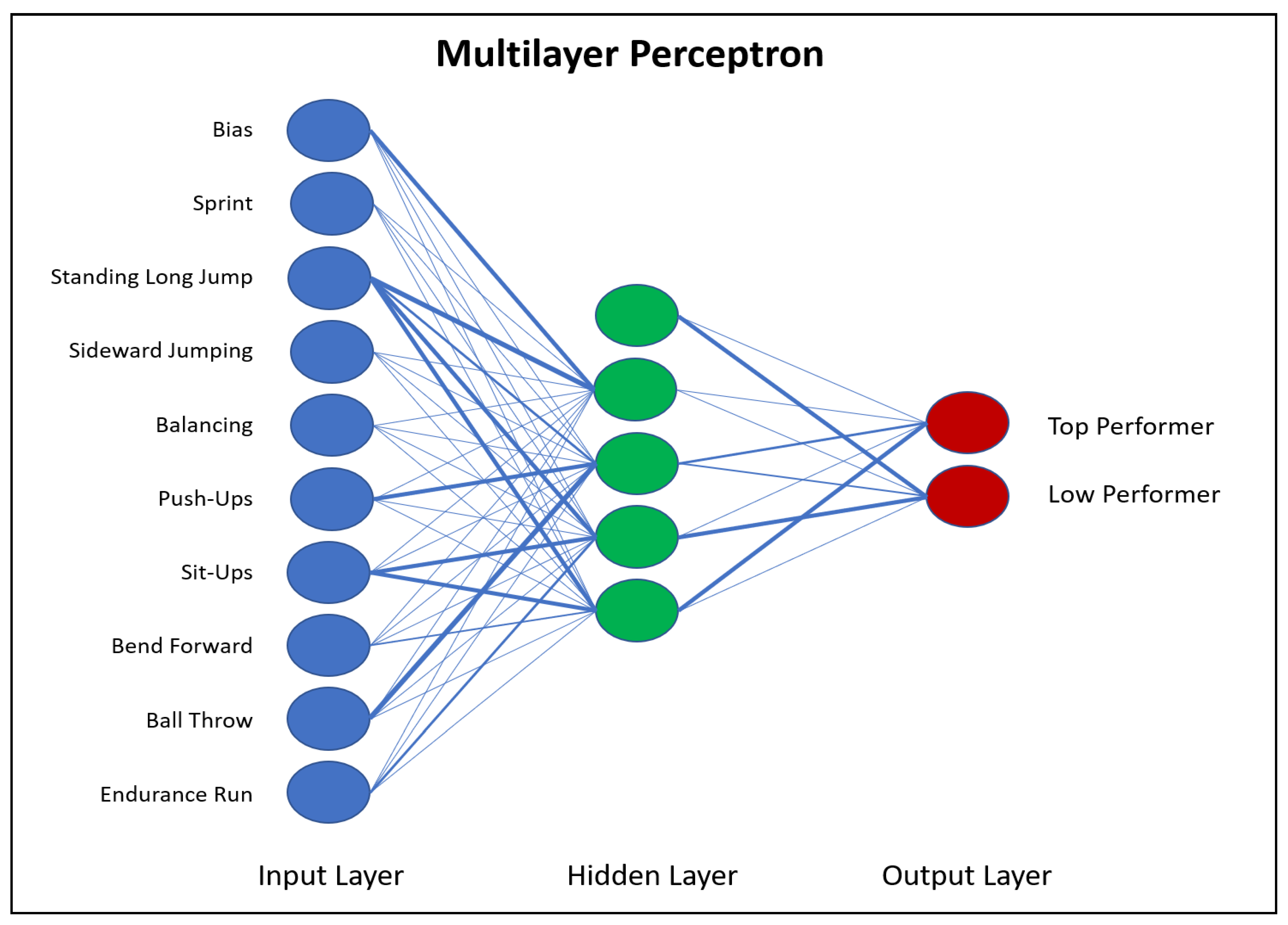
2.5.5. Neural Network Analysis

In contrast to the three more traditional linear or multilinear prediction methods, a neural network (multilayer perceptron) was applied as the fourth type of analysis. Thus, with the multilayer perceptron (MLP) tool from SPSS 26 (IBM), a non-linear “feed-forward” classification procedure was used to analyze the prognostic validity of the group assignment [47,48].

The classification calculation of the neural network (SPSS 26) is composed of three basic parts training, validation, and test (hold-out). The network weights are mainly determined via training, with validation measuring the model errors. Only the test set is independent of the creation of the network, which provides an honest estimate of the predictive power of the model. The distribution of the training, validation, and test (hold-out) components was carried out for smaller groups, as in the present case, according to a 60-20-20 scheme [49,50]. Each part (training, validation, and test) is randomly selected from the total sample. The calculations for the neural network therefore corresponded to the 5-fold CV already used in the logistic regression and discriminant analysis. Again, the 5-fold CV was repeated using five different partition divisions [46] and the corresponding 25 test classifications were averaged (5-fold 5-sample CV). Additionally, this method is intended to compensate for the small dataset and avoid misinterpretation due to volatile parameter estimates [51].

The architecture of the network contained the eleven test variables (z-values) as input neurons (covariates without additional scaling or normalization) and the two performance classes (top performer/low performer) as output neurons (dependent variable). The neurons of one hidden layer in-between were generated by the program independently and depended on a randomly chosen training start vector. Due to the small amount of data, the architecture was limited to a maximum of one hidden layer with one to ten neurons [45]. However, in various test calculations with the data set used here, it was shown that even with different start vectors, the calculated neural network solutions never exceeded more than five neurons (plus one bias neuron) in the hidden layer. Figure 1 shows a typical example of the (fully connected) neural network with nine input neurons (+1 bias neuron), four neurons (+1 bias neuron) in the hidden layer, and the two output neurons of the binary target variable (Figure 1). Experimental calculations with several hidden layers showed no significant improvements in the network. The learning of the network is iteration-based and terminated when no further reduction of the error quotient is apparent. The type of training used was “batch training” [52], which is the recommended method for smaller datasets. All other settings were selected according to the default settings of SPSS.

2.5.6. Prognostic Validity of the Analyses

Prognostic validity can be determined by the theoretical accuracy (sensitivity and specificity) of the performance forecasts of the various prediction methods. For all calculations of the parameters of the analysis methods, only the classification results of the corresponding hold-outs were used.

Table 2. Example for sensitivity and specificity calculation.

		Predicted/Recommended
		Low Performer	Top Performer	∑
Observed/Existing	Top Performer	C	A	A + C
	Low Performer	D	B	B + D
	∑	C + D	A + B	A + B + C + D

represents a typical example of a 2 × 2 classification table. Variable A corresponds to true-positive predictions, B to false-positive predictions, C to false-negative predictions, and D to true-negative predictions.

Sensitivity (recall; Formula (2)) indicates how many top performers (A = true positives) from the observed group (A + C = 16) were correctly predicted. For example, if twelve top performers were correctly identified/classified as top performers, the sensitivity is 75%. The specificity (Formula (3)) represents the percentage of correctly predicted low performers (D = true negatives) in the group of low performers (B + D).

$$\mathrm{Sensitivity}=\frac{\mathrm{A}}{\mathrm{A}+\mathrm{C}}$$

(2)

$$\mathrm{Specificity}=\frac{\mathrm{D}}{\mathrm{B}+\mathrm{D}}$$

(3)

Furthermore, the positive and negative predictive values (Formulas 4 and 5) of the predictions were determined (positive predictive value = precision). These two parameters indicate the probability of actually living out a corresponding forecast. It therefore corresponds to the percentage of predictions that actually occurred.

$$\mathrm{Positive}\mathrm{Predictive}\mathrm{Value}=\frac{\mathrm{A}}{\mathrm{A}+\mathrm{B}}$$

(4)

$$\mathrm{Negativ}\mathrm{Predictive}\mathrm{Value}=\frac{\mathrm{D}}{\mathrm{C}+\mathrm{D}}$$

(5)

In general, the hit rate is the percentage of correctly predicted recommendations. Accordingly, the true-positive predictions (A) and the true-negative predictions (B) are added together and divided by the total sample size (Formula (6)). To calculate the random hit rate (Formula (8)), the selection rate (S) is needed. The selection rate is the percentage of top performer recommendations among all recommendations (Formula (7)). It is determined in advance or via the analysis types. Using the selection rate, the random hit rate (Formula (8)) can now be determined. For this purpose, the selection rate (S) is multiplied by the number of existing top performers (A + C). This calculates the number of correct top performer recommendations in a random draw from the group of top performers. In addition, the number of correct low performer recommendations in a random draw from the group of low performers (B + D) is also determined. This is done using the counter-probability of the selection probability (1 − S). Both values are then summed and divided by the total sample size to obtain the random hit rate. The maximum hit rate can also be easily calculated using the counter-probability (Formula (9)). To do so, the over-recommendation of a group caused by the selection rate is subtracted from the total probability (=1). For example, if 20 top-performer recommendations (A + B) have been made by an analysis (selection rate = 11.5%) and only 16 top performers (A + C) exist (~9.2%), then four recommendations ([A + B] − [A + C]) are automatically wrong (~2.3%). Therefore, these false over-recommendations are eliminated, and the maximum hit rate would be 97.7%. The number of over-recommended cases is obtained by subtracting false-positive (B) cases from false-negative (C) cases ([A + B] ‒ [A + C] = B − C). If there is an under-recommendation and fewer than 16 top performer recommendations are made, the subtraction is reversed (C − B). Both can be expressed in a simplified way via |B − C| (see Formula (9)).

$$\mathrm{Hit}\mathrm{Rate}=\frac{\mathrm{A}+\mathrm{D}}{\mathrm{A}+\mathrm{B}+\mathrm{C}+\mathrm{D}}$$

(6)

$$\mathrm{Selection}\mathrm{Rate}=\mathrm{S}=\frac{\mathrm{A}+\mathrm{B}}{\mathrm{A}+\mathrm{B}+\mathrm{C}+\mathrm{D}}$$

(7)

$$\mathrm{Random}\mathrm{Hit}\mathrm{Rate}=\frac{\mathrm{S}\times \left(\mathrm{A}+\mathrm{C}\right)+\left(1-\mathrm{S}\right)\times \left(\mathrm{B}+\mathrm{D}\right)}{\mathrm{A}+\mathrm{B}+\mathrm{C}+\mathrm{D}}$$

(8)

$$\mathrm{Maximum}\mathrm{Hit}\mathrm{Rate}=1-\frac{\left|\mathrm{B}-\mathrm{C}\right|}{\mathrm{A}+\mathrm{B}+\mathrm{C}+\mathrm{D}}$$

(9)

Because the numbers of top performer forecasts (selection rate) can vary between methods, an RIOC value (Relative Improvement Over Chance; [33,34]) was ultimately calculated for each method (x_RIOC). This value determines the relative hit accuracy. In most analyses, a maximum hit rate of 100% cannot be achieved. This can lead to a misinterpretation of the validity parameters (e.g., phi or kappa; [34]). The RIOC index avoids this problem by calculating the actual hit rate in relation to the potential maximum hit rate (see Formula (10)).

$$x_{RIOC}=\frac{\mathrm{hit}\mathrm{rate}-\mathrm{random}\mathrm{hit}\mathrm{rate}}{\max .\mathrm{hit}\mathrm{rate}-\mathrm{random}\mathrm{hit}\mathrm{rate}}$$

(10)

The calculated value varies, usually in the range 0 < x_RIOC ≤ 1, but it can also have negative values. With a value of x_RIOC = 0.33, the classification is considered good. Above 0.66 is considered very good [53]. Using this calculation scheme, the four methods can be directly compared and evaluated independent of their actual selection rates. The real selection rate for talent diagnostics and, thus, also the maximum hit rate, always depends on the talent campaigns and support programs of the participating countries, and therefore, this selection rate can vary considerably in practice.

The Youden Index J (also Youden’s J) was determined as a further comparative value (Formula (11)). It is calculated by summing sensitivity and specificity, and therefore, it shows prognostic validity independent of the sizes of the two performance groups [54]. Usually, J reaches values between 0 (random result) and 1 (optimum result).

$$\mathrm{J}=\mathrm{Sensitivity}+\mathrm{Specificity}-1$$

(11)

In addition to Youden’s J, the Area Under ROC Curve [55] and F₁ score were also ways to evaluate the predictive power of an analytical method (Formula (12)). The F₁ score is based on the harmonic mean, and its calculation is equally divided between sensitivity (recall) and positive predictive value (precision). It can take values between 0 and 1, where 1 stands for the maximum predictive strength. In contrast to Youden’s J, which includes sensitivity and specificity in equal measure, the focus here is on the predictive power of true-positive cases.

$${\mathrm{F}}_1=2\times \frac{\mathrm{Sensitivity}\times \mathrm{Positive}\mathrm{Predictive}\mathrm{Value}}{\mathrm{Sensitivity}+\mathrm{Positive}\mathrm{Predictive}\mathrm{Value}}$$

(12)

2.5.7. Classification of Individual Tennis Players

In order to gain a more precise insight into the calculated prognosis, the participants predicted to be future top performers were also recorded for each type of analysis. Thus, we could determine which individual top performers were correctly identified via which method and which low performers were erroneously judged to be top performers. Using a classification map, it was therefore easy to determine how the predictions of the various analysis methods were distributed. In addition, the probability that an athlete would later become a top performer, as calculated via the various methods, was recorded.

3. Results

3.1. Test Performance

In considering the test results of the five physical fitness, four motor competence, and two anthropometric test items (U9), significant differences between later top performers and low performers (U13‒U18) can be observed. The mean values of the later top tennis players were significantly higher than those of the later low performers for nearly all test variables. While no differences could be found for body weight (p = 0.94) and bend forward (p = 0.16), all other test items showed significant differences (p ≤ 0.05). The mean values of the test items sideward jumping, balancing backwards, standing long jump, 6 min endurance run, and ball throw showed highly significant differences (p ≤ 0.01). The minimum of the sideward jumping test was MIN = 27.0 repetitions (rps) for top performers, which was only slightly below the average value of M = 27.3 rps for low performers. Additionally, for the balancing backwards, standing long jump, sit-ups, and 6 min run tests, 84% of the top performers were better than the average low performer. A maximum of 16% of low performers managed to reach the average of the top performers on the standing long jump and ball throw. All descriptive statistics for the test items can be found in

Table 3. Descriptive statistics for the two anthropometric, five physical fitness, and four motor competence diagnostics of the U9 participants.

Variables	Groups	N	M	SD	SE	95% CL		Min	Max
						LL	UL
Calendar age * (month) (Time of testing; U9)	LP	158	93.8	5.0	0.39	93.0	94.6	83	110
	TP	16	97.5	6.4	1.60	94.1	100.9	88	112
Test results
Body height * (cm)	LP	158	129.1	5.7	0.45	128.2	130.0	117	145
	TP	16	132.3	4.5	1.13	129.8	134.7	127	143
Body weight (kg)	LP	158	27.2	4.1	0.33	26.6	27.9	20.0	39.3
	TP	16	27.3	1.9	0.48	26.3	28.3	23.4	30.6
Sideward jumping ** (repeats)	LP	157	27.3	6.1	0.49	26.3	28.2	6.5	40.5
	TP	16	33.0	5.1	1.27	30.3	35.7	27.0	45.0
Balance backward ** (steps)	LP	158	30.3	8.5	0.67	28.9	31.6	8	48
	TP	16	38.3	5.7	1.42	35.2	41.3	28	48
Standing long jump ** (cm)	LP	157	135.1	16.2	1.30	132.5	137.6	82	190
	TP	16	153.0	17.2	4.30	143.8	162.2	125	178
20 m sprint * (s)	LP	158	4.45	0.36	0.03	4.39	4.51	3.10	5.32
	TP	16	4.21	0.34	0.08	4.03	4.39	3.50	4.72
Push-ups * (repeats)	LP	158	14.6	3.6	0.28	14.0	15.1	4	24
	TP	16	17.1	5.2	1.30	14.3	19.9	9	25
Sit-ups * (repeats)	LP	158	19.2	5.1	0.40	18.4	20.0	2	30
	TP	16	23.4	4.1	1.02	21.3	25.6	15	29
Bend forward (cm)	LP	158	1.98	5.94	0.47	1.05	2.92	−11	18
	TP	16	4.16	4.90	1.22	1.55	6.77	−10	12
6 min run ** (m)	LP	154	959	130.8	10.5	938	979	545	1259
	TP	16	1078	80.7	20.2	1035	1121	891	1200
Ball throw ** (m)	LP	155	13.5	4.03	0.32	12.9	14.2	3.8	27.6
	TP	16	18.8	5.35	1.34	15.9	21.6	9.2	28.3

M = mean; SD = standard deviation; SE = standard error; CL = confidence limit; LL = lower limit; UL = upper limit; Min = minimum; Max = maximum; LP = low performer; TP = top performer; * p ≤ 0.05; ** p ≤ 0.01.

.

3.2. Test Quality Parameters of the Prediction Methods

3.2.1. Tennis Recommendation Score

Using the TRS (see

Table 4. Sensitivity and specificity of the tennis recommendation score at z_TRS = 1.3.

Tennis Recommendation Score (zTRS = 1.3)		Predicted/Recommended
		Low Performer	Top Performer	Percentage Correct
	Top Performer	4	12	75%
Observed/Existing	Low Performer	131	27	82.9%
	Percentage (total)	77.6%	22.4%	82.2%

), a total of 39 of the 174 test participants (22.4%) were predicted to become talented tennis athletes (selection rate). Overall, 135 participants (77.6%) did not receive a top-level assignment because it was assumed that they could not reach the top level due to their low individual recommendation values. With a selected threshold value of z_TRS = 1.3, 12 of the 16 later top performers (75%) were true-positives (sensitivity). One hundred and thirty-one participants (82.9%) who did not reach the top level were also correctly classified as low performers, that is, true negatives (specificity). In total, 143 of 174 (82.2%) children could be correctly identified as later top or low performers via this linear method. If the talent forecasts with the same prediction rate (22.4%) were expressed at random, only 4, as compared with 12, of the top performers and 122, as compared with 131, of the low performers would be correctly predicted, and the overall prediction quality would only be 72.4%, as compared with the value of 82.2% described above. If the percentage values for sensitivity and specificity were considered in combination, the benefit is more obvious. With a cutoff limit value of z_TRS = 1.3, the Youden Index amounts to a total of 157.9% (75% + 82.9%), thus representing a 57.9% improvement as compared with a random drawing. The Area Under ROC Curve was 0.852 (standard error = 0.048; 95% confidence interval: min = 0.759, max = 0.946).

3.2.2. Logistic Regression

In addition to the TRS, a (binary) logistic regression also offers a chance to create a talent prognosis for the test participants. The 5-fold cross-validation was performed five times, and the results were averaged. The omnibus test of the model’s averaged coefficients showed a significant result (chi-square(11) = 33.67, p < 0.001). The model quality was determined based on Nagelkerke’s R-square, which had a value of 0.476. The Area Under ROC Curve was 0.810 (standard error = 0.054; 95% confidence interval: min = 0.705, max = 0.915). Overall, however, in most analyses, none of the regression coefficients showed a significant result, so this form of analysis should be interpreted with caution.

Approximately 6 of the 16 athletes who were ultimately competitively ranked were correctly identified by their test values (

Table 5. Sensitivity and specificity of the (binary) logistic regression analysis.

(Binary) Logistic Regression 1		Predicted/Recommended
		Low Performer	Top Performer	Percentage Correct
	Top Performer	10	6	37.5%
Observed/Existing	Low Performer 2	144	6	96%
	Percentage (total)	92.8%	7.2%	90.4%

¹ A 5-fold cross-validation was performed a total of five times, and the results were averaged. For a better evaluation of the results, the average values were multiplied by five. ² Eight children could not perform at least one test, so they were excluded from this analysis.

). The sensitivity was therefore 37.5%. It should be noted, however, that only about twelve children in total received a top-level prognosis in this form of analysis. The specificity was 96%. With the exception of six participants, all low performers could be correctly classified. The overall accuracy of the analysis method was 90.4%. The summed percentage result for the sensitivity and specificity of the logistic regression was 133.5%, which is 33.5% better than that of a random sample. If a random prediction were considered with the same selection rate, the sensitivity would be 7.2%. Thus, it would be 26.3% less than the sensitivity value of 33.5% achieved via the logistic regression analysis. The same applies to a random specificity. This would amount to 92.6%, as compared with the 96% achieved here, and the overall result in terms of correctly identified test participants would only be 84.4%. Among participants predicted to be future top performers via the logistic regression, 50% of such prognoses were correct (positive predictive value). This means that every second child classified as a top performer actually made it into the top group.

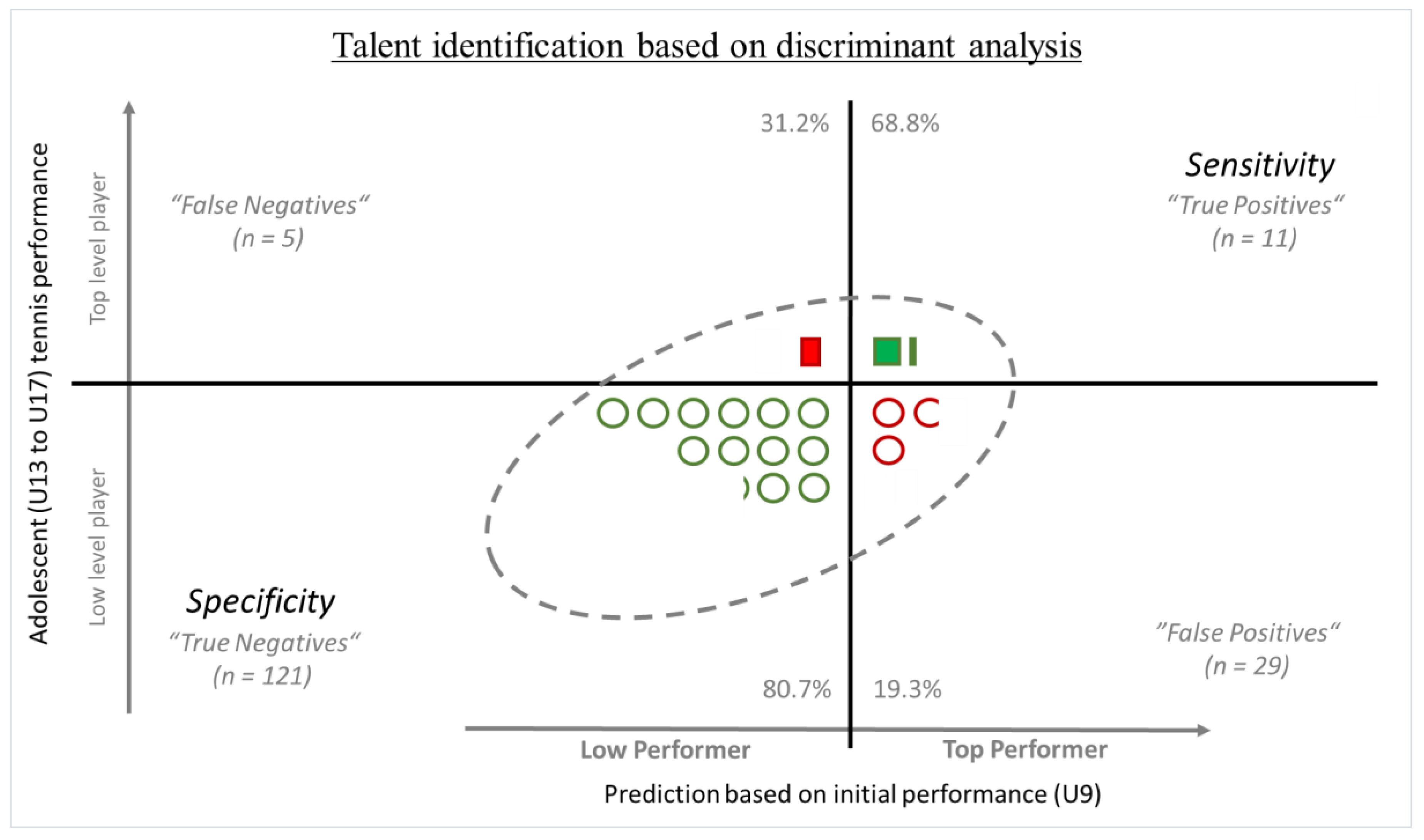
3.2.3. Discriminant Analysis

A 5-fold cross-validated discriminant analysis was calculated and repeated five times with various partitions. The corresponding results were averaged and provided another way to make talent predictions. Because there were only two service groups (binary), only one discriminant function was required here. The ability to separate the two groups can be seen in the averaged eigenvalue (this was EV = 0.286, canonical correlation: r = 0.471). Thus, the groups could be separated satisfactorily based on their group centroids. In addition, the discriminant function should now show the best possible separation. In this analysis, Wilk’s lambda was 0.775 (chi-square(11) = 31.81, p < 0.01). The Area Under ROC Curve was 0.800 (standard error = 0.069; 95% confidence interval: min = 0.663, max = 0.936). Consequently, significant differences between the two groups could be detected via the discriminant function, but the model had only a limited selectivity due to the high Wilks lambda. Nevertheless, the cross-validation classification showed good results (Figure 2).

Using this method, 11 of the 16 later top performers could be correctly identified (Figure 2). This corresponds to a sensitivity of 68.8%. Additionally, 121 of the later 150 low performers could be correctly classified (specificity of 80.7%). The overall prediction quality was thus 79.5% (132/166), and the sum of the two parameters was 149.5%. A random prediction with the same classification rate (24.1%) would result in a sensitivity of 24.1% and a specificity of 75.9%, with an overall prognostic quality of 70.9%. While the discriminant analysis differed only slightly from the random sample in specificity and total result, in sensitivity it showed a clear advantage, with 40% more true-positive hits. This means that, as compared with a random prediction, seven additional top performers could be identified via the discriminant analysis.

3.2.4. Neural Network Analysis

On average, the MLP achieved a sensitivity of 75% and a specificity of 84% (

Table 6. Sensitivity and specificity of the Neural Network (Multilayer Perceptron).

Multilayer Perceptron 1		Predicted/Recommended
		Low Performer	Top Performer	Percentage Correct
	Top Performer	4	12	75%
Observed/Existing	Low Performer 2	126	24	84%
	Percentage (total)	78.3%	21.7%	91%

¹ A 5-fold cross-validation was performed a total of five times, and the respective test results were averaged. ² Eight children could not perform at least one test, so they were excluded from this analysis.

). It could thus correctly identify approximately 12 of the 16 top performers and 126 of the 150 low performers. Taken together, these two parameters add up to 159%. The overall prognostic quality was thus 91%. If a test participant received a judgement as a later top performer, 33% of the predictions were correct. This means that, out of nine high-potential test participants, three were expected to reach the top level. Among the predicted low performers, only 3.1% of the predicted performance outcomes failed to apply. Thus, 3 out of 100 test participants reached the top level despite a negative individual forecast. Comparing the results with a random draw, the benefits of the MLP become apparent. The random sensitivity and specificity were 21.7% and 78.3%, and thus, the overall classification quality was 72.9%. Both the sensitivity and the specificity of the MLP clearly exceeded these random predictions. The Area Under ROC Curve was 0.831 (standard error = 0.056; 95% confidence interval: min = 0.721, max = 0.941).

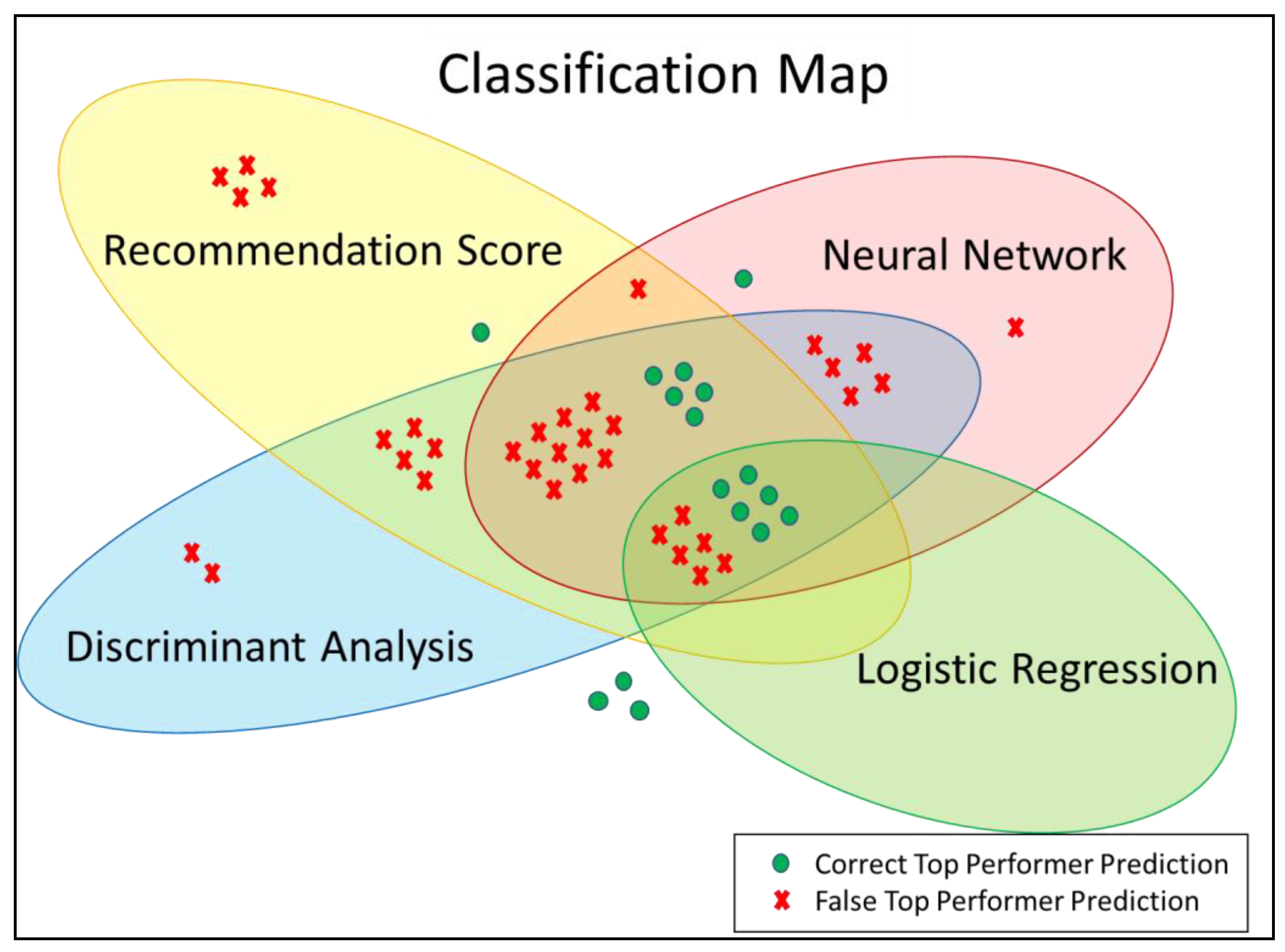
3.3. Prognostic Validity of the Prediction Methods

In the linear discriminant analysis (see Figure 2; N = 166; eight children could not perform at least one test, so they were excluded from this analysis), the sensitivity could assume values of 24.1% (random result) to 100%, with a constant selection rate of 24.1%. The specificity reached values ranging from 75.9% (random result) to 84%. Thus, accordingly to Formula (8), the random (total) hit rate was 70.9% (see Formula (13)).

$$\mathrm{Random}\mathrm{Hit}\mathrm{Rate}=\frac{0.241\times 16+\left(1-0.241\right)\times 150}{166}\approx 0.709$$

(13)

Following Formula (9), the maximum hit rate was 0.855 (Formula (14)):

$$\mathrm{Maximum}\mathrm{Hit}\mathrm{Rate}=1-\frac{\left|29-5\right|}{166}\approx 0.855$$

(14)

For this calculation, therefore, the counter-probability is used to consider what the actual probability is if only the over-recommendations lead to an incorrect prediction. With 40 top performer predictions, 24 over-recommendations occurred, which corresponds to 14.5%—accordingly, this percentage is deducted from 100%. Finally, accordingly to Formula (11), it remains to calculate the RIOC value (Formula (15)):

$$\mathrm{RIOC}\mathrm{Value}=\frac{0.795-0.709}{0.855-0.709}\approx 0.588$$

(15)

The calculations of the predictors of the other analysis methods are done analogously. All four methods revealed RIOC values in the range of 0.33–0.67 and thus illustrate a good classification result. However, the differences in the results of at least three out of four analyses were small.

The results for sensitivity and specificity are very different (

Table 7. Comparison of the prognostic validity of the four analyses.

	Recommendation Score	(Binary) Logistic Regression	Linear Discriminant Analysis	Multilayer Perceptron
Sensitivity	0.750	0.375	0.688	0.750
Specificity	0.829	0.960	0.807	0.840
Selection Rate	0.224	0.072	0.241	0.217
Positive Predictive Value	0.308	0.500	0.275	0.333
Negative Predictive Value	0.970	0.935	0.960	0.969
Random Hit Rate	0.725	0.845	0.709	0.729
Hit Rate	0.822	0.904	0.795	0.831
Maximum Hit Rat	0.868	0.976	0.855	0.880
Youden’s J	0.579	0.320	0.495	0.590
F1 score	0.437	0.429	0.393	0.462
RIOC Value	0.678	0.447	0.588	0.681

). The logistic regression shows a sensitivity of only 37.5% but reaches the highest specificity, with 96%. The TRS and MLP prediction methods reach 75% or more in both parameters. Considering the positive predictive values, more than every second prediction of a top performer is correct for the logistic regression (50%). The top performer predictions for the TRS and MLP analysis methods only apply to every third (TRS = 30.8% and MLP = 33.3%). However, their negative predictive values are higher than those of the other two methods. Youden’s J turns out to be the highest, with J = 0.59 for the MLP. This is closely followed by the TRS, with J = 0.579. Logistic regression performs worst among the four methods. Despite its high Youden’s J, the TRS only achieves a value of F₁ = 0.437 in terms of the F₁ score, which is probably related to its low positive predictive value (30.8%). Among the four methods, the MLP performs best here, with F₁ = 0.462. This is not surprising because it has the highest sensitivity and also a high positive predictive value (33.3%). The RIOC values show values above 44% for all methods, with the MLP reaching the highest value of 68.1%. If, for example, a method would correctly predict the performance of another person, the RIOC value can increase between 1% and 8% depending on the performance group and method. Thus, another correct top performer prediction would increase the RIOC value of discriminant analysis from 58.8% to almost 67%.

Combining the predictions (union set) of the TRS with those of the MLP yields the highest sensitivity of all analyses (81.3%). Of 16 top performers, 13 are recognized as such. The selection rate is 27.7%. However, with a value of 78%, the specificity is below the values of the individual analysis methods. The lower specificity also causes the overall hit rate to drop to only 78.3%. The positive predictive value is 28.3%, and the negative predictive value is 97.5%. However, in comparison with the four individual forms of analysis, this combination of methods performs above average in Youden’s J (0.593) and also in RIOC (0.741). Only the F₁ score is very low at 42%, which is due to the low positive predictive value. Looking at the intersection of the predictions of the three classification methods, TRS, MLP, and DA (see also Figure 3), the sensitivity reaches a value of 68.8% and the specificity a value of 88.7%. Due to the higher positive predictive value (0.393), the F₁ score (0.5) is the highest among all analysis methods and combinations. Youden’s J reaches a value of 57.5%, and the RIOC value is 62.4%. A combination of the other analysis methods showed no significant improvements of the results.

3.4. Classification of Individual Tennis Players

Through the various prognostic procedures, 13 out of the total of 16 later top performers were correctly identified, whereas 3 athletes could not be detected correctly by any of the methods (Figure 3). The highest number of correct assignments was produced by the artificial neural network and the TRS. With both instruments, twelve of the later top performers were correctly predicted. However, the TRS also led to the highest number of incorrect classifications (n = 27). Its positive predictive value is correspondingly low (30.8%). The artificial neural network, on the other hand, produced 24 incorrect predictions. Its positive predictive value was 33.3%. Moreover, both methods could correctly predict at least one player who could not be predicted by the other analyses. By combining the two types of analyses, 13 top performers could be classified correctly as true positives.

Six top performers and six low performers were included in the talent prognosis by all four methods. Five other top performers were additionally recognized by all methods except logistic regression. Logistic regression predicted the smallest number of top performers overall, and only those who were also recognized by other methods. However, with only twelve predictions, it has the lowest selection rate, but at the same time, with six out of twelve, it has a high rate of hits in terms of its correct identification of top performers. A combination of the methods could also provide a high positive predictive value. If only those test participants who were jointly identified in the tennis recommendation score, discriminant analysis, and neural network were judged as top performers, 11 future top performers would be correctly classified out of only 28 predictions in total (39.2%).

The probabilities at which the analysis methods made correct top-performer recommendation are plotted in

Table 8. Probability outputs of the analysis methods.

	Probability of Being a Top Performer (%)
	Recommendation Score	Logistic Regression	Discriminant Analysis	Multilayer Perceptron
Top Performer 1	99	90	99	99
Top Performer 2	97	86	98	97
Top Performer 3	93	68	97	96
Top Performer 4	96	71	96	90
Top Performer 5	83	64	95	90
Top Performer 6	89	68	90	95
Top Performer 7	91	15	68	71
Top Performer 8	79	33	85	88
Top Performer 9	55	7	65	70
Top Performer 10	66	18	63	68
Top Performer 11	57	9	58	68
Top Performer 12	67	16	41	32
Top Performer 13	44	3	23	52
Top Performer 14	40	5	24	37
Top Performer 15	20	2	9	29
Top Performer 16	33	1	1	15

Legend: The averaged test values of the cross-validation test sets (hold-out) were converted into a percentage ranking in order to compare them. Above a percentage value of 50%, a top performer recommendation was made.

. The average values of the cross-validation procedures were converted into a percentage ranking system to facilitate comparison. The cutoff value for a top performer recommendation was uniformly set to 50%. Accordingly, given a percentage value above 50%, an athlete was classified as a top performer. Six top performers were recognized by all methods. Their recommendation probabilities ranged from 64% to 99%. Three top performers could not be classified as such. Their recommendation probabilities were in the range of 1% to 40%. If we look more closely at the probabilities with which the respective analysis methods correctly predicted 1 of the 16 top performers, it is noticeable that the logistic regression only provides a very low percentage value for many of the athletes.

4. Discussion

The aim of this study was to compare four statistical prediction methods used for the calculation of individual talent prognosis as part of talent identification. To investigate the prognostic validity of the talent-detection procedure, the match between the talent forecasts and actual later tennis performance was analyzed by means of various individual variables. In addition to the attempt to achieve as many correct positive talent predictions (sensitivity, recall) as possible, it is equally important to secure as many correct negative forecasts (specificity) as possible [26]. The quality of any prognostic attempt can then be determined based on the combination of both criteria. Given a random talent prediction rate of every second child judged as a future top performer, the sensitivity (8/16) and specificity (79/158) would be 50%. In this case, in total 87 children would receive correct predictions of their future performance, resulting in 50% (87/174) correct prognosis. In another example, with a random prediction of every fourth child to be a future top performer, the sensitivity would be 25% (4/16), and the specificity would be 75% (118/158). However, the total number of correct recommendations would be 70.1% (122/174). Although both examples are purely random ratings, the overall results are different. The larger group of low performers therefore distorts the overall talent prediction quality. Thus, the prognostic validity of talent identification cannot be determined only by the sensitivity and specificity of the chosen analysis. Both parameters are also highly dependent on the number of predictions made (selection rate). For example, if we consider (binary) logistic regression, the sensitivity (37.5%) is lowest. In this method, however, only twelve predictions of future top performers were made. This means that, even if all the predictions were correct, the sensitivity would still only reach a maximum of 75%, and this would still be as high as the sensitivities of the TRS and MLP (Table 7). The same applies to specificity. As soon as an analysis produces 17 or more predictions of future top performers, 1 of the cases must necessarily be wrong (there were only 16 observed top performers). With every overly “optimistic” false forecast made in this way, the highest possible specificity decreases by about 0.6% (1/158). Consequently, the comparison of the four analytical methods purely on the basis of sensitivity, specificity, and thus, the total hit rate is not sufficiently valid. To overcome this problem, it makes sense to consider the Youden Index [56], F₁ score, and RIOC value [57]. All three variables provide a prediction of the validity of prognostic methods. However, the RIOC value has an advantage in that it measures the accuracy of the method used on the basis of the maximum possible accuracy. Thus, the selection rate has almost no influence on the calculation, and therefore, different methods with different selection rates can be better compared. It makes sense to not always consider a method only in relation to a random result (J = 0) but to also include the maximum possible result. In the example of logistic regression, the Youden Index reaches a theoretical maximum of J = 0.75. However, the TRS could reach a value of up to 85.4% with the existing selection rate. This is 10% above the maximum potential J for logistic regression. A direct comparison of the two values is therefore sometimes difficult.

In practice, the positive predictive value is important because it indicates how many of the forecasts made actually predict a later top performer. Here, the logistic regression, with the calculation method and selection rate specified by SPSS, shows the largest positive predictive value. This method, therefore, may appeal to financially weak institutions because only a few particularly promising tennis players are recommended, and the available budget can thus be better calculated and channeled. For financially strong companies or clubs, the TRS may be appealing. Although an excessive number of athletes are predicted as future talent, the percentage of correctly predicted low performers is also the highest (97%). This means that this method has detected the most top performers (12 out of 16). Considering the results of the neural network in the classification map (Figure 3), similar results can be seen. In terms of both predictive values (positive predictive value 0.334 and negative predictive value 0.969), the neural network represents a good intermediate solution for talent identification. Therefore, this method seems to be well-suited to campaigns with average funding opportunities or average capital.

The four analysis methods used to calculate the performance prognosis served as examples of the currently predominant strategies in general talent identification campaigns. All four methods showed a high accuracy in their classification results (Table 7). The four calculated RIOC values were in the range between 0.447 and 0.681. Comparable studies on the prognostic validity by Marx and Lenhard [53] showed RIOC values in the range of 0.55. This value was exceeded by three of the four methods. Additionally, in studies by Hohmann et al. [26] and Siener and Hohmann [45] on the prognostic validity of talent predictions in soccer and table tennis, only RIOC values of 0.52 could be proven. The Youden Index of both studies reached values of J = 0.336 and J = 0.204, respectively. In studies by Pion et al. (2016) on the classification of drop-out rates among young gymnasts, RIOC values of 0.278 (MLP) to 0.537 (weighting) could be achieved via similar calculations (with MLP, discriminant analysis, and weighting). With these analysis methods, untalented athletes could be identified at an early stage, and thus funding costs could be reduced by about 33%. In a prognostic validity study of 117 soccer players (U14), significantly higher RIOC values were obtained by means of a logistic regression. A study by Sieghartsleitner et al. [56] showed RIOC values of 0.866 (Holistic Pattern Model) and 0.910 (Coach Assessment/Coaches’ eye model). Youden’s J was in the range of 61% to 77%. However, in addition to motor abilities, a number of psychological components, in-game performance, and familial support were also included in the calculation. When only motor abilities are considered in their study, the logistic regression has values of x_RIOC = 0.544 and J = 0.432, which are comparable with the results achieved here. Nevertheless, with the addition of the in-game performance (odds ratio = 12.5*) and familial support (odds ratio = 5.2*) survey parameters, a significantly higher prognostic validity is revealed for the predictions. Thus, in the study described [56], RIOC values could be significantly increased by about 20–35%, and Youden’s J could be increased by about 20‒30%.

Comparing the four prediction methods, differences can be found despite similar RIOC values. A specific recommendation for sports practice can therefore not be derived. All values (sensitivity, specificity, and positive and negative predictive value) of the discriminant analysis method turned out to be weaker than those of the TRS. From a statistical point of view, therefore, discriminant analysis was rather negligible in terms of its worth in this study. However, the other three methods have particular advantages, which may be more or less important depending on the situation. None of the four analysis methods were able to identify all future top performers. Even when all four methods were combined, three high-performance junior tennis players could not be identified. This shows that there are limits to any talent prognosis method [56] and that the future of an athlete cannot always be predicted perfectly. Nevertheless, a combination of prediction methods still seems to be the best solution. For this purpose, the combination of a linear (e.g., TRS) and a non-linear method (neural network) seems to be suitable. Depending on the combination method (union set or intersection set), a combination of methods gives the highest F₁ score (0.5 for intersection of TRS, MLP, and DA) or the highest RIOC value (0.741 for the union set of TRS and MLP) among all analysis options.

The example of the TRS also shows that the limit value chosen (e.g., z_TRS = 1.0 versus z_TRS = 1.3) to separate top and low performers makes a large difference in sensitivity and specificity. The summation of both values (overall benefit) varies between 100% (Youden’s J = 0) and 157.9% (Youden’s J = 0.579). The same applies to the separation parameters of the other three methods. Further studies are required to be able to make a more precise statement about this. Additionally, in the analyses, the selection rate fluctuates between 7.2% and 36.1%. Although this difference has no mathematical relevance for prognostic validity due to the use of the RIOC value, an approximation of the selection rate could provide more information about prediction calculations, and differences could then be shown on a classification map (Figure 3).

This study has certain limitations. In order to improve the learning phase and test phase of the calculation methods in a meaningful way (e.g., artificial neural network), more data collection is needed. However, such large samples are difficult to obtain, especially in the talent area. On the one hand, there are not many athletes at the highest level of performance, and on the other hand, physical fitness and laboratory tests are sometimes very time consuming. Thus, there is usually a lack of time and participants for large sample numbers. Nevertheless, studies by Silva et al. [48] and Musa et al. [51] show that, even with smaller sample sizes (N < 150), valid results can be obtained even with neural networks. However, the size of the dataset must always be considered when interpreting analyses. Studies using neural networks with only a comparatively small number of participants, such as the study presented here, cannot be generalized and could turn out differently with a different sample. This problem can be reduced by averaging multiple computational runs with different hold-out partitions, but it can never be eliminated. The results of the MLP shown here must therefore be interpreted with caution. Additionally, with small datasets, overfitting can often occur with neural networks. This can be seen, for example, in the fact that the recommendation accuracy of the hold-out drops sharply as compared with the accuracy of the training and test datasets. In the analyses here, this was not the case, which may argue against overfitting.

For future analyses, it also seems useful to look beyond the classical classification methods to other promising analysis approaches. Giles et al. [58], for example, have already had good experiences with random forests. In their studies, F₁ values of up to 0.729 were found. A comparison between random forests and classical methods or other neural network solutions (e.g., radial basis functions) would be interesting for future studies.

Although the test batteries used thus far generally allow for a comprehensive performance survey, there is still room for improvement in the sport-specific case of tennis. For example, missing test items on agility in combination with decision-making as well as maximum (isometric) arm strength could be added to improve the prognostics [59,60]. In the future, this may lead to a better explanation of the variance between performance groups. In addition to motor test extensions, psychological test items could also provide further indications of potential future top performers [31,56,61,62,63]. Zuber et al. [31] have made the first promising attempts to integrate psychological tests into a talent identification campaign in the Swiss Soccer Federation. Nevertheless, despite optimized test tasks and the latest analysis methods, all talented athletes cannot always be found. Contrary to all predictions, some players develop into professional athletes, and very few career paths seem straightforward [64]. Thus, there are very individual pathways to the top of the athletic world, which are determined by many dynamic parameters, and each athlete reacts to these parameters in a unique way [65]. Holistic talent identification is therefore essential.

5. Conclusions

It has been shown that even in a very complex sport such as tennis, which requires motor competence as well as physical fitness [8,23,59,66], statistical analysis methods can be used to make reliable predictions of future success [67] based on the performance profiles of young tennis players. The performance profiles of 8-year-old tennis players can be determined in the context of talent identification by means of sport motor tests. Considering the prognostic validity of the prediction methods, all the results of an analysis must be taken into account, and the focus should not only be on high sensitivity [45]. A low sensitivity and specificity can also represent a good result for the talent identification procedure or selection rate used. To obtain insights into the actual quality of the method, it is worth considering the results obtained with random recommendations. Only here does the true value of the analysis become apparent. The RIOC value includes the random result and the maximum possible result in its calculation and is therefore a good predictor of prognostic validity [34,53]. Considering this value, all four methods show good overall results and stand out clearly from a random method. The prognostic validity of the general talent detection campaign in tennis investigated in this study was therefore of a medium to high quality. However, each calculation method had its particular advantages, which must be considered in practice. A combination of the methods provides the best results. Because methods are only as good as the available training data, it is important to continue to collect further data and observe test participants over longer follow-up periods. Furthermore, it could be helpful to add more supplemental tests to the existing test batteries and to use new statistical methods in order to better analyze the differences between the later performance groups, as well as between the sexes, and thus increase the validity of early talent-detection campaigns.

References

1. Reilly, T.; Williams, A.M.; Nevill, A.; Franks, A. A multidisciplinary approach to talent identification in soccer. J. Sports Sci. 2000, 18, 695–702. [Google Scholar] [CrossRef] [PubMed]
2. De Bosscher, V.; de Knop, P.; van Bottenburg, M.; Shibli, S. A Conceptual Framework for Analysing Sports Policy Factors Leading to International Sporting Success. Eur. Sport Manag. Q. 2006, 6, 185–215. [Google Scholar] [CrossRef]
3. De Bosscher, V.; de Knop, P.; van Bottenburg, M. Sports Policy Factors Leading to International Sporting Success; VUB Press: Brussels, Belgium, 2007. [Google Scholar]
4. Baker, J.; Wilson, S.; Johnston, K.; Dehghansai, N.; Koenigsberg, A.; de Vegt, S.; Wattie, N. Talent Research in Sport 1990-2018: A Scoping Review. Front. Psychol. 2020, 11, 607710. [Google Scholar] [CrossRef] [PubMed]
5. Hoffmann, M.D.; Colley, R.C.; Doyon, C.Y.; Wong, S.L.; Tomkinson, G.R.; Lang, J.J. Normative-referenced percentile values for physical fitness among Canadians. Health Rep. 2019, 30, 14–22. [Google Scholar] [CrossRef]
6. Rowland, T. Counselling the young athlete: Where do we draw the line? Pediatric Exerc. Sci. 1997, 9, 197–201. [Google Scholar] [CrossRef]
7. Wiersma, L.D. Risks and benefits of youth sport specialization: Perspectives and recommendations. Pediatric Exerc. Sci. 2000, 12, 13–22. [Google Scholar] [CrossRef]
8. Faber, I.R.; Bustin, P.M.J.; Oosterveld, F.G.J.; Elferink-Gemser, M.T.; Nijhuis-van der Sanden, M.W. Assessing personal talent determinants in young racquet sport players: A systematic review. J. Sports Sci. 2016, 34, 395–410. [Google Scholar] [CrossRef]
9. Fuchslocher, J.; Romann, M.; Rüdisüli, L.R.; Birrer, D.; Hollenstein, C. Das Talentselektionsinstrument PISTE: Wie die Schweiz Nachwuchsathleten auswählt. Leistungssport 2011, 41, 22–27. [Google Scholar]
10. Golle, K.; Muehlbauer, T.; Wick, D.; Granacher, U. Physical Fitness Percentiles of German Children Aged 9–12 Years: Findings from a Longitudinal Study. PLoS ONE 2015, 10, e0142393. [Google Scholar] [CrossRef]
11. Pion, J. The Flemish Sports Compass: From Sports Orientation to Elite Performance Prediction; University Press: Ghent, Belgium, 2015. [Google Scholar]
12. Stemper, T.; Bachmann, C.; Diehlmann, K.; Kemper, B. Das Düsseldorfer Modell der Bewegungs-, Sport- und Talentförderung (DüMo). In Talentdiagnose und Talentprognose: 2. BISp-Symposium: Theorie trifft Praxis; Bundesinstitut für Sportwissenschaft, Ed.; Strauss: Kölln, Germany, 2009; pp. 139–142. [Google Scholar]
13. Fernandez-Fernandez, J.; Sanz-Rivas, D.; Mendez-Villanueva, A. A review of the activity profile and physiological demands of tennis match play. Strength Cond. J. 2009, 31, 15–26. [Google Scholar] [CrossRef]
14. Doherty, S.A.; Martinent, G.; Martindale, A.; Faber, I.R. Determinants for table tennis performance in elite Scottish youth players using a multidimensional approach: A pilot study. High Abil. Stud. 2018, 29, 241–254. [Google Scholar] [CrossRef]
15. Balyi, I.; Hamilton, A. Long Term Athlete Development: Trainability in Childhood and Adolescence. Windows of Opportunity. Optimal Trainability; National Coaching Institute British Columbia & Advanced Training and Performance Ltd.: Victoria, BC, Canada, 2004. [Google Scholar]
16. Knudsen, E.I. Sensitive periods in the development of the brain and behavior. J. Cogn. Neurosci. 2004, 16, 1412–1425. [Google Scholar] [CrossRef]
17. Watanabe, D.; Savion-Lemieux, T.; Penhune, V.B. The effect of early musical training on adult motor performance: Evidemce for a sensitive perios in motor learning. Exp. Brain Res. 2007, 332–340. [Google Scholar] [CrossRef] [PubMed]
18. Anderson, D.I.; Magill, R.A.; Thouvarecq, R. Critical periods, sensitive periods, and readiness for motor skill learning. In Skill Acquisition in Sport: Research, Theory, and Practice, 2nd ed.; Hodges, N., Williams, A.M., Eds.; Routledge: London, UK; New York, NY, USA, 2012; pp. 211–228. ISBN 9780203133712. [Google Scholar]
19. De Bosscher, V.; Bingham, J.; Shibli, S.; van Bottenburg, M.; de Knop, P. The Global Sporting Arms Race. An International Comparative Study on Sports Policy Factors Leading to International Sporting Success; Meyer & Meyer: Aachen, Germany, 2008. [Google Scholar]
20. Bloyce, D.; Smith, A. Sport, Policy and Development: An Introduction; Routledge: London, UK; New York, NY, USA, 2010; ISBN 041540407X. [Google Scholar]
21. Houlihan, B.; Green, M. Comparative Elite Sport Development: Systems, Structures and Public Policy; Butterworth-Heineman: London, UK, 2008. [Google Scholar]
22. Pion, J.; Hohmann, A.; Liu, T.; Lenoir, M.; Segers, V. Predictive models reduce talent development costs in female gymnastics. J. Sports Sci. 2016, 35, 806–811. [Google Scholar] [CrossRef] [PubMed]
23. Roetert, E.P.; Garrett, G.E.; Brown, S.W.; Camaione, D.N. Performance Profiles of Nationally Ranked Junior Tennis Players. J. Appl. Sport Sci. Res. 1992, 6, 225–231. [Google Scholar] [CrossRef]
24. Kovacs, M. Tennis physiology: Training the competitive athlete. Sports Med. 2007, 189–198. [Google Scholar] [CrossRef] [PubMed]
25. Filipcic, A.; Filipcic, T. The influence of tennis motor abilities and anthropometric measures on the competition successfulness of 11 and 12 year-old female tennis players. Acta Univ. Palacki. Olomucensis. Gymnica 2005, 35, 35–41. [Google Scholar]
26. Hohmann, A.; Siener, M.; He, R. Prognostic validity of talent orientation in soccer. Ger. J. Exerc. Sport Res. 2018, 48, 478–488. [Google Scholar] [CrossRef]
27. Baker, J.; Schorer, J.; Wattie, N. Compromising Talent: Issues in Identifying and Selecting Talent in Sport. Quest 2018, 70, 48–63. [Google Scholar] [CrossRef]
28. Höner, O.; Votteler, A. Prognostic relevance of motor talent predictors in early adolescence: A group- and individual-based evaluation considering different levels of achievement in youth football. J. Sports Sci. 2016, 34, 2269–2278. [Google Scholar] [CrossRef]
29. Höner, O.; Leyhr, D.; Kelava, A. The influence of speed abilities and technical skills in early adolescence on adult success in soccer: A long-term prospective analysis using ANOVA and SEM approaches. PLoS ONE 2017, 12, e0182211. [Google Scholar] [CrossRef] [Green Version]
30. Pion, J. Sustainable Investment in Sports Talent: The Path to the Podium Through the School and the Sports Club; HAN University of Applied Sciences Press: Arnhem, Germany, 2017. [Google Scholar]
31. Zuber, C.; Zibung, M.; Conzelmann, A. Holistic patterns as an instrument for predicting the performance of promising young soccer players—A 3-years longitudinal study. Front. Psychol. 2016, 7, 1088. [Google Scholar] [CrossRef] [Green Version]
32. Urbano, D.; Restivo, M.T.; Barbosa, M.R.; Fernandes, Â.; Abreu, P.; Chousal, M.d.F.; Coelho, T. Handgrip Strength Time Profile and Frailty: An Exploratory Study. Appl. Sci. 2021, 11, 5134. [Google Scholar] [CrossRef]
33. Cairney, J.; Streiner, D.L. Using relative improvement over chance (RIOC) to examine agreement between tests: Three case examples using studies of developmental coordination disorder (DCD) in children. Res. Dev. Disabil. 2011, 32, 87–92. [Google Scholar] [CrossRef]
34. Farrington, D.P.; Loeber, R. Relative improvement over chance (RIOC) and phi as measures of predictive efficiency and strength of association in 22 tables. J. Quant. Criminol. 1989, 5, 201–213. [Google Scholar] [CrossRef]
35. Deutscher Tennis Bund. Jugendrangliste: Deutsche Ranglisten der Juniorinnen und Junioren. Available online: www.dtb-tennis.de/Tennis-National/Ranglisten/Jugend (accessed on 31 December 2020).
36. Hohmann, A.; Seidel, I. Scientific aspects of talent development. Int. J. Phys. Educ. 2003, 40, 9–20. [Google Scholar]
37. Bös, K.; Schlenker, L.; Albrecht, C.; Büsüch, D.; Lämmle, L.; Müller, H.; Oberger, J.; Seidel, I.; Tittlbach, S.; Woll, A. Deutscher Motorik-Test 6-18 (DMT 6-18); Feldhaus: Hamburg, Germany, 2009. [Google Scholar]
38. Utesch, T.; Strauß, B.; Tietjens, M.; Büsch, D.; Ghanbari, M.-C.; Seidel, I. Die Überprüfung der Konstruktvalidität des Deutschen Motorik-Tests 6-18 für 9- bis 10-Jährige. Z. Für Sportpsychol. 2015, 22, 77–90. [Google Scholar] [CrossRef]
39. Klein, M.; Fröhlich, M.; Emrich, E. Zur Testgenauigkeit ausgewählter Items des Deutschen Motorik-Tests DMT 6-18. Leipz. Sportwiss. Beiträge 2012, 53, 23–45. [Google Scholar]
40. Bardid, F.; Utesch, T.; Lenoir, M. Investigating the construct of motor competence in middle childhood using the BOT-2 Short Form: An item response theory perspective. Scand. J. Med. Sci. Sports 2019, 29, 1980–1987. [Google Scholar] [CrossRef]
41. Meylan, C.; Cronin, J.; Oliver, J.; Hughes, M. Reviews: Talent identification in soccer: The role of maturity status on physical. physiological and technical characteristics. Int. J. Sports Sci. Coach. 2010, 5, 571–592. [Google Scholar] [CrossRef]
42. Carling, C.; Collins, D. Comment on “Football-Specific fitness testing: Adding value or confirming the evidence?”. J. Sports Sci. 2014, 32, 1206–1208. [Google Scholar] [CrossRef] [PubMed] [Green Version]
43. Hohmann, A.; Fehr, U.; Siener, M.; Hochstein, S. Validity of early talent screening and talent orientation. In Sport Science in a Metropolitan Area; Platen, P., Ferrauti, A., Grimminger-Seidensticker, E., Jaitner, T., Eds.; University Press: Bochum, Germany, 2017; p. 590. [Google Scholar]
44. Willimczik, K. Determinanten der sportmotorischen Leistungsfähigkeit im Kindesalter. In Kinder im Leistungssport.; Howald, H., Hahn, E., Eds.; Birkhäuser: Stuttgart, Germany, 1982; pp. 141–153. [Google Scholar]
45. Siener, M.; Hohmann, A. Talent orientation: The impact of motor abilities on future success in table tennis. Ger. J. Exerc. Sport Res. 2019, 49, 232–243. [Google Scholar] [CrossRef]
46. Kolias, P.; Stavropoulos, N.; Papadopoulou, A.; Kostakidis, T. Evaluating basketball player’s rotation line-ups performance via statistical markov chain modelling. Int. J. Sports Sci. Coach. 2021, 174795412110090. [Google Scholar] [CrossRef]
47. Khasanshin, I. Application of an Artificial Neural Network to Automate the Measurement of Kinematic Characteristics of Punches in Boxing. Appl. Sci. 2021, 11, 1223. [Google Scholar] [CrossRef]
48. Silva, A.J.; Costa, A.M.; Oliveira, P.M.; Reis, V.M.; Saavedra, J.; Perl, J.; Rouboa, A.; Marinho, D.A. The use of neural network technology to model swimming performance. J. Sports Sci. Med. 2007, 6, 117–125. [Google Scholar]
49. Barron, D.; Ball, G.; Robins, M.; Sunderland, C. Artificial neural networks and player recruitment in professional soccer. PLoS ONE 2018, 13, e0205818. [Google Scholar] [CrossRef] [Green Version]
50. Lancashire, L.J.; Rees, R.C.; Ball, G.R. Identification of gene transcript signatures predictive for estrogen receptor and lymph node status using a stepwise forward selection artificial neural network modelling approach. Artif. Intell. Med. 2008, 43, 99–111. [Google Scholar] [CrossRef]
51. Musa, R.M.; Majeed, A.; Taha, Z.; Abdullah, M.R.; Maliki, A.B.H.M.; Kosni, N.A. The application of Artificial Neural Network and k-Nearest Neighbour classification models in the scouting of high-performance archers from a selected fitness and motor skill performance parameters. Sci. Sports 2019, 34, e241–e249. [Google Scholar] [CrossRef]
52. Heazlewood, I.; Walsh, J.; Climstein, M.; Kettunen, J.; Adams, K.; DeBeliso, M. A Comparison of Classification Accuracy for Gender Using Neural Networks Multilayer Perceptron (MLP), Radial Basis Function (RBF) Procedures Compared to Discriminant Function Analysis and Logistic Regression Based on Nine Sports Psychological Constructs to Measure Motivations to Participate in Masters Sports Competing at the 2009 World Masters Games. In Proceedings of the 10th International Symposium on Computer Science in Sports (ISCSS); Chung, P., Soltoggio, A., Dawson, C.W., Meng, Q., Pain, M., Eds.; Springer International Publishing: Cham, Switzerland, 2016; pp. 93–101. ISBN 9783319245584. [Google Scholar]
53. Marx, P.; Lenhard, W. Diagnostische Merkmale von Screeningverfahren. In Frühprognose Schulischer Kompetenzen; Hasselhorn, M., Schneider, W., Eds.; Hogrefe: Göttingen, Germany, 2010. [Google Scholar]
54. Youden, W.J. Index for rating diagnostic tests. Cancer 1950, 32–35. [Google Scholar] [CrossRef]
55. Kim, J.O.; Jeong, Y.-S.; Kim, J.H.; Lee, J.-W.; Park, D.; Kim, H.-S. Machine Learning-Based Cardiovascular Disease Prediction Model: A Cohort Study on the Korean National Health Insurance Service Health Screening Database. Diagnostics 2021, 11, 943. [Google Scholar] [CrossRef]
56. Sieghartsleitner, R.; Zuber, C.; Zibung, M.; Conzelmann, A. Science or Coaches’ Eye?—Both! Beneficial Collaboration of Multidimensional Measurements and Coach Assessments for Efficient Talent Selection in Elite Youth Football. J. Sports Sci. Med. 2019, 18, 32–43. [Google Scholar]
57. Beißert, H.; Hasselhorn, M.; Lösche, P. Möglichkeiten und Grenzen der Frühprognose von Hochbegabung (Possibilities and limits of the early prognosis of giftedness). In Handbuch Talententwicklung (Handbook of Talent Development); Stamm, M., Ed.; Hans-Huber: Bern, Germany, 2014; pp. 415–426. [Google Scholar]
58. Giles, B.; Kovalchik, S.; Reid, M. A machine learning approach for automatic detection and classification of changes of direction from player tracking data in professional tennis. J. Sports Sci. 2020, 38, 106–113. [Google Scholar] [CrossRef]
59. Ulbricht, A.; Fernandez-Fernández, J.; Mendez-Villanueva, A.; Ferrauti, A. Impact of fitness characteristics on tennis performance in elite junior tennis players. J. Strength Cond. Res. 2016, 30, 989–998. [Google Scholar] [CrossRef] [PubMed]
60. Pion, J.; Segers, V.; Fransen, J.; Debuyck, G.; Deprez, D.; Haerens, L.; Vaeyens, R.; Philippaerts, R.; Lenoir, M. Generic anthropometric and performance characteristics among elite adolescent boys in nine different sports. Eur. J. Sport Sci. 2015, 15, 357–366. [Google Scholar] [CrossRef]
61. Epuran, M.; Holdevici, I.; Tonita, F. Performance Sport Psychology. Theory and Practice; Fest: Bucharest, Romania, 2008. [Google Scholar]
62. Mosoi, A.A. Skills and Motivation of Junior Tennis Players. Procedia Soc. Behav. Sci. 2013, 78, 215–219. [Google Scholar] [CrossRef] [Green Version]
63. Zuber, C.; Zibung, M.; Conzelmann, A. Motivational patterns as an instrument for predicting success in promising young football players. J. Sports Sci. 2015, 33, 160–168. [Google Scholar] [CrossRef] [PubMed] [Green Version]
64. Elferink-Gemser, M.T.; Jordet, G.; Coelho-E-Silva, M.J.; Visscher, C. The marvels of elite sports: How to get there? Br. J. Sports Med. 2011, 45, 683–684. [Google Scholar] [CrossRef] [Green Version]
65. Phillips, E.; Davids, K.; Renshaw, I.; Portus, M. Expert performance in sport and the dynamics of talent development. Sports Med. 2010, 40, 271–283. [Google Scholar] [CrossRef] [PubMed] [Green Version]
66. Kovacs, M. Applied physiology of tennis performance. Br. J. Sports Med. 2006, 40, 381–386. [Google Scholar] [CrossRef]
67. Brouwers, J.; Bosscher, V.; de Sotiriadou, P. An examination of the importance of performances in youth and junior competition as an indicator of later success in tennis. Sport Manag. Rev. 2012, 15, 461–475. [Google Scholar] [CrossRef] [Green Version]
Figure 1. Example of a Neural Network (Multilayer Perceptron).
Applsci 11 07051 g001
Figure 2. Discriminant analysis to predict later U13‒U17 tennis performance group based on initial performances (U9; each full symbol represents ten children).
Applsci 11 07051 g002
Figure 3. Classification map of correct and false top performer predictions by the four analyses.
Applsci 11 07051 g003