
Modeling Software Fault-Detection and Fault-Correction Processes by Considering the Dependencies between Fault Amounts


Abstract
:1. Introduction
2. Modeling Fault Detection and Fault Correction Processes
2.1. Basic Assumptions of Existing NHPP SRGMs
- The software failures’ occurrence and faults’ removal follow NHPP;
- The software failure intensity at any time is proportional to the number of remaining faults presented at that time;
- The detected faults are immediately removed with certainty and correction of faults takes only negligible time.
2.2. Considering the Fault-Detection Process and Fault-Correction Process Together
2.3. The Relationship between and
2.4. A New Model with Imperfect Debugging and Testing Coverage
- The software failures’ occurrence follows an NHPP process.
- The software failure rate at any time depends on both the fault detection rate and the number of remaining faults in the software at that time.
- The fault detection rate can be expressed by ; is the percentage of the code that has been examined up to time , is the derivative of the testing coverage function and represents the coverage rate.
- Faults can be introduced during the debugging phase with a constant fault introduction rate and the overall fault content function is linear time-dependent.
- denotes the mean value of corrected faults by time , which is proportional to the mean number of detected but not yet corrected faults remaining in the software system, and represents the relationship between and expressed by ; is the cumulative detected faults.
3. Model Comparisons
3.1. Comparison Criteria and Parameter Estimation Method
3.1.1. Criteria for Models’ Descriptive Power Comparison
3.1.2. Criteria for Models’ Predictive Power Comparison
3.1.3. Parameter Estimation Method
3.2. Data Analysis and Model Comparison with Real Application
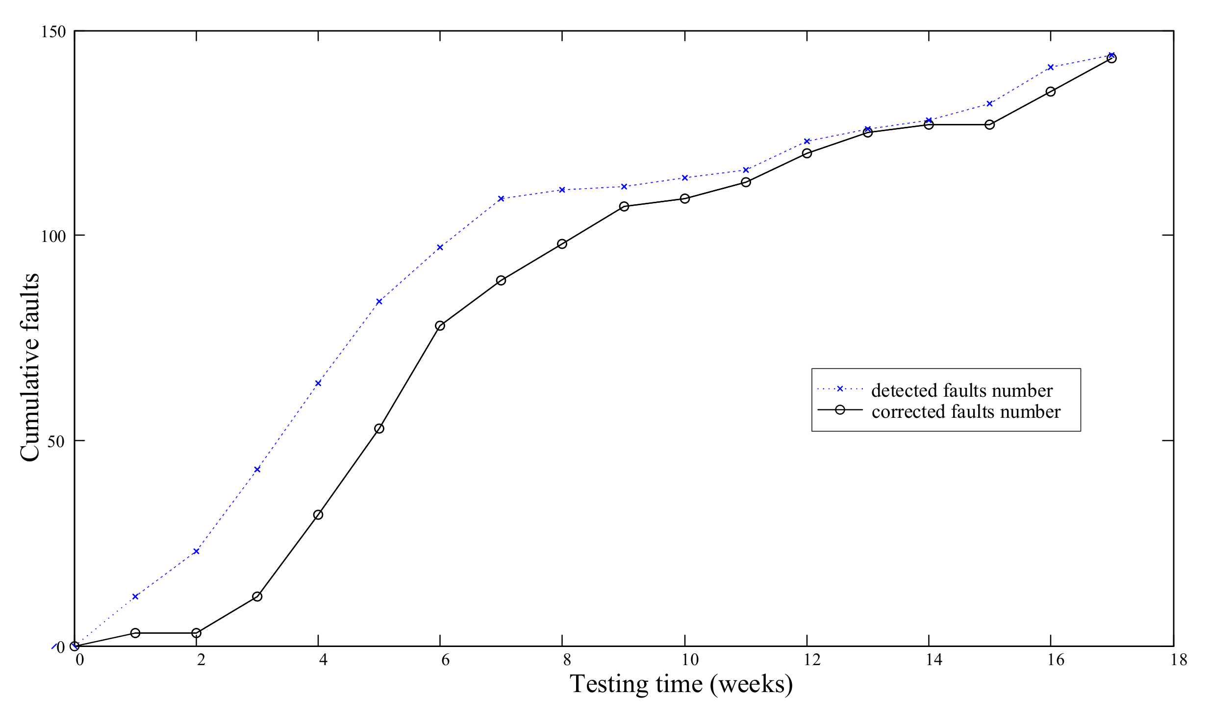
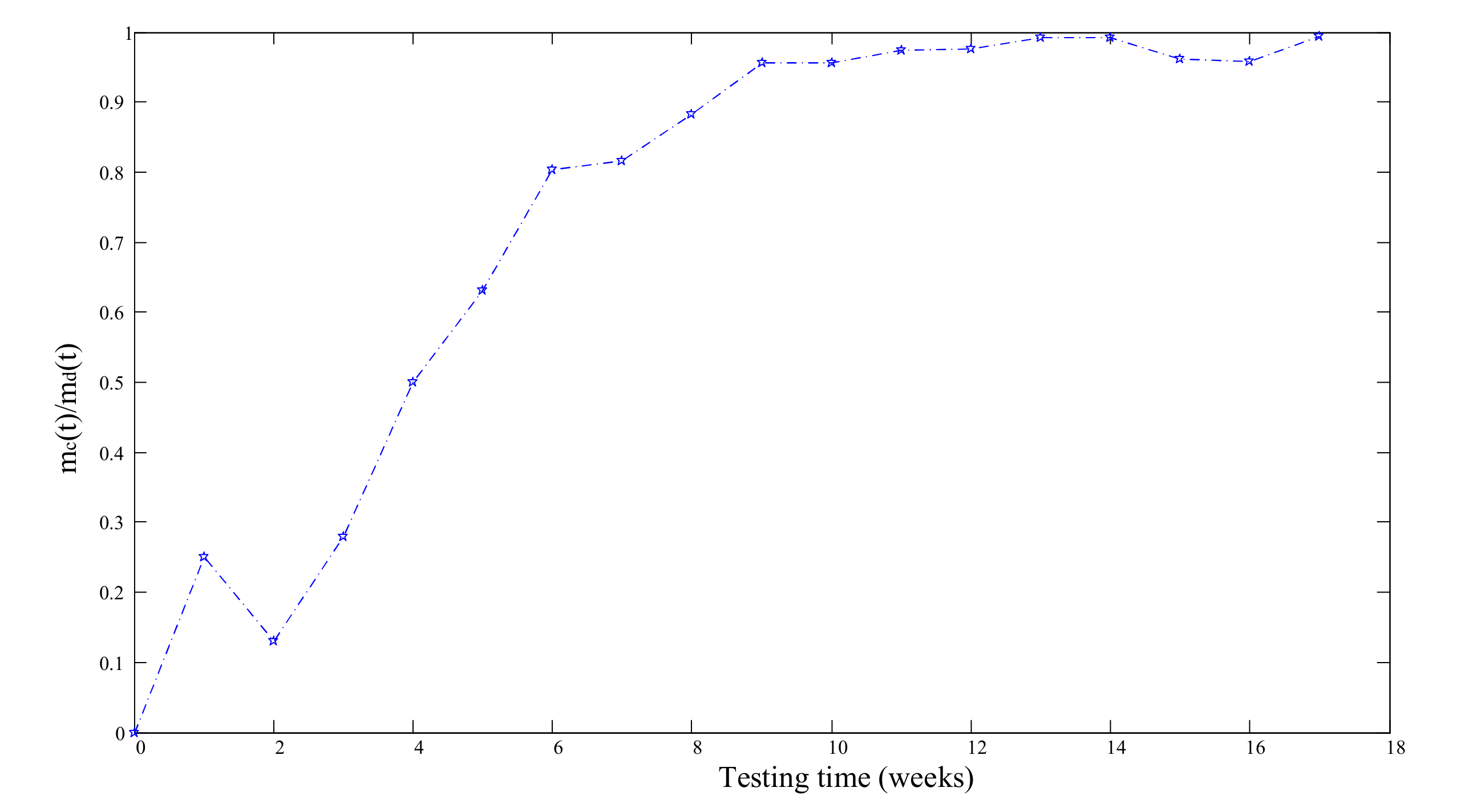
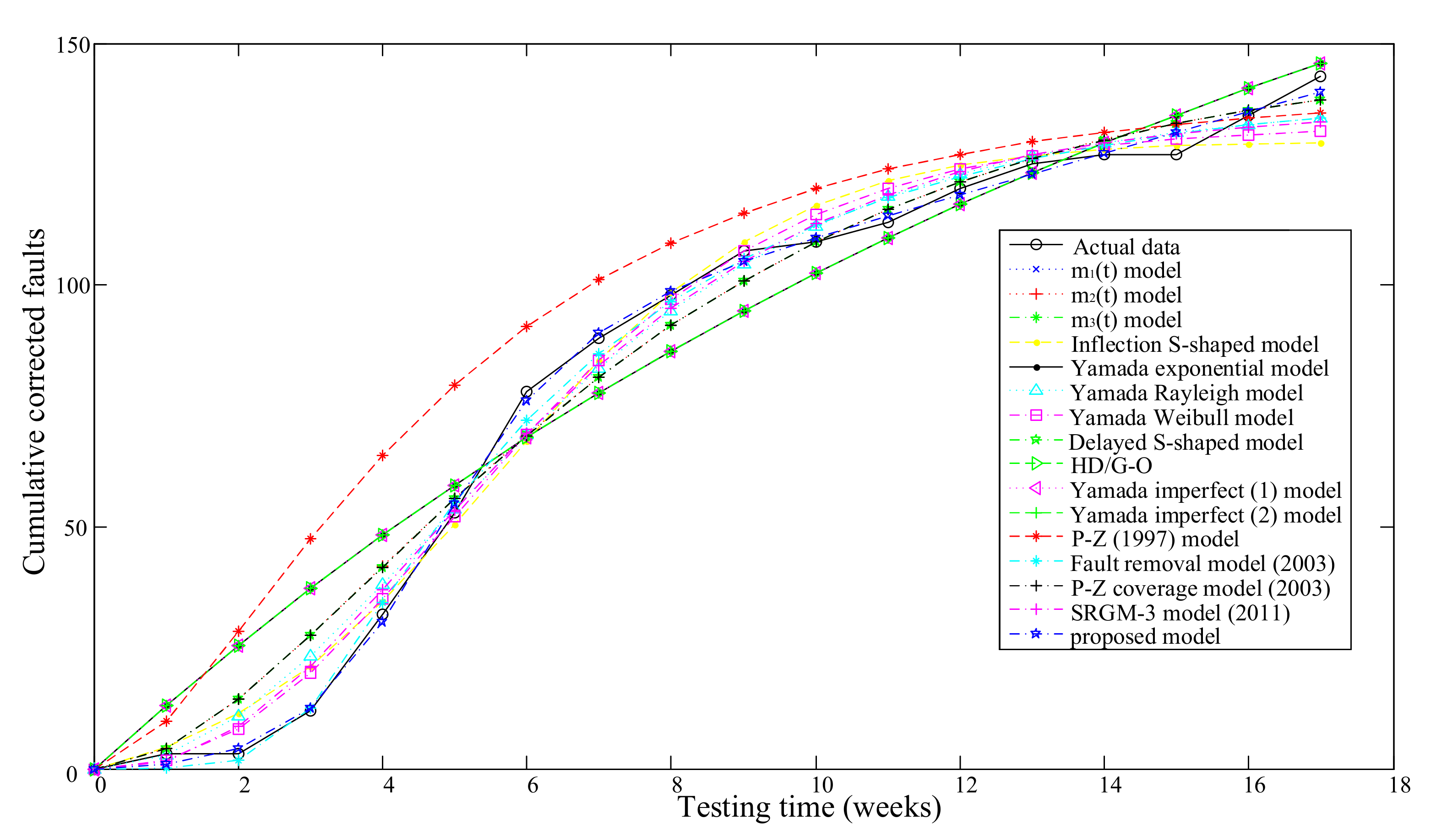
3.2.1. A Middle-Size Software System Data
3.2.2. Monitor and Control System Data
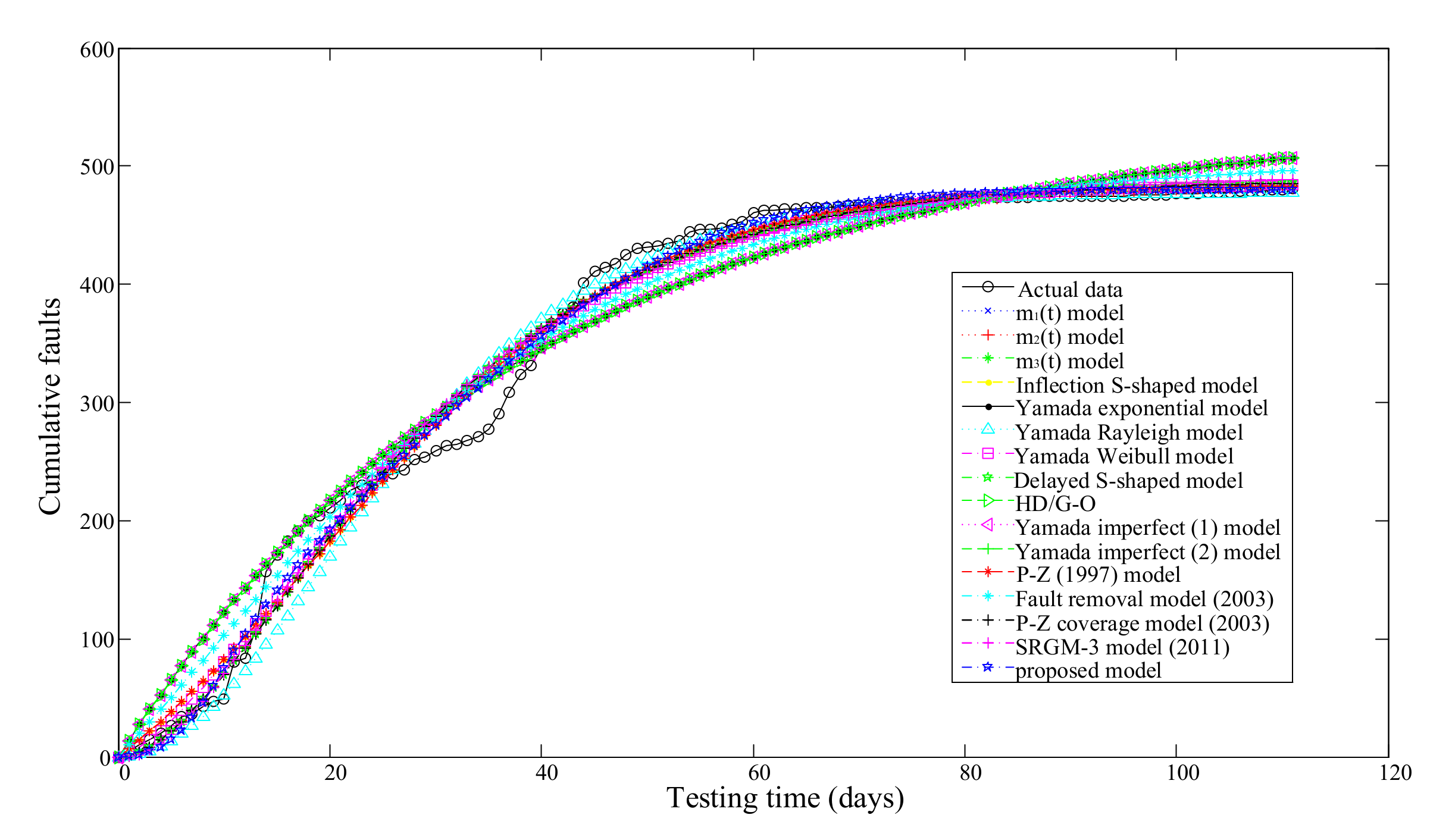
3.2.3. Tandem Computer Data
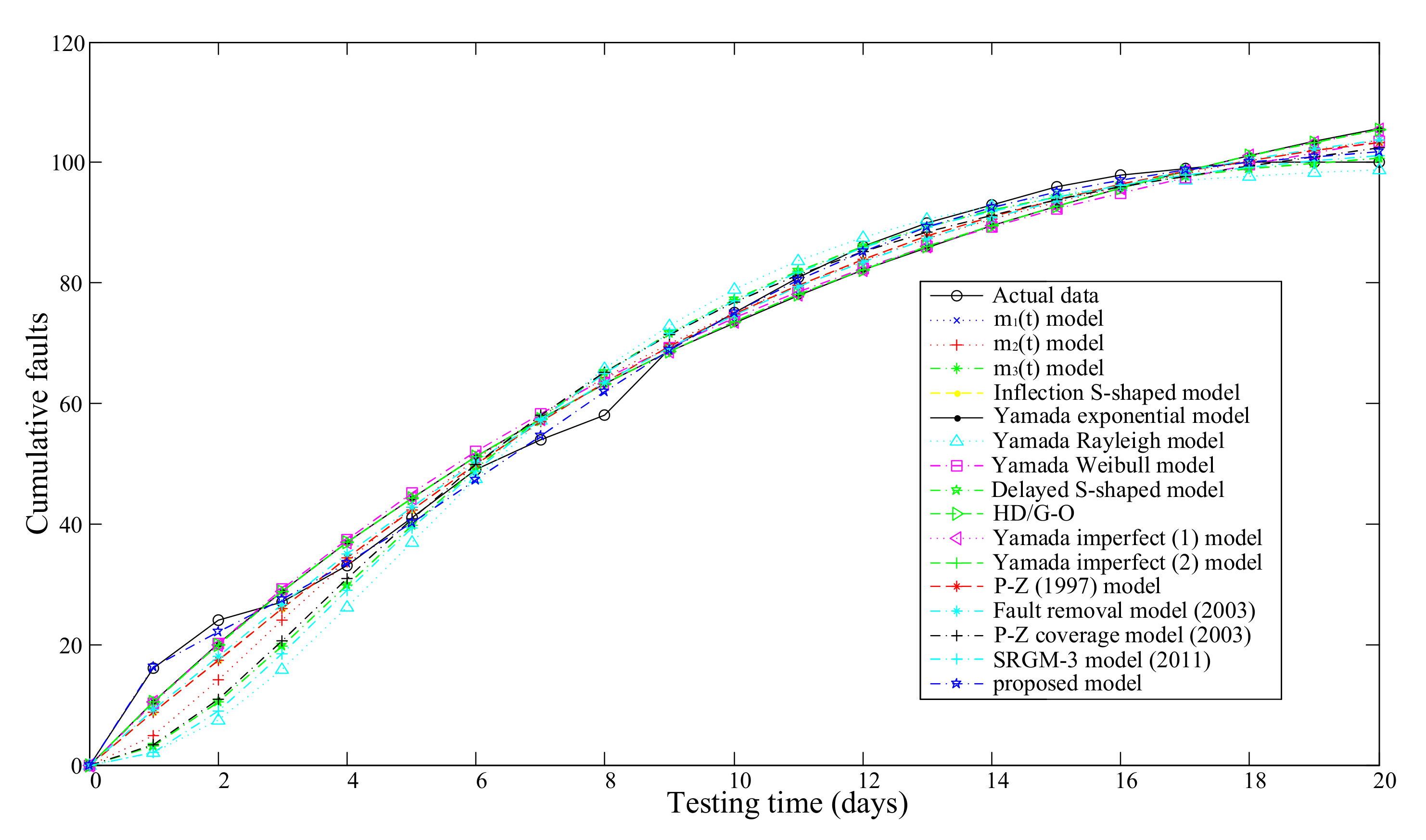
3.2.4. Comparison of Models’ Predictive Power
4. Conclusions
Author Contributions
Funding
Institutional Review Board Statement
Informed Consent Statement
Data Availability Statement
Conflicts of Interest
References
- Erto, P.; Giorgio, M.; Lepore, A. The Generalized Inflection S-Shaped Software Reliability Growth Model. Reliab. IEEE Trans. 2018, 69, 228–244. [Google Scholar] [CrossRef]
- Utkin, L.V.; Coolen, F. A robust weighted SVR-based software reliability growth model. Reliab. Eng. Syst. Saf. 2018, 176, 93–101. [Google Scholar] [CrossRef] [Green Version]
- Saraf, I.; Iqbal, J. Generalized multi-release modelling of software reliability growth models from the perspective of two types of imperfect debugging and change point. Qual. Reliab. Eng. Int. 2019, 35, 2358–2370. [Google Scholar] [CrossRef]
- Jin, C.; Jin, S.W. Parameter optimization of software reliability growth model with S-shaped testing-effort function using improved swarm intelligent optimization. Appl. Soft Comput. 2016, 40, 283–291. [Google Scholar] [CrossRef]
- Pham, H. System Software Reliability; Springer Science and Business Media LLC: Berlin/Heidelberg, Germany, 2006. [Google Scholar]
- Yamada, S.; Tokuno, K.; Osaki, S. Software reliability measurement in imperfect debugging environment and its application. Reliab. Eng. Syst. Saf. 1993, 40, 139–147. [Google Scholar] [CrossRef]
- Huang, C.Y.; Lyu, M.R. Estimation and analysis of some generalized multiple change-point software reliability models. Reliab. IEEE Trans. 2011, 60, 498–514. [Google Scholar] [CrossRef]
- Schneidewind, N.F. Analysis of error processes in computer software. Sigplan Not. 1975, 10, 337–346. [Google Scholar] [CrossRef]
- Xie, M.; Zhao, M. The Schneidewind software reliability model revisited. In Proceedings of the Third International Symposium on Software Reliability Engineering, Research Triangle Park, NC, USA, 7–10 October 1992. [Google Scholar]
- Schneidewind, N.F. Modelling the fault correction process. In Proceedings of the 12th International Symposium on Software Reliability Engineering, Los Alamitos, CA, USA, 27–30 November 2001; pp. 185–190. [Google Scholar]
- Xie, M.; Hu, Q.P.; Wu, Y.P.; Ng, S.H. A study of the modeling and analysis of software fault-detection and fault-correction processes. Qual. Reliab. Eng. Int. 2007, 23, 459–470. [Google Scholar] [CrossRef]
- Wu, Y.P.; Hu, Q.P.; Xie, M.; Ng, S.H. Modeling and analysis of software fault detection and correction process by considering time dependency. Reliab. IEEE Trans. 2007, 56, 629–642. [Google Scholar] [CrossRef]
- Peng, R.; Li, Y.F.; Zhang, W.J.; Hu, Q.P. Testing effort dependent software reliability model for imperfect debugging process considering both detection and correction. Reliab. Eng. Syst. Saf. 2014, 126, 37–43. [Google Scholar] [CrossRef] [Green Version]
- Lo, J.H.; Huang, C.Y. An integration of fault detection and correction processes in software reliability analysis. J. Syst. Softw. 2006, 79, 1312–1323. [Google Scholar] [CrossRef]
- Shuy, J.; Liu, H.W.; Wu, Z.B.; Yang, X.Z. A software reliability growth model integrating fault detection and fault correction processes. Chin. High Technol. Lett. 2010, 20, 386–391. (In Chinese) [Google Scholar]
- Gokhale, S.S.; Lyu, M.R.; Trivedi, K.S. Analysis of Software Fault Removal Policies Using a Non-Homogeneous Continuous Time Markov Chain. Softw. Qual. J. 2004, 12, 211–230. [Google Scholar] [CrossRef]
- Gokhale, S.S.; Lyu, M.R.; Trivedi, K.S. Incorporating fault debugging activities into software reliability models: A simulation approach. Reliab. IEEE Trans. 2006, 55, 281–292. [Google Scholar] [CrossRef]
- Jia, L.; Yang, B.; Guo, S.; Park, D.H. Software reliability modeling considering fault correction process. IEICE Trans. Inf. Syst. 2010, 93, 185–188. [Google Scholar] [CrossRef] [Green Version]
- Huang, C.Y.; Huang, W.C. Software reliability analysis and measurement using finite and infinite server queueing models. Reliab. IEEE Trans. 2008, 57, 192–203. [Google Scholar] [CrossRef]
- Hwang, S.; Pham, H. Quasi-renewal time-delay fault-removal consideration in software reliability modeling. Systems, Man and Cybernetics, Part A: Systems and Humans. IEEE Trans. 2009, 39, 200–209. [Google Scholar]
- Huang, C.Y.; Kuo, S.Y.; Lyu, M.R. An assessment of testing-effort dependent software reliability growth models. Reliab. IEEE Trans. 2007, 56, 198–211. [Google Scholar] [CrossRef]
- Cai, X.; Lyu, M.R. Software Reliability Modeling with Test Coverage: Experimentation and Measurement with A Fault-Tolerant Software Project. 18th IEEE Int. Symp. Softw. Reliab. 2007, 2007, 17–26. [Google Scholar] [CrossRef]
- Malaiya, Y.K.; Li, M.N.; Bieman, J.M.; Karcich, R. Software reliability growth with test coverage. Reliab. IEEE Trans. 2002, 51, 420–426. [Google Scholar] [CrossRef] [Green Version]
- Pham, H.; Zhang, X. NHPP software reliability and cost models with testing coverage. Eur. J. Oper. Res. 2003, 145, 443–454. [Google Scholar] [CrossRef]
- Vouk, M.A. Using Reliability Models during Testing with Non-Operational Profiles. Available online: https://citeseerx.ist.psu.edu/viewdoc/download?doi=10.1.1.47.8863&rep=rep1&type=pdf (accessed on 29 July 2021).
- Gokhale, S.; Trivedi, K.S. A time/structure based software reliability model. Ann. Softw. Eng. 1999, 8, 85–121. [Google Scholar] [CrossRef]
- Park, J.-Y.; Lee, G.; Park, J.H. A class of coverage growth functions and its practical application. J. Korean Stat. Soc. 2008, 37, 241–247. [Google Scholar] [CrossRef]
- Zhang, X.; Teng, X.; Pham, H. Considering fault removal efficiency in software reliability assessment. IEEE Trans. Syst. Man, Cybern. Part A Syst. Hum. 2003, 33, 114–120. [Google Scholar] [CrossRef]
- Ohba, M. Inflection S-Shaped Software Reliability Growth Model; Springer Science and Business Media LLC: Berlin/Heidelberg, Germany, 1984; pp. 144–162. [Google Scholar]
- Yamada, S.; Ohba, M.; Osaki, S. S-shaped reliability growth modeling for software fault detection. Reliab. IEEE Trans. 1983, 12, 475–484. [Google Scholar] [CrossRef]
- Hossain, S.A.; Ram, C.D. Estimating the parameters of a non-homogeneous Poisson process model for software reliability. Reliab.IEEE Trans. 1993, 42, 604–612. [Google Scholar] [CrossRef]
- Yamada, S.; Tokuno, K.; Osaki, S. Imperfect debugging models with fault introduction rate for software reliability assessment. Int. J. Syst. Sci. 1992, 23, 2241–2252. [Google Scholar] [CrossRef]
- Pham, H.; Zhang, X. An NHPP Software Reliability Model and Its Comparison. Int. J. Reliab. Qual. Saf. Eng. 1997, 4, 269–282. [Google Scholar] [CrossRef]
- Kapur, P.K.; Pham, H.; Anand, S.; Yadav, K. A Unified Approach for Developing Software Reliability Growth Models in the Presence of Imperfect Debugging and Error Generation. Reliab. IEEE Trans. 2011, 60, 331–340. [Google Scholar] [CrossRef]
- Tohma, Y.; Yamano, H.; Ohba, M.; Jacoby, R. The estimation of parameters of the hypergeometric distribution and its application to the software reliability growth model. IEEE Trans. Softw. Eng. 1991, 17, 483–489. [Google Scholar] [CrossRef]


| No. | MSE | |||
|---|---|---|---|---|
| 1 | 0.0022 | 0.9765 | 0.9749 | |
| 2 | 0.0038 | 0.9786 | 0.9756 |
| No. | Model Name | Model Type | |
|---|---|---|---|
| 1 | G-O model(also called [14]) | Concave | |
| 2 | [14] | Concave | |
| 3 | [14] | S-shaped | |
| 4 | Inflection S-shaped [29] | Concave | |
| 5 | Yamada exponential [30] | Concave | |
| 6 | Yamada Rayleigh [30] | S-shaped | |
| 7 | Yamada Weibull [30] | Concave and S-shaped | |
| 8 | Delayed S-shaped [30] | S-shaped | |
| 9 | HD/G-O [31] | Concave | |
| 10 | Yamada imperfect (1) [32] | Concave | |
| 11 | Yamada imperfect (2) [32] | Concave | |
| 12 | P-Z(1997) model [33] | S-shaped and Concave | |
| 13 | Fault removal model (2003) [28] | S-shaped | |
| 14 | P-Z coverage model (2003) [24] | S-shaped and Concave | |
| 15 | SRGM-3 model (2011) [34] | S-shaped | |
| 16 | proposed model | S-shaped and Concave |
| Weeks | Cumulative Detected Faults | Cumulative Corrected Faults | Weeks | Cumulative Detected Faults | Cumulative Corrected Faults |
|---|---|---|---|---|---|
| 1 | 12 | 3 | 10 | 114 | 109 |
| 2 | 23 | 3 | 11 | 116 | 113 |
| 3 | 43 | 12 | 12 | 123 | 120 |
| 4 | 64 | 32 | 13 | 126 | 125 |
| 5 | 84 | 53 | 14 | 128 | 127 |
| 6 | 97 | 78 | 15 | 132 | 127 |
| 7 | 109 | 89 | 16 | 141 | 135 |
| 8 | 111 | 98 | 17 | 144 | 143 |
| 9 | 112 | 107 |
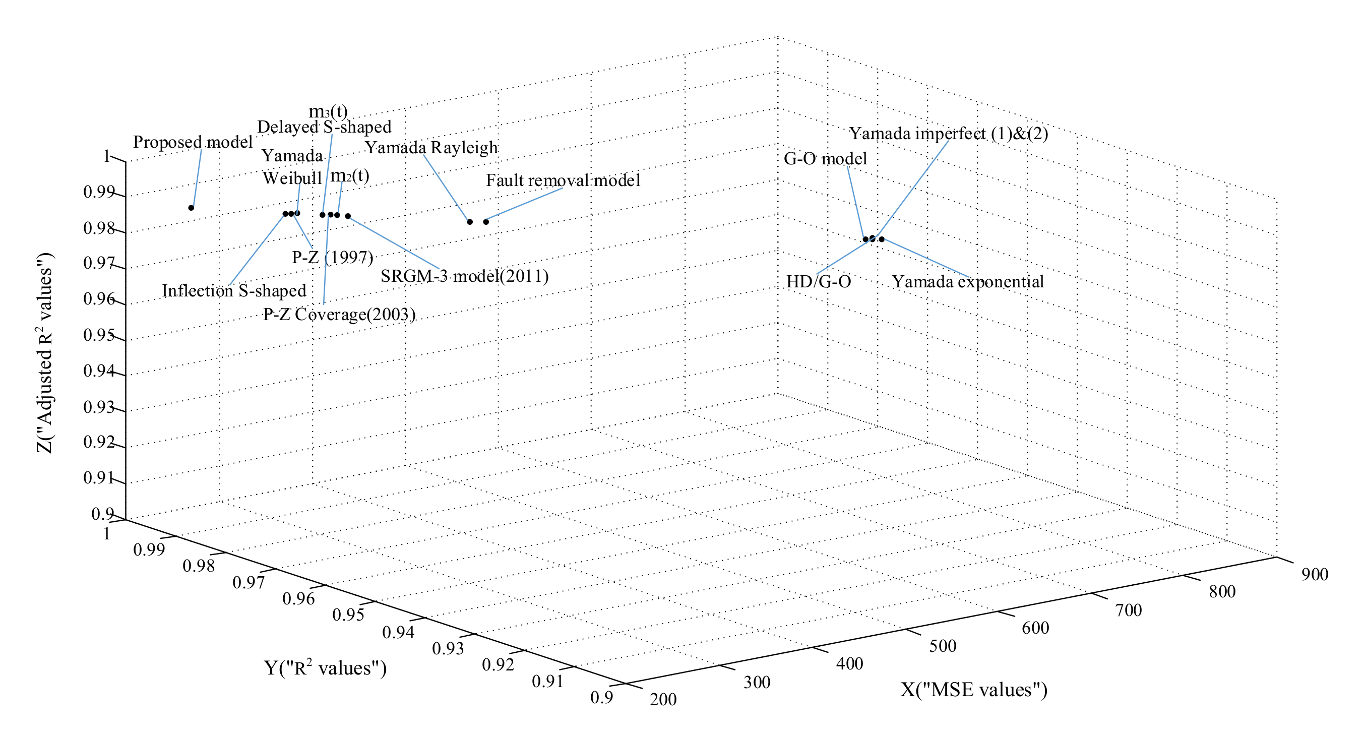
| Model No. | Model Name | Model Parameter Estimation Results | MSE | R2 | Adjusted R2 |
|---|---|---|---|---|---|
| 1 | , | 148.3333 | 0.9396 | 0.9356 | |
| 2 | , , | 56.2357 | 0.9786 | 0.9756 | |
| 3 | , | 52.4867 | 0.9786 | 0.9772 | |
| 4 | Inflection S-shaped | , , | 48.1286 | 0.9817 | 0.9791 |
| 5 | Yamada exponential | , , , | 171.4615 | 0.9395 | 0.9256 |
| 6 | Yamada Rayleigh | , , , | 40.3308 | 0.9858 | 0.9825 |
| 7 | Yamada Weibull | , , , | 34.6385 | 0.9878 | 0.9850 |
| 8 | Delayed S-shaped | , | 52.4867 | 0.9786 | 0.9772 |
| 9 | HD/G-O | , , | 158.9286 | 0.9396 | 0.9310 |
| 10 | Yamada imperfect(1) | , , | 158.9286 | 0.9396 | 0.9356 |
| 11 | Yamada imperfect(2) | , , | 158.9286 | 0.9396 | 0.9356 |
| 12 | P-Z (1997) model | , , , , | 55.7917 | 0.9818 | 0.9758 |
| 13 | Fault removal model (2003) | , , , , , | 19.0364 | 0.9943 | 0.9917 |
| 14 | P-Z coverage model (2003) | , , | 56.2357 | 0.9786 | 0.9772 |
| 15 | SRGM-3 model (2011) | , , , | 34.0154 | 0.9880 | 0.9863 |
| 16 | proposed model | , , , , , | 5.9370 | 0.9984 | 0.9974 |
| Days | Faults | Cumulative Faults | Days | Faults | Cumulative Faults |
|---|---|---|---|---|---|
| 1 | 5 | 5 | 57 | 2 | 448 |
| 2 | 5 | 10 | 58 | 3 | 451 |
| 3 | 5 | 15 | 59 | 2 | 453 |
| 4 | 5 | 20 | 60 | 7 | 460 |
| 5 | 6 | 26 | 61 | 3 | 463 |
| 6 | 8 | 34 | 62 | 0 | 463 |
| 7 | 2 | 36 | 63 | 1 | 464 |
| 8 | 7 | 43 | 64 | 0 | 464 |
| 9 | 4 | 47 | 65 | 1 | 465 |
| 10 | 2 | 49 | 66 | 0 | 465 |
| 11 | 31 | 80 | 67 | 0 | 465 |
| 12 | 4 | 84 | 68 | 1 | 466 |
| 13 | 24 | 108 | 69 | 1 | 467 |
| 14 | 49 | 157 | 70 | 0 | 467 |
| 15 | 14 | 171 | 71 | 0 | 467 |
| 16 | 12 | 183 | 72 | 1 | 468 |
| 17 | 8 | 191 | 73 | 1 | 469 |
| 18 | 9 | 200 | 74 | 0 | 469 |
| 19 | 4 | 204 | 75 | 0 | 469 |
| 20 | 7 | 211 | 76 | 0 | 469 |
| 21 | 6 | 217 | 77 | 1 | 470 |
| 22 | 9 | 226 | 78 | 2 | 472 |
| 23 | 4 | 230 | 79 | 0 | 472 |
| 24 | 4 | 234 | 80 | 1 | 473 |
| 25 | 2 | 236 | 81 | 0 | 473 |
| 26 | 4 | 240 | 82 | 0 | 473 |
| 27 | 3 | 243 | 83 | 0 | 473 |
| 28 | 9 | 252 | 84 | 0 | 473 |
| 29 | 2 | 254 | 85 | 0 | 473 |
| 30 | 5 | 259 | 86 | 0 | 473 |
| 31 | 4 | 263 | 87 | 2 | 475 |
| 32 | 1 | 264 | 88 | 0 | 475 |
| 33 | 4 | 268 | 89 | 0 | 475 |
| 34 | 3 | 271 | 90 | 0 | 475 |
| 35 | 6 | 277 | 91 | 0 | 475 |
| 36 | 13 | 290 | 92 | 0 | 475 |
| 37 | 19 | 309 | 93 | 0 | 475 |
| 38 | 15 | 324 | 94 | 0 | 475 |
| 39 | 7 | 331 | 95 | 0 | 475 |
| 40 | 15 | 346 | 96 | 1 | 476 |
| 41 | 21 | 367 | 97 | 0 | 476 |
| 42 | 8 | 375 | 98 | 0 | 476 |
| 43 | 6 | 381 | 99 | 0 | 476 |
| 44 | 20 | 401 | 100 | 1 | 477 |
| 45 | 10 | 411 | 101 | 0 | 477 |
| 46 | 3 | 414 | 102 | 0 | 477 |
| 47 | 3 | 417 | 103 | 1 | 478 |
| 48 | 8 | 425 | 104 | 0 | 478 |
| 49 | 5 | 430 | 105 | 0 | 478 |
| 50 | 1 | 431 | 106 | 1 | 479 |
| 51 | 2 | 433 | 107 | 0 | 479 |
| 52 | 2 | 435 | 108 | 0 | 479 |
| 53 | 2 | 437 | 109 | 1 | 480 |
| 54 | 7 | 444 | 110 | 0 | 480 |
| 55 | 2 | 446 | 111 | 1 | 481 |
| 56 | 0 | 446 |
| Model No. | Model Name | Model Parameter Estimation Results | MSE | R2 | Adjusted R2 |
|---|---|---|---|---|---|
| 1 | G-O model | , | 804.2202 | 0.9646 | 0.9643 |
| 2 | , , | 338.3333 | 0.9852 | 0.9850 | |
| 3 | , | 331.8349 | 0.9854 | 0.9853 | |
| 4 | Inflection S-shaped | , , | 300.0000 | 0.9869 | 0.9867 |
| 5 | Yamada exponential | , , , | 820.9346 | 0.9645 | 0.9635 |
| 6 | Yamada Rayleigh | , , , | 461.5888 | 0.9800 | 0.9795 |
| 7 | Yamada Weibull | , , , | 308.7850 | 0.9867 | 0.9863 |
| 8 | Delayed S-shaped | , | 331.8349 | 0.9854 | 0.9853 |
| 9 | HD/G-O | , , | 811.6667 | 0.9646 | 0.9639 |
| 10 | Yamada imperfect(1) | , , | 811.6667 | 0.9646 | 0.9643 |
| 11 | Yamada imperfect(2) | , , | 811.6667 | 0.9646 | 0.9643 |
| 12 | P-Z (1997) model | , , , , | 305.6604 | 0.9869 | 0.9864 |
| 13 | Fault removal model (2003) | , , , , , | 419.2381 | 0.9822 | 0.9814 |
| 14 | P-Z coverage model (2003) | , , | 334.9074 | 0.9854 | 0.9853 |
| 15 | SRGM-3 model (2011) | , , , | 354.8598 | 0.9847 | 0.9842 |
| 16 | proposed model | , , , , , | 193.8462 | 0.9919 | 0.9914 |
| Testing Time (Weeks) | CPU (h) | Faults | Cumulative Faults | Testing Time (Weeks) | CPU (h) | Faults | Cumulative Faults |
|---|---|---|---|---|---|---|---|
| 1 | 519 | 16 | 16 | 11 | 6539 | 6 | 81 |
| 2 | 968 | 8 | 24 | 12 | 7083 | 5 | 86 |
| 3 | 1430 | 3 | 27 | 13 | 7487 | 4 | 90 |
| 4 | 1893 | 6 | 33 | 14 | 7846 | 3 | 93 |
| 5 | 2490 | 8 | 41 | 15 | 8205 | 3 | 96 |
| 6 | 3058 | 8 | 49 | 16 | 8564 | 2 | 98 |
| 7 | 3625 | 5 | 54 | 17 | 8923 | 1 | 99 |
| 8 | 4422 | 4 | 58 | 18 | 9282 | 1 | 100 |
| 9 | 5218 | 11 | 69 | 19 | 9641 | 0 | 100 |
| 10 | 5823 | 6 | 75 | 20 | 10,000 | 0 | 100 |
| Model No. | Model Name | Model Parameter Estimation Results | MSE | R2 | Adjusted R2 |
|---|---|---|---|---|---|
| 1 | G-O model | , | 12.9056 | 0.9857 | 0.9849 |
| 2 | , , | 13.6647 | 0.9857 | 0.9840 | |
| 3 | , | 28.0611 | 0.9689 | 0.9672 | |
| 4 | Inflection S-shaped | , , | 10.5647 | 0.9890 | 0.9877 |
| 5 | Yamada exponential | , , , | 14.8438 | 0.9854 | 0.9827 |
| 6 | Yamada Rayleigh | , , , | 49.4188 | 0.9514 | 0.9422 |
| 7 | Yamada Weibull | , , , | 15.1750 | 0.9851 | 0.9823 |
| 8 | Delayed S-shaped | , | 28.0611 | 0.9689 | 0.9672 |
| 9 | HD/G-O | , , | 13.6647 | 0.9857 | 0.9840 |
| 10 | Yamada imperfect(1) | , , | 13.6647 | 0.9857 | 0.9849 |
| 11 | Yamada imperfect(2) | , , | 13.6647 | 0.9857 | 0.9849 |
| 12 | P-Z(1997) model | , , , , | 11.9733 | 0.9890 | 0.9860 |
| 13 | Fault removal model (2003) | , , , , , | 10.8786 | 0.9906 | 0.9873 |
| 14 | P-Z coverage model | , , | 27.1588 | 0.9716 | 0.9683 |
| 15 | SRGM-3 model (2011) | , , , | 14.9250 | 0.9853 | 0.9826 |
| 16 | proposed model | , , , , , | 2.3192 | 0.9981 | 0.9973 |
| Model No. | Model Name | 80% OF DS-1 | 80% OF DS-2 | 80% OF DS-3 |
|---|---|---|---|---|
| SSE | SSE | SSE | ||
| 1 | G-O model(also called ) | 823.0713 | 6.7713 × 10⁴ | 147.2964 |
| 2 | 119.7111 | 7.3709 × 10³ | 356.5743 | |
| 3 | 69.0496 | 3.5343 × 10³ | 6.9655 | |
| 4 | Inflection S-shaped | 750.1803 | 2.7742 × 10³ | 356.5814 |
| 5 | Yamada exponential | 401.7862 | 6.0381 × 10⁴ | 377.2231 |
| 6 | Yamada Rayleigh | 197.3302 | 3.4667 × 10⁵ | 73.4246 |
| 7 | Yamada Weibull | 553.6076 | 3.4596 × 10³ | 676.6515 |
| 8 | Delayed S-shaped | 69.0496 | 3.5343 × 10³ | 6.9655 |
| 9 | HD/G-O | 823.0713 | 6.7713 × 10⁴ | 356.5818 |
| 10 | Yamada imperfect(1) | 823.0770 | 6.7713 × 10⁴ | 356.5837 |
| 11 | Yamada imperfect(2) | 823.0724 | 5.7234 × 10⁴ | 356.5827 |
| 12 | P-Z (1997) model | 595.6770 | 2.8149 × 10³ | 334.1059 |
| 13 | Fault removal model (2003) | 286.2138 | 1.9332 × 10⁴ | 345.1824 |
| 14 | P-Z coverage model (2003) | 69.0496 | 3.5343 × 10³ | 1.5362 × 10³ |
| 15 | SRGM-3 model (2011) | 549.9081 | 1.1495 × 10⁴ | 1.2792 × 10⁴ |
| 16 | proposed model | 37.0169 | 236.0253 | 23.0348 |
Publisher’s Note: MDPI stays neutral with regard to jurisdictional claims in published maps and institutional affiliations. |
© 2021 by the authors. Licensee MDPI, Basel, Switzerland. This article is an open access article distributed under the terms and conditions of the Creative Commons Attribution (CC BY) license (https://creativecommons.org/licenses/by/4.0/).
Share and Cite
Li, Q.; Pham, H. Modeling Software Fault-Detection and Fault-Correction Processes by Considering the Dependencies between Fault Amounts. Appl. Sci. 2021, 11, 6998. https://doi.org/10.3390/app11156998
Li Q, Pham H. Modeling Software Fault-Detection and Fault-Correction Processes by Considering the Dependencies between Fault Amounts. Applied Sciences. 2021; 11(15):6998. https://doi.org/10.3390/app11156998
Chicago/Turabian StyleLi, Qiuying, and Hoang Pham. 2021. "Modeling Software Fault-Detection and Fault-Correction Processes by Considering the Dependencies between Fault Amounts" Applied Sciences 11, no. 15: 6998. https://doi.org/10.3390/app11156998
APA StyleLi, Q., & Pham, H. (2021). Modeling Software Fault-Detection and Fault-Correction Processes by Considering the Dependencies between Fault Amounts. Applied Sciences, 11(15), 6998. https://doi.org/10.3390/app11156998