An Ensemble Feature Selection Approach to Identify Relevant Features from EEG Signals

Abstract

Identifying relevant data to support the automatic analysis of electroencephalograms (EEG) has become a challenge. Although there are many proposals to support the diagnosis of neurological pathologies, the current challenge is to improve the reliability of the tools to classify or detect abnormalities. In this study, we used an ensemble feature selection approach to integrate the advantages of several feature selection algorithms to improve the identification of the characteristics with high power of differentiation in the classification of normal and abnormal EEG signals. Discrimination was evaluated using several classifiers, i.e., decision tree, logistic regression, random forest, and Support Vecctor Machine (SVM); furthermore, performance was assessed by accuracy, specificity, and sensitivity metrics. The evaluation results showed that Ensemble Feature Selection (EFS) is a helpful tool to select relevant features from the EEGs. Thus, the stability calculated for the EFS method proposed was almost perfect in most of the cases evaluated. Moreover, the assessed classifiers evidenced that the models improved in performance when trained with the EFS approach’s features. In addition, the classifier of epileptiform events built using the features selected by the EFS method achieved an accuracy, sensitivity, and specificity of 97.64%, 96.78%, and 97.95%, respectively; finally, the stability of the EFS method evidenced a reliable subset of relevant features. Moreover, the accuracy, sensitivity, and specificity of the EEG detector are equal to or greater than the values reported in the literature.

1. Introduction

Research on developing systems for capturing and analyzing biomedical signals has increased over time [1]. In addition, the need to find new mechanisms to support the clinical diagnosis of specific pathologies has accelerated this process. For instance, electroencephalographic (EEG) signal processing monitors neuronal activity in the brain and obtains data that describe valuable information for detecting neurological pathologies. Nowadays, the diagnosis of diseases such as epilepsy through digital analysis of EEG signals has become one of the promising research areas supporting the automatic EEG reading [2]. The EEG signals are decomposed and processed through feature extraction mechanisms to obtain a description that can classify them as normal or abnormal [3]. Likewise, other studies based on the analysis of EEG signals have been performed to analyze brain activity [4,5] and support clinical diagnosis. For example, some proposals have used neural networks, decision trees, rules based on domain knowledge, and clustering mechanisms to classify new signals [6,7].

Even though numerous mechanisms characterize EEG signals by detecting or classifying events associated with epilepsy, this area’s most significant research challenge is improving the classification’s performance in terms of precision, accuracy, and recall, providing reliable tools that support neurologists in the diagnosis. Considering the above, one of the main strategies to improve the classification models in machine learning or data mining is to train the models with relevant features, that is, those features that do not represent noise for the learning model and, on the contrary, have a high power of differentiation between classes.

On the other hand, feature selection (FS) helps build robust classification models [8] by identifying relevant features. This process is a mandatory task, especially when the datasets have (i) high dimensionality [7] or (ii) more features than instances, which means the dataset has more columns than rows. This scenario coincides with the classification of abnormalities in EEGs considering the large number of feature extractors reported in the literature and the low availability of datasets with instances or single rows that describe epileptiform events.

Besides, the literature review shows the use of different feature selection techniques to support the automatic analysis of different types of physiological signals. For example, proposals range from general methods to select features on clinical databases [9] to implementations designed to help the diagnosis of diseases such as Alzheimer’s [10], multiple sclerosis [11], sleep disorders [12], and epilepsy [13]. Additionally, the list of reviewed papers presents solutions designed for the detection of emotions by analyzing the electrical activity of the brain [14] or the recognition of activities using analysis of physiological signals [15] and external devices [16]. Furthermore, some literature has reported feature selection methods to identify features with the more remarkable power of differentiation in classifying or detecting epileptic patterns. However, most of the reviewed results focused on identifying specific patterns using a set of features without considering each feature’s relevance or impact in subsequent analyses [6]. Thus, the proposals end up training machine learning models with features that could represent noise or redundancy for the learning process.

Recently, several studies have focused on improving the performance of feature selection algorithms. For example, in [17], the authors proposed identifying correlations between features and classes to enhance the effectiveness and maintain a low computational cost in the feature selection process. Additionally, Refs. [18,19] incorporated techniques such as bootstrap to select features using samples from the original dataset and integrate the subsets of features generated. However, these proposals depend on balancing the datasets and the continuous data (data that can be measured on an infinite scale), which could bias the subsequent analyses. Hence, some authors have proposed assembly feature selection algorithms to improve the identification of relevant features through the consensus of FS algorithms with different approaches [20].

Considering the above, we believe that an ensemble feature selection (EFS) approach can improve the selection of relevant features and enhance the classification of epileptiform events in EEG signals. Furthermore, this approach is based on the premise of multiple classifiers: “several classifiers classify better than one”, which would be applied to the feature selection, where we intended to demonstrate that “several feature selectors select better than one”.

The main objective of this paper is to show how to improve the classification of EEG signals by enhancing the feature selection process with the ensemble feature selection method.

The rest of the document is organized as follows: Section 2 shows the feature extractors used to calculate the dataset of normal and abnormal segments of EEGs. Section 3 presents the evaluation performed to validate the relevant features selected by the EFS approach. Section 4 offers a discussion of results and contributions. Finally, Section 5 describes the main conclusions of this research.

2. Materials and Methods

2.1. Dataset

The EEG repository built in [21] contains 200 records from 200 patients that, given their structure, cannot be processed by machine learning algorithms. Each EEG record was acquired under the electrode positioning system 10–20, considering a sampling rate of 200 samples per second for 21 channels and an approximate duration of 30 min. The 200 EEG records were diagnosed by a pediatric neurologist with 20 years of experience reading this kind of exam.

Besides, each EEG was decomposed channel by channel, and 672 segments diagnosed as abnormal were extracted and described using a set of feature extractors. Each segment had 200 samples. This same process was carried out for a set of 672 segments considered normal. Thus, the dataset was built with 142 features extracted from 1344 EEG segments. Since all the descriptors were applied to all the segments, the dataset did not contain columns with null data.

The descriptors used to extract the features from the EEG signals are described below.

• Basic Descriptors

Statistical features allow summarizing the values that describe a segment of EEG signal in a single value. The measures of this type that will be applied in the construction of the dataset are min, max, mean, median, low median, high median, variance, and standard deviation.

• Entropy

Entropy is considered a family of statistical measures that quantify the variant complexity in a system. In this study, we evaluated three different ways of measuring Entropy:

○

Shannon Entropy

$$H_{\alpha }\left(\phi \right)=\frac{1}{1-\alpha }{\mathit{log}}_2\{\frac{{\sum }_{k=1}^n{P}_k^{\alpha }}{{\sum }_{k=1}^{n}Pk}$$

(1)

○

Approximate Entropy

$$\mathrm{ApEn}\left(m,r,N\right)={\varnothing }^m\left(r\right)-{\varnothing }^{m+1}\left(r\right)$$

(2)

○

Renyi Entropy

$$\mathrm{RenyiEntropy}\left(x,m\right)=\mathrm{SamEn}\left(x,m,r\right)+log\left(2r\right)$$

(3)

• Kurtosis and Skewness
  The skewness and kurtosis are higher-order statistical attributes of a time series.

  ○

  Skewness represents the degree of distortion from the symmetrical bell curve or the normal distribution. In other words, the lack of symmetry in data distribution is measured by skewness.

  ○

  Kurtosis measures the peakedness of the probability density function (PDF) of a time series. It is used to measure the outliers present in the distribution.

• Energy

The signal is viewed as a function of time, and energy represents its size. The energy can be measured in different ways, but the area under the curve is the most common measure to describe the size of a signal. It measures the signal strength, and this concept can be applied to any signal or vector.

$$E_x=\underset{-\infty }{\overset{\infty }{{\displaystyle \int }}}{\left|\mathrm{x}\left(t\right)\right|}^{2}dt$$

(4)

• Fractal Dimension—Higuchi

The fractal dimension corresponds to a noninteger dimension of a geometric object. Based on this principle, fractal dimension analysis is used to analyze biomedical signals. In this approach, the waveform is considered a geometric figure [22].

$$D=\frac{d\mathit{log}\left(L\left(k\right)\right)}{d\mathit{log}\left(k\right)}$$

(5)

• Fractal Dimension—Petrosian

This type of analysis provides a quick mechanism to calculate the fractal dimension bypassing the series in a binary sequence. For example, the following describes the equation that calculates the Petrosian fractal dimension [22]:

$$F_{Petrosian}=\frac{lo{g}_{10}\left(n\right)}{lo{g}_{10}\left(n\right)+{\mathit{log}}_{10}(\frac{n}{n+0.4N_{∆}})}$$

(6)

• Hurst Exponent

This exponent is a measure of the predictability of the signal. It is a scalar between 0 and 1 which measures long-range correlations of a time series [23].

• Zero-Crossing Rate

The zero-crossing rate is a statistical feature that describes the number of times that a signal crosses the horizontal axis.

• Hjort Parameters

The Hjort parameters describe statistical properties in the time domain [12]. Usually, these are used to analyze electroencephalography signals.

○

Activity

Activity, also known as the variance or mean power, measures the squared standard deviation of the amplitude.

$$\mathrm{Activity}=\frac{{{\displaystyle \int }}_{n-1}^{Nn}\left(x\left(n\right)-\overline{x}\right)}{N}$$

(7)

○

Mobility

Mobility measures the standard deviation of the slope concerning the standard deviation of the amplitude.

$$\mathrm{Mobility}\left(x\right)=\sqrt{\frac{\mathrm{var} \left(x^{\prime }\right)}{\mathrm{var}\left(x\right)}}$$

(8)

○

Complexity

This parameter is associated with the wave shape.

$$\mathrm{Complexity}\left(x\right)=\frac{\mathrm{Mobility}\left(x^{\prime }\right)}{\mathrm{Mobility}\left(x\right)}$$

(9)

• Discrete Wavelet Transform

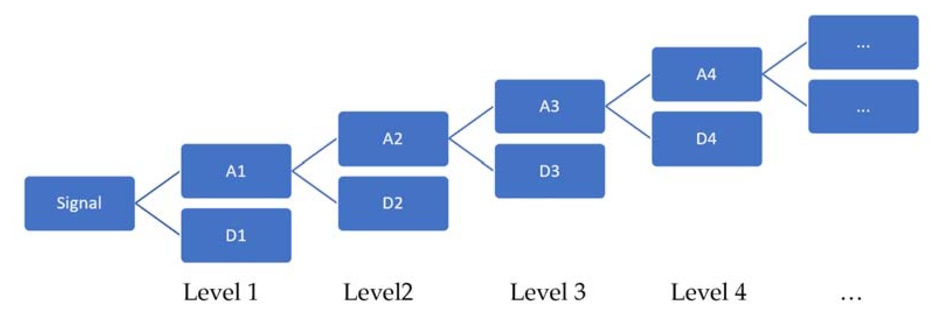
The discrete wavelet transform allows the analysis of a signal in a specific segment. The procedure consists of expressing a continuous signal to expand coefficients of the internal product between the particular segment and a mother wavelet function. As a result, the wavelet transform’s discretization changes from a continuous mapping to a finite set of values. This process is done by changing the integral in the definition by an approximation with summations. Hence, the discretization represents the signal in terms of elementary functions accompanied by coefficients.

$$f\left(t\right)={\displaystyle \sum }_{\lambda }{c}_{\lambda }{\phi }_{\lambda }$$

(10)

The mother wavelet functions include a set of scale functions. The parent functions represent the fine details of the signal, while the scale functions calculate an approximation. Thus, considering the above, a function or signal can be described as a summation of wavelet functions and scale functions.

$$f\left(t\right)={\sum }_k{\sum }_j{c}_{j,k}\varnothing \left(t\right)+{\sum }_k{\sum }_j{d}_{j,k}\psi \left(t\right)$$

(11)

A signal can be decomposed into various levels from the time domain to the frequency domain in wavelet analysis. The decomposition is done from the detail coefficients as well as the approximation coefficients. Figure 1 describes the different encoding paths for n levels of decomposition. The upper level of the tree represents the temporal representation. As the decomposition levels increase, an increase in the compensation in the time–frequency resolution is obtained. Finally, the last level of the tree describes the representation of the signal frequency.

• Fast Fourier Transform

The fast Fourier transform computes a short version of the discrete Fourier transform of a signal by decomposing the original signal into different frequencies (smaller transforms). The decomposed signals are used to calculate the resulting transform signal. FFT is used to convert a signal from the time domain to a representation in the frequency domain or vice versa.

Features extracted from the fast Fourier transform calculation are as follows:

○

Spectral Centroid

The spectral centroid is a statistical measure used to describe the spectrum’s shape in digital signal processing. This centroid defines the spectrum as a probability distribution and represents where the center of mass of the spectrum is located.

$$\mathrm{Centroid}=\frac{{\sum }_{n=0}^{N-1}f\left(n\right)x\left(n\right)}{{\sum }_{n=0}^{N-1}x\left(n\right)}$$

(12)

○

Spectral Flatness

The Spectral Flatness defines the ratio of the geometric mean to the arithmetic mean of a power spectrum.

$$\mathrm{Flatness}=N\frac{\sqrt[N]{{\prod }_{n=0}^{N-1}x\left(n\right)}}{\frac{{\sum }_{n-0}^{N-1}x\left(n\right)}{N}}=\frac{\exp \left(\frac{1}{N}{\sum }_{n=0}^{N-1}\ln x(n\right)}{\frac{1}{N}{\sum }_{n=0}^{N-1}x\left(n\right)}$$

(13)

○

Crest Factor

The crest factor defines how extreme the peaks are in a signal.

$$C=\frac{\left|x_{peak}\right|}{x_{rms}}=\frac{{\left|\left|x\right|\right|}_{\infty }}{{\left|\left|x\right|\right|}_2}$$

(14)

• Matched Filter

Matched filters are basic signal analysis tools used to extract known waveforms from a signal that has been contaminated with noise. For example, in the context of the detection of epileptic spikes, given a signal $x\left(t\right)$ that describes the brain activity (EEG), the matched filter $h\left(t\right)$ seeks a well-known pattern of epilepsy s(t); then, if the signal contains an epileptiform pattern, the signal is described by the brain activity $n\left(t\right)$ with the abnormality $s\left(t\right)$ generating $x\left(t\right)=s\left(t\right)+n\left(t\right).$ Otherwise, the signal only contains the normal brain activity $x\left(t\right)=n\left(t\right).$

Considering the above, 21 descriptors were applied on the normal and abnormal EEG segments, and their wavelet coefficients (5) were generated from the original segments generating 126 features. The 21 descriptors are min, max, mean, median, high median, low median, variance, standard deviation, Shannon entropy, approximate entropy, Renyi entropy, kurtosis, skewness, energy, Higuchi fractal dimension, Petrosian fractal dimension, Hurst exponent, zero-crossing rate, Hjort activity, Hjort mobility, and Hjort complexity. Besides, the fast Fourier transform (FFT) was calculated, and 15 descriptors were applied to the result of FFT: min, max, mean, median, high median, low median, variance, standard deviation, Shannon entropy, kurtosis, skewness, energy, spectral centroid, spectral flatness, and crest factor. The matched filter was also applied to the original segments, and a Boolean feature was generated with the results. Then, we obtained 142 features: 126 features calculated from the original segment and 5 wavelet coefficients (21 × 6), 15 features extracted from the FFT calculation, and the matched filter.

Considering the number of segments that could be analyzed in a single EEG record (1 EEG with 21 channels and 30 min of duration could generate more than 37,800 segments of 200 samples), it is necessary to reduce the number of features not only to reduce the complexity of describing the segments but also to avoid the introduction of noise and redundant information into the classification process and increase the stability of the classifiers.

2.2. The Ensemble Feature Selection Approach

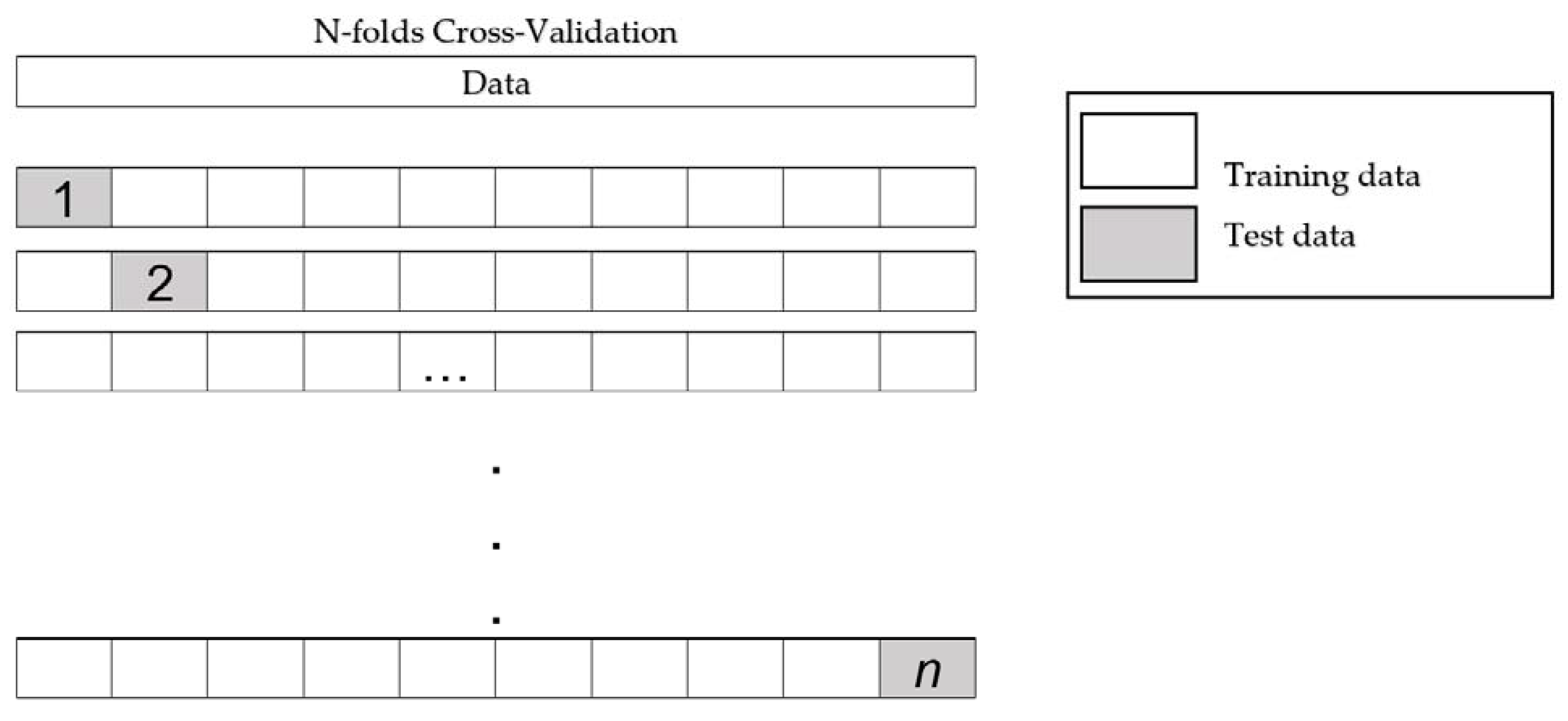
A dataset could contain three types of features: relevant, redundant, and noise. The category of the feature selection (FS) method: filter, wrapper, or embedded, is defined by the mechanism that evaluates the relevance of the features: statistical tests or cross-validation. The analysis performed by FS methods defines a ranking of feature relevance in the filter-based techniques, a subset of relevant features in wrapper methods, or a subset of features with a learning model in the embedded methods. The rankings of features generated by filter methods are used to select the k highest-ranked features.

Considering ensemble learning, the consensus of several experts improves the creation of a decision in a context [24]. Thus, we decided to use the results of our previous research, where we built a framework of ensemble feature selection [25]. This considers the pooling of n FS algorithms by aggregating their results in a unique subset of relevant features. This scheme is described in Figure 2 and defined in [26] as a heterogeneous centralized ensemble, where single methods represent each FS method used to select a subset of relevant features, outcomes of single methods are the subset generated, pooling is the process to aggregate all subsets of relevant features, and relevant features are the result of the pooling process.

The EFS method described in [25] uses an importance index (II) to aggregate the subsets generated by the n FS algorithms. First, the subsets of features generated by each FS method build a set SUM with all selected features. Then, for each feature in the subset SUM, the importance index is computed according to Equation (15). Thus, the number of times that feature i is presented in the subset SUM ($F{F}_i$) is divided by n to calculate its importance index. Finally, the EFS selects the features with an importance index greater than a threshold defined by the user.

$$I{F}_i=\frac{F{F}_i}{n }$$

(15)

The main objective of the ensemble feature selection approach is to reach a consensus among several FS methods to generate a subset of relevant features capable of representing the advantages of all used methods and face the biases of the single methods by compensating their disadvantages with the benefits of the others. Thereby, the result of EFS is a subset of relevant features that could improve the performance of subsequent analyses, such as classification processes.

Although the EFS implemented in the framework could be configured with different FS algorithms, in this study, we used five FS algorithms, three based on rankings of features (ANOVA, chi-squared, and mutual information), one wrapper (importance of features calculated by decision trees), and one embedded (recursive feature elimination—RFE). Each single FS algorithm generated a subset of relevant features, which the EFS aggregates.

2.3. N-Fold: Cross-Validation

Cross-validation is an analysis tool that allows the evaluation of the results offered by a model. This method is used to divide the dataset into smaller sets to train and evaluate a classifier. The single step divides a sample into test and training data. For this study, the application of single cross-validation was carried out for splitting the test data. However, N-fold cross-validation implied breaking the original dataset into n samples, and for each sample, it tested and trained the subsamples. Averaging accuracies calculated for all samples allowed us to determine a general accuracy statistically.

Figure 3 describes a general scheme of N-fold cross-validation. It shows how the mechanism divides the sample data into n partitions and performs the traditional cross-validation process n times, iterating different partitions as a test dataset and the remaining n − 1 partitions as a training dataset.

2.4. Classification Algorithms

In machine learning, classification is a process for categorizing data into classes. The objective is to predict the class of given data points or instances. For this study, we implemented the following algorithms using the scikit-learn framework:

• Decision Tree: This is supervised machine learning algorithm where the data are divided into several levels to obtain an outcome (class). For the evaluation, the algorithm’s parameters were tested to evaluate the best performance for the classification. However, the best results were achieved when the entropy of the value and random were assigned to the parameters criterion and splitter.
• Logistic Regression: This is a machine learning algorithm for binary classification. This method measures the relationship between the variable that we want to predict and the features by estimating probabilities. One of the parameters established in the configuration was class_weight to define if the dataset was balanced or not. Besides, the solver used was liblinear to minimize the multivariate function by solving the univariate optimization problem in a loop.
• Random Forest: This is a machine learning algorithm based on the ensemble of decision trees. The configuration of this algorithm that achieved the best performance of the model included 35 estimators, entropy as a function to measure the quality of a split (criterion), and bootstrap option.
• Support Vector Machine: This is a popular supervised learning algorithm; its goal is to create the best line (decision) boundary to segregate n-dimensional space into classes. We used a kernel polynomial with 3 degrees and without a limit of iterations for building the SVM classifier.

All settings were made according to the scikit-learn configurations.

2.5. Jackar Index

The Jackar index is a statistic used to measure the similarities between sample sets. It is defined by Equation (16):

$$J\left(A,B\right)=\frac{\left|A {\displaystyle \cap } B\right|}{\left|A {\displaystyle \cup } B\right|}$$

(16)

A and B are two subsets of relevant features calculated by an FS algorithm using different data samples.

2.6. The Detector of Epileptic Activity

Figure 4 describes an architecture proposal of a detector of epileptic events. In this scheme, the detector decomposes an EEG signal into channels and segments. Thus, each channel was broken into 200 samples, and each segment was classified as normal or abnormal using a classifier.

3. Results

The evaluation was divided into three stages. The first one focused on assessing the feature relevance; thus, we compared the performance of several classification algorithms using all features with the performance achieved when we used subsets of relevant features selected by the EFS approach. The second stage evaluated the classification algorithm and the subset of relevant features that reached the best performance in the previous step by applying N-fold cross-validation. Finally, the stability of the subset of relevant features was calculated.

3.1. Evaluating Ensemble Feature Selection (EFS)

To evaluate the utility of subset features selected by the EFS algorithm, a set of four classifiers (decision tree, logistic regression, random forest, and SVM) were configured to determine which one of them achieves the best performance in classifying normal or abnormal brain activity. The evaluation considered 70% of data for training the models and 30% for testing them. This process was repeated 10 times, and the data were split randomly.

Table 1. Accuracy results—decision tree classifier.

K	Features Selected	Decision Tree Classifier
		All	EFS
1	3	95.97 ± 1.4	92.03 ± 1.8
3	10	95.91 ± 1.5	93.82 ± 1.5
5	17	95.71 ± 1.6	94.48 ± 2.1
7	23	95.78 ± 1.4	95.08 ± 1.9
9	27	95.90 ± 1.01	96.02 ± 1.03
15	35	95.97 ± 1.21	96.12 ± 1.01

,

Table 2. Accuracy results—logistic regression.

K	Features Selected	Logistic Regression
		All	EFS
1	3	97.17 ± 0.98	90.31 ± 1.8
3	10	97.37 ± 1.1	91.89 ± 3.1
5	17	97.31 ± 1.6	92.27 ± 3.0
7	23	97.39 ± 1.2	95.16 ± 2.1
9	27	97.02 ± 1.4	95.08 ± 1.6
15	35	97.24 ± 1.32	95.28 ± 1.54

,

Table 3. Accuracy results—random forest.

K	Features Selected	Random Forest
		All	EFS
1	3	89.17 ± 2.2	87.84 ± 2.03
3	10	89.2 ± 2.76	88.17 ± 3.13
5	17	89.32 ± 2.6	88.79 ± 2.6
7	23	89.24 ± 2.7	89.24 ± 2.26
9	27	89.31 ± 2.8	89.72 ± 2.6
15	35	89.45 ± 2.12	89.81 ± 2.57

and

Table 4. Accuracy results—SVM.

K	Features Selected	SVM
		All	EFS
1	3	87.69 ± 1.17	94.63 ± 1.5
3	10	87.54 ± 1.15	94.93 ± 1.4
5	17	87.61 ± 1.2	95.97 ± 1.2
7	23	87.69 ± 1.07	96.61 ± 1.07
9	27	87.29 ± 1.2	96.79 ± 1.05
15	35	87.06 ± 1.2	97.31 ± 1.01

describe the results of the accuracy and standard deviation of accuracy in classification calculated using all features and the subset of selected features by the EFS technique using different sizes (K) of the subsets generated by the single methods. “Features selected” represents the number of features chosen after aggregating the subsets generated by each FS algorithm in the EFS method. Thus, K represents the number of features determined by each FS algorithm. Besides, when we trained the models with all features, we obtained different values in each row because we repeated each EFS test. However, although the values are different, they are close. These results are because the data were randomly split in each test, and each test used different samples of the data.

Table 1, Table 2, Table 3 and Table 4 prove that subsets of selected features could reach a similar performance in classification compared to the performance achieved using all features. Even the accuracy of SVM improved when the classification process used only subsets of features selected by the EFS technique. Likewise, the previous tables show that support vector machine was the algorithm with the best performance in classifying abnormal and normal segments of brain activity.

Table 5. Subsets of features selected by single algorithms.

Algorithm	Subset
SelectKBest1	‘F11’, ‘F15’, ‘F28’, ‘F32’, ‘F36’, ‘F40’, ‘F49’, ‘F53’, ‘F57’, ‘F61’, ‘F70’, ‘F74’, ‘F78’, ‘F95’, ‘F99’
SelectKBest2	‘F1’, ‘F55’, ‘F60’, ‘F65’, ‘F71’, ‘F76’, ‘F77’, ‘F85’, ‘F86’, ‘F92’, ‘F97’, ‘F106’, ‘F118’, ‘F126’, ‘F132’
SelectKbest3	‘F1’, ‘F55’, ‘F60’, ‘F65’, ‘F71’, ‘F76’, ‘F77’, ‘F85’, ‘F86’, ‘F92’, ‘F97’, ‘F106’, ‘F118’, ‘F126’, ‘F132’
RFE	‘F11’, ‘F15’, ‘F28’, ‘F32’, ‘F36’, ‘F53’, ‘F70’, ‘F74’, ‘F78’, ‘F95’, ‘F99’, ‘F116’, ‘F120’, ‘F140’, ‘F141’
Feature Importance	‘F97’, ‘F76’, ‘F92’, ‘F118’, ‘F85’, ‘F114’, ‘F126’, ‘F77’, ‘F107’, ‘F119’, ‘F106’, ‘F18’, ‘F86’, ‘F65’, ‘F64’

shows the features selected by each single FS algorithm that allowed training the model with the best performance in this preliminary test.

The select K best FS methods were calculated using the ANOVA, chi-squared, and mutual information metrics.

3.2. Selecting Relevant Features from the EEG Dataset

This phase used EFS to analyze the relevance of features on a dataset with descriptions of normal and abnormal segments extracted from EEGs. To validate the subset of relevant features calculated using the EFS method, a classification process was built to evaluate the accuracy reached with the subset of features selected.

The setting of the aggregation method of the EFS returned the features aggregated from the subsets of relevant features generated by each FS algorithm with an importance index greater than or equal to 0.7. This setting was established experimentally following the trial-and-error approach. Thus, we tested different hyperparameters for the FS algorithms and different thresholds for the aggregation; the selected threshold (0.7) was the importance index used to select the subset of relevant features that allow to build the classifier with the best performance.

The best results of classification were reached using the subset of 27 relevant features selected by the EFS method: ‘F1’, ‘F11’, ‘F15’, ‘F28’, ‘F32’, ‘F36’, ‘F40’, ‘F53’, ‘F55’, ‘F60’, ‘F65’, ‘F70’, ‘F71’, ‘F74’, ‘F76’, ‘F77’, ‘F78’, ‘F85’, ‘F86’, ‘F92’, ‘F95’, ‘F97’, ‘F99’, ‘F106’, ‘F118’, ‘F126’, and ‘F132’. It is important to mention that if the threshold defined was 0, the subset of relevant features would include the union of the subsets generated by each FS algorithm. In this case, the final subset of relevant features would contain 39 features: ‘F1’, ‘F11’, ‘F15’, ‘F18’, ‘F19’, ‘F28’, ‘F32’, ‘F36’, ‘F40’, ‘F49’, ‘F53’, ‘F55’, ‘F57’, ‘F60’, ‘F61’, ‘F64’, ‘F65’, ‘F70’, ‘F71’, ‘F74’, ‘F76’, ‘F77’, ‘F78’, ‘F85’, ‘F86’, ‘F92’, ‘F95’, ‘F97’, ‘F99’, ‘F106’, ‘F107’, ‘F114’, ‘F116’, ‘F118’, ‘F120’, ‘F126’, ‘F132’, ‘F140’, and ‘F141’.

Table 6. Accuracy results using different subsets of features.

Algorithm	DT	LR	RF	SVM
SelectKBest	92.79%	94.59%	89.39%	93.43%
RFE	93.01%	85.09%	89.87%	93.43%
Feature Importance	94.56%	94.36%	89.64%	94.18%
All Features	92.89%	95.17%	89.62%	96.75%
EFS	96.05%	95.94%	89.79	97.46%

shows the results in the classification of a decision tree (DT) algorithm, linear regression (LR) algorithm, random forest (RF) algorithm, and support vector machine algorithm using all features, and the features calculated by the select K best algorithm, recursive feature elimination algorithm, feature importance algorithm, and EFS method. In this experiment, the select K best used the chi-squared metric, which obtained a subset of relevant features better than the subsets generated by ANOVA and mutual information metrics. The comparison was based on the accuracy achieved by each subset of relevant features generated by each metric. We considered 70% of the data for training the models and 30% for testing them for this evaluation.

The results shown in Table 6 evidence that the EFS method allowed identifying the best subset of relevant features used to classify normal and abnormal brain activity.

3.2.1. N-Fold Cross-Validation

Considering the best results for the classification were achieved with the SVM classifier, we used it in this stage. The results of the N-fold cross-validation calculated for different values of n can be seen in the following table. The value of n in

Table 7. Results of N-fold cross-validation.

n	Accuracy (%)
1	97.39
3	97.38 ± 1.100
5	97.45 ± 1.210
7	97.46 ± 1.082
10	97.46 ± 1.080

corresponds to the value used to determine the number of samples generated in the N-fold validation.

Figure 5 describes the confusion matrix calculated for this evaluation for n = 10. The results show that the classifier SVM achieved a true positive rate of 96.43% and a true negative rate of 97.96%. Besides, the sensitivity was 96.78%, and the specificity was 97.95%.

Figure 6 describes the ROC curve with the results for this evaluation.

Figure 7 describes the graph with the results of the recall versus precision.

Figure 6 and Figure 7 also present additional metrics: average weight precision, macro average precision, and micro average precision. These results are helpful when we have an unbalanced dataset. For this case, all lines are similar because we have a balanced dataset.

3.2.2. The Detector of Epileptic Activity

The SVM model built in the previous step was included as part of a detector of epileptic events to support the automatic reading of EEGs. Then, following the approach described in Section 2.6, we built a detector capable of decomposing an EEG signal into channels and segments; the segments were analyzed by the SVM model and classified as normal or abnormal.

The detector was developed to evaluate the relevance of the EFS approach in the classification of EEG signals. One of the main reasons that motivated this research was to help diagnose epilepsy by supporting the automatic detection of epileptic events in EEG signals. To achieve this, we proposed improving the classification process by including only the relevant features that describe an EEG signal in the learning process.

To validate the detector, a set of 100 EEG records taken from 100 pediatric patients were read by the detector. The 100 EEG records are part of the EEG repository built in this research. For the test, each EEG record with epileptic activity describes the beginnings and ends of the epileptic abnormalities. These descriptions were used to validate the detections made by the detector.

Table 8. Confusion matrix of the detector.

	Predicted
		Abnormal	Normal
True	Abnormal	95.79%	4.2%
	Normal	7.51%	92.48%

describes the results of the reading of the 533,909 segments extracted from 100 EEGs, where 6806 segments are epileptiform events.

According to the confusion matrix, the detector’s accuracy, sensitivity, specificity, NPV, and PPV were 92.53%, 95.57%, 92.48%, 92.49%, and 95.80%. The rate of false negatives was 4.20%, and the rate of false positives was 7.51%.

3.3. Stability EFS

To determine the reliability of the implemented EFS method, the subset of features generated to support the classification of epileptiform events was evaluated. First, the EFS method was used 10 times to generate 10 relevant features with 10 different random samples from the dataset. Then, the 10 subsets generated were compared according to the Jackar index to determine the difference between them.

For 10 executions, the EFS method obtained the same subset of relevant features: ‘F1’, ‘F11’, ‘F15’, ‘F22’, ‘F28’, ‘F32’, ‘F36’, ‘F40’, ‘F49’, ‘F53’, ‘F55’, ‘F57’, ‘F60’, ‘F61’, ‘F70’, ‘F71’, ‘F74’, ‘F76’, ‘F77’, ‘F78’, ‘F85’, ‘F86’, ‘F92’, ‘F95’, ‘F97’, ‘F99’, and ‘F106’, which means that the stability measured by the Jackar index is perfect in the 100% of the cases evaluated.

Considering the previous, it is concluded that at least for datasets with complete and correctly balanced data, such as the one used in this test, the EFS method implemented achieved 100% stability.

4. Discussion

We evaluated an ensemble feature selection approach to support the feature selection for the classification of EEG signals with epileptiform events. The evaluation considered three aspects: (i) evaluating the impact of the relevant features selected by the EFS method in the classification of segments of EEG signals, (ii) evaluating a classifier of normal or abnormal segments of EEG signals using a set of relevant features selected by the EFS method, and (iii) evaluating the stability of the EFS method for selecting features with different samples of the dataset.

In the review of the state of the art, several studies were found that proposed approaches for building an ensemble method of feature selection algorithms [27,28,29]. However, most of the works were not applied to EEG datasets, and the results are not conclusive. Moreover, the works that proposed a kind of ensemble feature selection used an approach based on stages, where the first step selects the first subset of relevant features. Then, in the second stage, the subset chosen in the first stage is re-evaluated by another feature selection algorithm. Thus, the first stage could bias the second stage.

Likewise, some authors propose solutions to build the ensemble of feature selection algorithms based on filters [30,31,32,33]. However, although this kind of algorithm is simple and easy to implement, the algorithms based on filters have many weaknesses. In this sense, if the goal of an ensemble learning scheme is to combine the decision of different models to create robust choices, the idea to build an ensemble based on a filter could be a wrong decision. Besides, most of the studies of ensemble feature selection reviewed do not include stability as a metric to evaluate the quality of the feature selection process.

Considering the results in Table 1, Table 2, Table 3 and Table 4, the best results in the classification were achieved when the classifiers, i.e., decision tree, logistic regression, random forest, and SVM, used the subset of relevant features generated by the EFS method. Besides, the SVM was the algorithm that classified better for the evaluation performed to see the impact of the pertinent features of the learning process. Thus, the model built to classify normal and abnormal EEG signals was based on SVM and the relevant features selected by the EFS method. As a result, this classifier achieved an accuracy of 97.46%, a true negative rate of 96.43%, a true positive rate of 97.96%, a sensitivity of 96.78%, and a specificity of 97.95%. These values showed a performance equal to or greater than those found in studies reviewed in the literature.

In the same way, a detector of epileptic activity was built to show the use of the classifier built in the context of the automatic reading of EEG signals and analyze the classifier’s performance in a scenario where there is not a balanced dataset. An EEG record contains a large number of segments. However, most of them are normal segments. A reduced number of segments are abnormal, which generates an unbalanced scenario to evaluate the detection of abnormal EEGs as a binary classification task. Although the classifier used by the detector was trained using a perfect balanced dataset, the results showed an accuracy of 92.53%, sensitivity of 95.79%, and specificity of 92.48% in a scenario with an unbalanced dataset. Considering that early detection of epilepsy is critical to its treatment, the priority for the detector is to increase the probability that a segment detected as normal is a normal segment; this decreases the rate of false negatives and, consequently, reduces the likelihood of putting the patient’s health at risk. Although the tests evidenced a low rate of false negatives, the detector has not been designed to replace the work of an expert, and its potential should be used to help the experts to identify abnormalities quickly and optimize their time.

Besides, the detector allows validating the classifier’s performance, which was trained using a balanced dataset. In the evaluation, the detector scanned the EEGs segment by segment and classified each segment as normal or abnormal, which generated a test dataset with more normal segments than abnormal segments.

On the other hand, the stability of the ensemble feature selection method was evaluated by generating samples from the dataset. The results showed stability equal to 1, which means that the EFS method selected the same set of relevant features for all samples generated.

5. Conclusions

In this study, we used an ensemble feature selection approach that integrates the advantages of several feature selection algorithms to improve the identification of the characteristics with high power of differentiation in the classification of normal and abnormal EEG signals.

The discrimination was evaluated using several classifiers, i.e., decision tree, logistic regression, random forest, and SVM. This evaluation allowed demonstrating that machine learning models could improve their performance, discarding the features that are not relevant or represent noise.

The classifier built using features selected by the EFS method achieved an accuracy (97.64%), sensitivity (96.78%), and specificity (97.95%) equal to or greater than the values found in the literature using only a subset of features selected instead of all features. Additionally, the perfect stability achieved in selecting features on different samples of the original dataset demonstrated the reliability of the feature selection process.

Although the detector of epileptic segments decreased almost five percentage points in the accuracy (92.53%) and two percentage points in the sensitivity (95.97%) when it was tested with a highly unbalanced scenario, the achieved specificity (92.48%) meets the requirements of the medical context, where the specificity is the main priority because it is crucial avoid false negatives that put the patient’s health at risk.

The EFS used to select the subset of relevant features allowed the computational complexity of the classification of epileptic segments to be decreased, and it demonstrated that it is not necessary to calculate many features to describe epileptiform events and classify them well.

Finally, the main contribution of this work was to validate the selection of relevant features by the ensemble feature selection method on a dataset of EEG signals. The evaluation results allowed us to confirm that the use of EFS could help us improve the reliability of classifiers and detectors of epileptiform events in EEG signals.

References

1. Boonyakitanont, P.; Lek-uthai, A.; Chomtho, K.; Songsiri, J. A review of feature extraction and performance evaluation in epileptic seizure detection using EEG. Biomed. Signal Process. Control 2020, 57, 101702. [Google Scholar] [CrossRef] [Green Version]
2. Elger, C.E.; Hoppe, C. Diagnostic challenges in epilepsy: Seizure under-reporting and seizure detection. Lancet Neurol. 2018, 17, 279–288. [Google Scholar] [CrossRef]
3. Motamedi-Fakhr, S.; Moshrefi-Torbati, M.; Hill, M.; Hill, C.M.; White, P.R. Signal processing techniques applied to human sleep EEG signals—A review. Biomed. Signal Process. Control 2014, 10, 21–33. [Google Scholar] [CrossRef]
4. Boashash, B.; Azemi, G.; Khan, N.A. Principles of time-frequency feature extraction for change detection in non-stationary signals: Applications to newborn EEG abnormality detection. Pattern Recognit. 2015, 48, 616–627. [Google Scholar] [CrossRef] [Green Version]
5. Nunes, T.M.; Coelho, A.L.V.; Lima, C.A.M.; Papa, J.P.; De Albuquerque, V.H.C. EEG signal classification for epilepsy diagnosis via optimum path forest—A systematic assessment. Neurocomputing 2014, 136, 103–123. [Google Scholar] [CrossRef]
6. Karoly, P.J.; Freestone, D.R.; Boston, R.; Grayden, D.B.; Himes, D.; Leyde, K.; Seneviratne, U.; Berkovic, S.; O’Brien, T.; Cook, M.J. Interictal spikes and epileptic seizures: Their relationship and underlying rhythmicity. Brain 2016, 139, 1066–1078. [Google Scholar] [CrossRef] [Green Version]
7. Gao, L.; Song, J.; Liu, X.; Shao, J.; Liu, J.; Shao, J. Learning in high-dimensional multimedia data: The state of the art. Multimed. Syst. 2017, 23, 303–313. [Google Scholar] [CrossRef]
8. Bolón-Canedo, V.; Sánchez-Maroño, N.; Alonso-Betanzos, A.; Benítez, J.M.; Herrera, F. A review of microarray datasets and applied feature selection methods. Inf. Sci. 2014, 282, 111–135. [Google Scholar] [CrossRef]
9. Remeseiro, B.; Bolon-Canedo, V. A review of feature selection methods in medical applications. Comput. Biol. Med. 2019, 112, 103375. [Google Scholar] [CrossRef] [PubMed]
10. Yao, D.; Calhoun, V.D.; Fu, Z.; Du, Y.; Sui, J. An ensemble learning system for a 4-way classification of Alzheimer’s disease and mild cognitive impairment. J. Neurosci. Methods 2018, 302, 75–81. [Google Scholar] [CrossRef] [PubMed]
11. Raeisi, K.; Mohebbi, M.; Khazaei, M.; Seraji, M.; Yoonessi, A. Phase-synchrony evaluation of EEG signals for Multiple Sclerosis diagnosis based on bivariate empirical mode decomposition during a visual task. Comput. Biol. Med. 2020, 117, 103596. [Google Scholar] [CrossRef] [PubMed]
12. Jiang, D.; Ma, Y.; Wang, A.Y. Sleep stage classification using covariance features of multi-channel physiological signals on Riemannian manifolds. Comput. Methods Programs Biomed. 2019, 178, 19–30. [Google Scholar] [CrossRef]
13. Zhang, T.; Chen, W.; Li, M. Classification of inter-ictal and ictal EEGs using multi-basis MODWPT, dimensionality reduction algorithms and LS-SVM: A comparative study. Biomed. Signal Process. Control 2019, 47, 240–251. [Google Scholar] [CrossRef]
14. Dehzangi, O.; Sahu, V. IMU-Based Robust Human Activity Recognition using Feature Analysis, Extraction, and Reduction. In Proceedings of the 2018 24th International Conference on Pattern Recognition (ICPR), Beijing, China, 20–24 August 2018; pp. 1402–1407. [Google Scholar] [CrossRef]
15. Wei, C.; Chen, L.L.; Song, Z.Z.; Lou, X.G.; Li, D.D. EEG-based emotion recognition using simple recurrent units network and ensemble learning. Biomed. Signal Process. Control 2020, 58, 101756. [Google Scholar] [CrossRef]
16. Chowdhury, A.K.; Tjondronegoro, D.; Chandran, V.; Trost, S.G. Ensemble Methods for Classification of Physical Activities from Wrist Accelerometry. Med. Sci. Sprts Exerc. 2017, 49, 1965–1973. [Google Scholar] [CrossRef] [Green Version]
17. Duch, W. Feature Extraction; Springer: Berlin/Heidelberg, Germany, 2009; pp. 89–117. [Google Scholar]
18. Yang, H.; Gan, A.; Shen, S.; Pan, Y.; Tang, J.; Li, Y. Unsupervised ensemble feature selection for underwater acoustic target recognition. In Proceedings of the InterNoise16, Hamburg, Germany, 21–24 August 2016. [Google Scholar]
19. Meng, J.; Hao, H.; Luan, Y. Classifier ensemble selection based on affinity propagation clustering. J. Biomed. Inform. 2016, 60, 234–242. [Google Scholar] [CrossRef] [PubMed]
20. Saeys, Y.; Abeel, T.; Van de Peer, Y. Robust Feature Selection Using Ensemble Feature Selection Techniques. In Machine Learning and Knowledge Discovery in Databases. ECML PKDD 2008; Daelemans, W., Goethals, B., Morik, K., Eds.; Lecture Notes in Computer Science; Springer: Berlin/Heidelberg, Germany, 2008; Volume 5212. [Google Scholar] [CrossRef] [Green Version]
21. Mera-Gaona, M.; López, D.M.; Vargas-Canas, R.; Miño, M. Epileptic spikes detector in pediatric EEG based on matched filters and neural networks. Brain Inform. 2020, 7, 4. [Google Scholar] [CrossRef]
22. Shi, C.T. Signal pattern recognition based on fractal features and machine learning. Appl. Sci. 2018, 8, 1327. [Google Scholar] [CrossRef] [Green Version]
23. Ding, L.; Luo, Y.; Lin, Y.; Huang, Y. Revisiting the relations between Hurst exponent and fractional differencing parameter for long memory. Phys. A Stat. Mech. Appl. 2021, 566, 125603. [Google Scholar] [CrossRef]
24. Kuncheva, L.I. Combining Pattern Classifiers: Methods and Algorithms; Wiley-Interscience: Hoboken, NJ, USA, 2004. [Google Scholar]
25. Mera-Gaona, M.; Lopez, D.M.; Vargas-Canas, R. Selection of Relevant Features to Support Automatic Detection of Epileptiform Events. Ph.D. Thesis, University of Cauca, Cauca, Colombia, 2022. [Google Scholar]
26. Seijo-Pardo, B.; Porto-Díaz, I.; Bolón-Canedo, V.; Alonso-Betanzos, A. Ensemble feature selection: Homogeneous and heterogeneous approaches. Knowl. Based Syst. 2017, 118, 124–139. [Google Scholar] [CrossRef]
27. Sheng, J.; Wang, B.; Zhang, Q.; Liu, Q.; Ma, Y.; Liu, W.; Shao, M.; Chen, B. A novel joint HCPMMP method for automatically classifying Alzheimer’s and different stage MCI patients. Behav. Brain Res. 2019, 365, 210–221. [Google Scholar] [CrossRef] [PubMed]
28. Rouhi, A.; Nezamabadi-Pour, H. A hybrid method for dimensionality reduction in microarray data based on advanced binary ant colony algorithm. In Proceedings of the 2016 1st Conference on Swarm Intelligence and Evolutionary Computation (CSIEC), Bam, Iran, 9–11 March 2016; IEEE: Piscataway, NJ, USA, 2016; pp. 70–75. [Google Scholar] [CrossRef]
29. Bonilla-Huerta, E.; Hernández-Montiel, A.; Morales-Caporal, R.; Arjona-López, M. Hybrid Framework Using Multiple-Filters and an Embedded Approach for an Efficient Selection and Classification of Microarray Data. IEEE/ACM Trans. Comput. Biol. Bioinform. 2016, 13, 12–26. [Google Scholar] [CrossRef] [PubMed]
30. Drotár, P.; Gazda, M.; Gazda, J. Heterogeneous ensemble feature selection based on weighted Borda count. In Proceedings of the 2017 9th International Conference on Information Technology and Electrical Engineering (ICITEE), Phuket, Thailand, 12–13 October 2017; pp. 1–4. [Google Scholar] [CrossRef]
31. Chen, L.L.; Zhang, A.; Lou, X.G. Cross-subject driver status detection from physiological signals based on hybrid feature selection and transfer learning. Expert Syst. Appl. 2019, 137, 266–280. [Google Scholar] [CrossRef]
32. Pippa, E.; Zacharaki, E.I.; Mporas, I.; Tsirka, V.; Richardson, M.P.; Kotroumanidis, M.; Megalooikonomou, V. Improving classification of epileptic and non-epileptic EEG events by feature selection. Neurocomputing 2016, 171, 576–585. [Google Scholar] [CrossRef] [Green Version]
33. Ravi, K.; Ravi, V. A novel automatic satire and irony detection using ensembled feature selection and data mining. Knowl. Based Syst. 2017, 120, 15–33. [Google Scholar] [CrossRef]
Figure 1. Wavelet decomposition.
Applsci 11 06983 g001
Figure 2. Heterogeneous centralized ensemble of FS algorithms.
Applsci 11 06983 g002
Figure 3. Scheme of N-fold cross-validation.
Applsci 11 06983 g003
Figure 4. Scheme of detection of epileptic events.
Applsci 11 06983 g004
Figure 5. Confusion matrix.
Applsci 11 06983 g005
Figure 6. Receiver operating characteristic (ROC) curve.
Applsci 11 06983 g006
Figure 7. Precision–recall.
Applsci 11 06983 g007