Detecting the Absence of Lung Sliding in Lung Ultrasounds Using Deep Learning

Abstract

Certain post-thoracic surgery complications are monitored in a standard manner using methods that employ ionising radiation. A need to automatise the diagnostic procedure has now arisen following the clinical trial of a novel lung ultrasound examination procedure that can replace X-rays. Deep learning was used as a powerful tool for lung ultrasound analysis. We present a novel deep-learning method, automated M-mode classification, to detect the absence of lung sliding motion in lung ultrasound. Automated M-mode classification leverages semantic segmentation to select 2D slices across the temporal dimension of the video recording. These 2D slices are the input for a convolutional neural network, and the output of the neural network indicates the presence or absence of lung sliding in the given time slot. We aggregate the partial predictions over the entire video recording to determine whether the subject has developed post-surgery complications. With a 64-frame version of this architecture, we detected lung sliding on average with a balanced accuracy of 89%, sensitivity of 82%, and specificity of 92%. Automated M-mode classification is suitable for lung sliding detection from clinical lung ultrasound videos. Furthermore, in lung ultrasound videos, we recommend using time windows between 0.53 and 2.13 s for the classification of lung sliding motion followed by aggregation.

1. Introduction

The standard imaging method for monitoring post-surgery complications such as pneumothorax and pleural effusion after thoracic surgery is a chest X-ray. Previous clinical trials showed that a lung ultrasound could be used successfully as a primary imaging modality after non-cardiac thoracic surgery for the diagnostics of pneumothorax and pleural effusion [1,2]. The advantages of LUS include avoiding unnecessary radiation exposure [3], reducing the need for in-hospital transfers of patients with inserted chest drains (a flexible plastic tube that is inserted through the chest wall and into the pleural cavity), and lowering economic costs. Using LUS in this context is innovative and addresses the drawbacks of X-rays. On the other hand, interpretation of LUS imagery in this novel application requires re-training and educating human experts. Objections could be raised pertaining to the subjectivity of LUS examination and its possible forensic impacts. We aim to objectivise LUS interpretation by utilising artificial intelligence, specifically deep learning (DL).

Feature extraction from an ultrasound (US) heavily relies on the radiologist’s expertise, and this may be difficult to share, especially if a novel diagnostic protocol is being implemented, as is the case in this research. Automated computer vision methods and machine learning algorithms that can distil information from US images or videos have been introduced in recent decades. DL methods can transform raw image data to a high level of abstraction and automate feature extraction from an US. They can be applied to image analysis and aid in decision support systems. To the best of our knowledge, DL has not been applied to analyse LUSs in the context of the detection of post-thoracic surgery complications.

LUS is a powerful medical imaging method for the examination of the lung and pleura. They aid in the diagnostics and management of pneumothorax, pleural effusion, acute dyspnoea, pulmonary oedema, pulmonary embolism, pneumonia, interstitial processes, and the monitoring of patients supported by mechanical ventilation [4]. The Bedside Lung Ultrasound in Emergency (BLUE) protocol is a standard scanning protocol for immediate acute respiratory failure diagnosis. BLUE protocol produces correct diagnoses in 90% of cases [5]. While examining the patient, the physician infers nodes in the diagnostic decision tree, and the first node/decision that the physician makes is a qualitative estimate of the presence of lung sliding. As described in [6], lung sliding is the apparent back-and-forth movement of the visceral and parietal pleura as the patient breathes.

We present a novel method for the detection of the absence of lung sliding, automated motion mode (M-mode) classification. First, our architecture takes a sequence of frames from the source videos and segments the tissues from the first LUS image in the sequence. Second, based on these tissues—lung, pleura, and rib—we select M-mode slices and input them to the convolutional neural network (CNN), ResNet 18. Third, we aggregate slice prediction for a single sequence of frames. Fourth, the whole process is repeated with a fixed step for each sequence of frames in the video. Finally, the partial predictions are algorithmically aggregated, and it is decided whether lung sliding is present or absent. We also produced a LUS dataset containing recordings of patients after thoracic surgery. We labelled the recordings for the binary classification of lung sliding presence and tissue detection and used a software application for the crowdsourced production of LUS object detection masks. Subsequently, we transformed object detection masks into semantic segmentation masks. We experimentally analysed each classifier’s performance and determined the optimal number of input frames and slice selection method.

Pneumothorax and Detection of Lung Sliding Motion

Pneumothorax is an abnormal collection of air in the pleural space [7]. Lung sliding is an apparent motion of visceral and parietal pleura in LUS. The absence of a lung sliding pattern in LUS indicates pneumothorax [8]. Pneumothorax detection and the detection of the absence of lung sliding motion are often used interchangeably in research. However, Lichtenstein and Menu [6] have clearly stated that while lung sliding absence was observed in 100% of pneumothorax cases, there may be different causes for lung sliding absence, such as hemithorax with lung sliding absence in 8.8% of cases. Furthermore, the BLUE protocol [9], which is widely accepted by physicians, does not conclusively diagnose pneumothorax solely from the absence of lung sliding: Further diagnostic methods (e.g., lung point detection) must be used to confirm the diagnosis. Therefore, the binary classification of seashore/barcode patterns in M-mode images and the classification of visceral and parietal pleura motion in brightness mode (B-mode) videos is not a pneumothorax detection but, rather, the detection of the absence of lung sliding motion. We perform pneumothorax detection if we have training data for two pathologies that can manifest with the absence of lung sliding, e.g., pneumothorax and hemithorax, or we detect a lung point with the absence of lung sliding.

Summers et al. [10] presented a dataset of porcine LUSs with 343 M-mode videos and 364 B-mode images. The dataset contains control samples and samples with varying volumes of air injected into pleural space, causing pneumothorax. They presented the iFAST algorithm for the detection of pneumothorax; they achieved sensitivity of 98% and specificity of 95% for M-mode images, and sensitivity of 86% and specificity of 85% for B-mode videos. Lindsey et al. [11] used an extended version of this dataset with 420 B-mode videos and 404 M-mode images, using three CNNs for the classification of pneumothorax: VGG16, VGG19, and ResNet50. The best-performing model was VGG16. For the M-mode images, they increased sensitivity to 98% and specificity to 96%; for the B-mode videos, they achieved an improvement of 97% and 99% in comparison with the iFAST algorithm. However, there is no evidence of a patient-wise split in the dataset. Therefore, frames belonging to one sample/patient can be found in the training, validation, and testing datasets.

Kulhare et al. [12] detected lung abnormalities with CNNs in a porcine LUS dataset. While, for the detection of B-lines, merged B-lines, consolidation, and pleural effusion, they applied single-shot detectors based on R-CNN [13], pneumothorax was detected with an Inception V3 CNN using simulated M-mode images. The video-based pneumothorax detection achieves 93% sensitivity and specificity for the 35 videos. The input resolution of simulated M-mode images and how the aggregation from M-mode images to video-based prediction is made was not stated in the article.

Mehanian et al. [14] developed four methods for the detection of lung sliding absence: M-mode, SOFT, Fusion, and LSTM. Mean sensitivity of their classifiers ranges from 78% to 84%, and mean specificity ranges from 82% to 87%. Their LUS dataset consists of samples from four porcines and totals 252 videos. Patient-wise split is handled by fourfold cross-validation whereby, at each K-fold, one of the four animals was left out of the training set.

2. Materials and Methods

2.1. Dataset Description

In collaboration with physicians from the Department of Thoracic Surgery at the Jessenius Faculty of Medicine in Martin, we prepared a LUS video dataset. The dataset contains recordings of patients after thoracic surgery. Pneumothorax and pleural effusion are common postoperative complications in this context. Our dataset contains examinations for pneumothorax; during this diagnostic approach, the patient is laid on their back. The physician scans the anterior and lateral sides of the thorax using a linear probe. The probe is placed between two ribs longitudinally to the body, and both lungs are examined. The lung not affected by the surgical procedure serves as a comparison for the physician, who is looking for three signs: lung sliding, B-lines, and lung point.

The videos were recorded in B-mode, which displays the acoustic impedance of a two-dimensional cross-section of tissue. Lung sliding motion in the video files was divided by physicians into two classes:

• Lung Sliding Presence (LSP)—This class represents healthy lung sliding movement (28 videos);
• Lung Sliding Absence (LSA)—This class represents a lack of lung sliding movement (20 videos).

The total number of available examinations is 48, from 48 patients at different stages of postoperative care. All the examinations were made with a SonoScape S2 Portable Ultrasound Machine from SonoScape Medical Corp with the linear probe SonoScape L741 working at 5.0–10.0 MHz. The recordings were captured at resolutions of either $640\times 480$ or $854\times 480$ pixels at 30 frames per second in B-mode. We cropped the frames to a $480\times 480$-pixel square image containing the middle section of the frames by cutting off black margins; this was accomplished with no information loss. Altogether, we generated 17,338 frames. Of these, 11,469 have lung sliding present and 5869 do not.

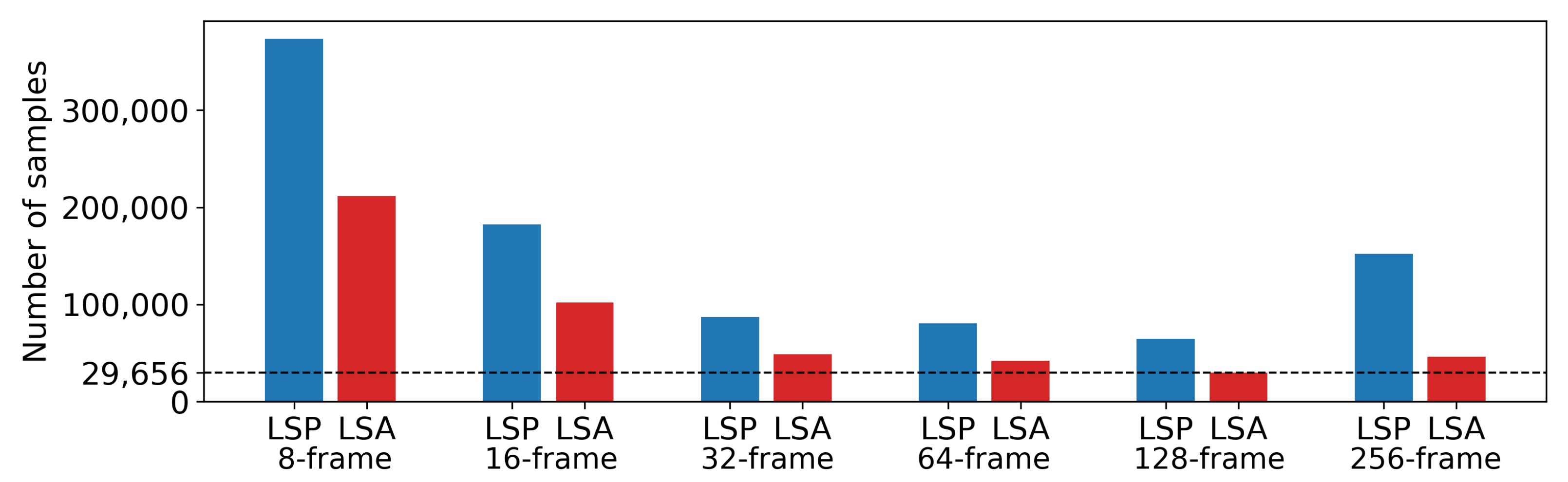
From the frames, we generated six datasets. The overview of the class distributions and the numbers of samples in each dataset is in Figure 1. All datasets contain M-mode images created by post-processing from B-mode. M-mode images are 2D depth/time slices of B-mode images through lung tissue. Sample counts of the M-mode datasets range from 94,454 to 284,342, with a class ratio of lung sliding absence to lung sliding presence ranging from 1:1.8 to 1:3.3. The process of generating these samples has two hyperparameters. The first, step parameter, represents the number of frames between two batches of M-mode images. The step parameter is set to 8 and 16 for 8- and 16-frame datasets, to 32 frames for 32-, 64-, and 128-frame datasets and again to 16 frames for the 256-frame dataset. The second parameter is the selection range, representing the range of x-coordinates in B-mode images. The value of the selection range is dynamically selected for each image based on the extent of lung tissue in the current image that conveys information about lung sliding.

Segmentation Labels

The LUS video files must be labelled by a highly trained expert, but the procedure is not time-consuming. On the other hand, labelling a 2D dataset for basic semantic segmentation in LUS takes more time but requires only a low level of expertise. We educated a group of 80 volunteers, who drew rectangular bounding boxes around the objects of interest using a labelImg tool [15]. Labelling was the first step in the production of semantic segmentation masks.

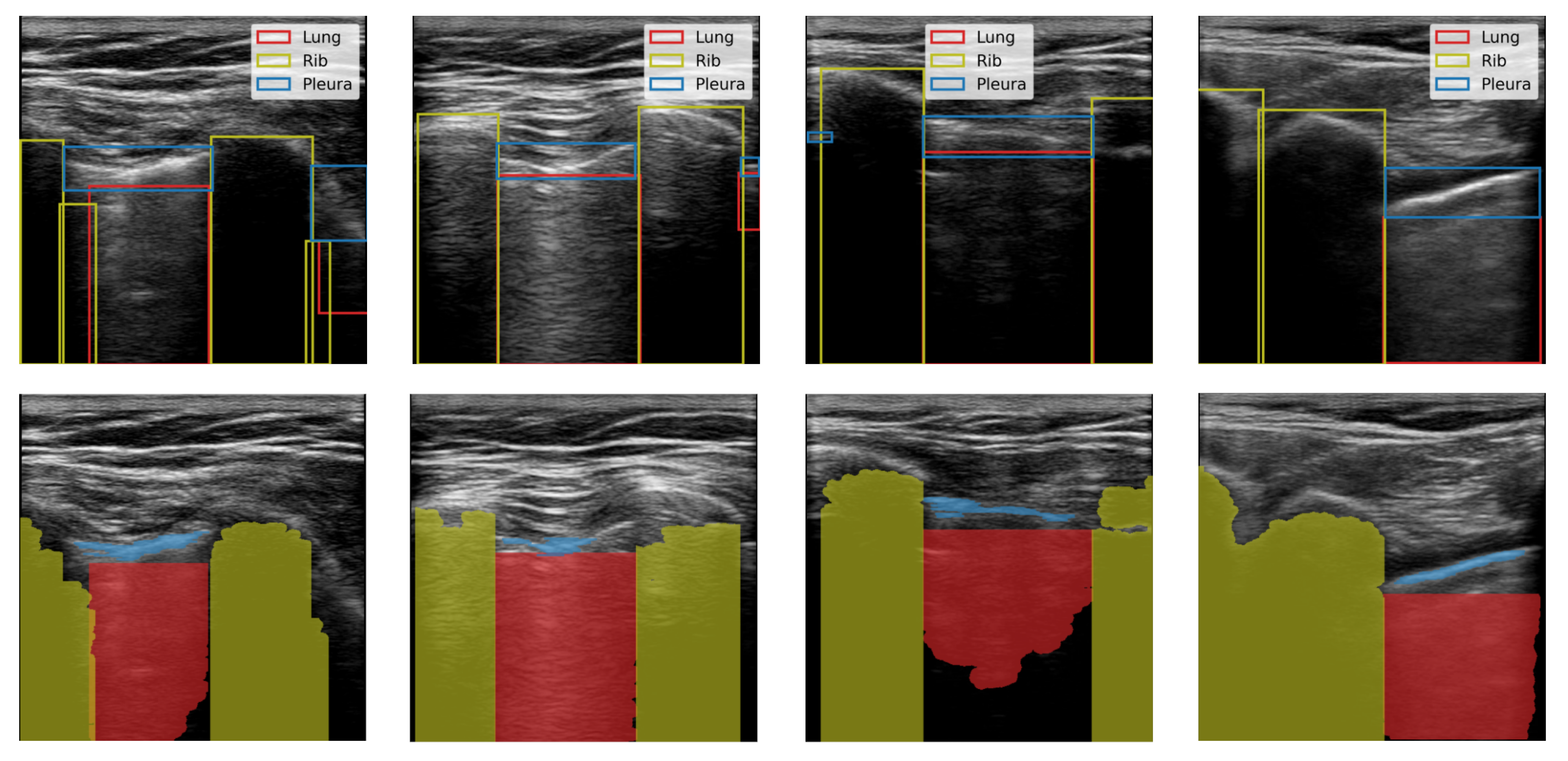
We randomly selected 6400 frames from 545 videos, and each volunteer labelled 80 frames. The objects of interest were the pleura, lung, rib, and tissue. Class pleura represents both the parietal and visceral pleura. In the LUS images, it is a shimmering white line connecting the lung and chest wall. Class lung is the area under the pleura between the anechoic shadows of the ribs. Class ribs represents the area of anechoic shadow. This artifact appears because sound waves are reflected well by the hard material of the ribs. Finally, the class tissue represents the chest wall, consisting of skin, fat, and muscle tissue.

We produced binary semantic segmentation masks for the objects of interest by applying several computer vision algorithms to the areas delimited by the bounding boxes, see Figure 2. We assumed that the objects of interest differed from other objects in the bounding box by brightness. To create the segmentation mask for the lung class, we applied intensity thresholding in the bounding box with a threshold value determined by Otsu’s method. The initial result was refined by morphological dilation, and the holes in the mask were filled. Finally, the mask was returned to the coordinate system of the image. We repeated this process for each bounding box in an image. In the end, we kept only the largest contiguous region because some of the images contained multiple separate regions of the lung. We generated pleura masks using the same process. Similarly, masks were created for the rib class however, we inverted the mask produced by Otsu’s method and kept two separate regions.

2.2. Automated M-Mode Classification

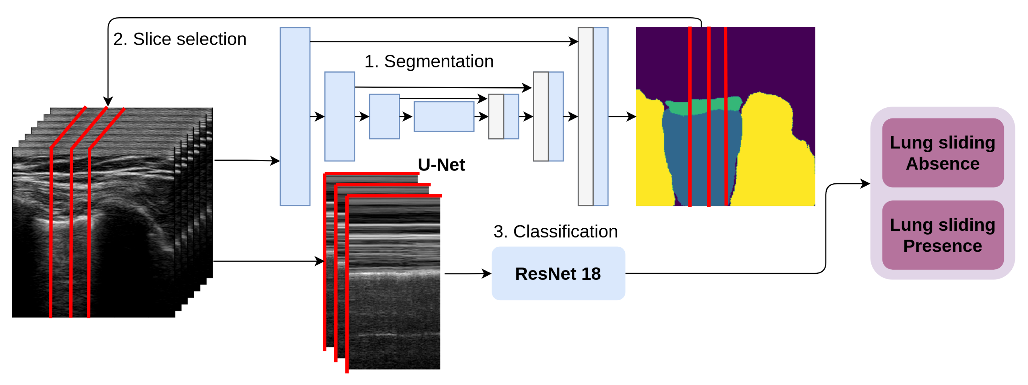
Automated M-mode classification (see Figure 3) classifies lung sliding motion with a 2D CNN on a 2D data slice selected across the temporal resolution of the video. Physicians use the M-mode view of the data to confirm their qualitative estimate about lung sliding. This method automates two tasks performed by a physician: Slice selection and estimation of the presence of lung sliding presence. First, our architecture takes the first frame from the series, and the U-Net predicts the segmentation mask for the selected tissues of interest; second, it uses the tissue masks to select the x-coordinate of a one pixel-wide column selected in the sequence of frames to form 2D temporal slices. These slices represent the CNN’s input, and they are sorted into two categories: LSP and LSA.

2.2.1. Semantic Segmentation of Lung Ultrasound

For the segmentation of the lung, pleura, and rib, we used the fully convolutional architecture U-Net [16], Figure 3. Our model contains three encoder and three decoder blocks. Each block uses a 2D convolutional layer, 2D batch normalisation, and a rectified linear unit layer, in that order, twice, followed by either 2D max-pooling in the case of the encoder block or 2D transposed convolution in the case of the decoder block. The first two encoder blocks connect to a deeper layer and skip-connect to the corresponding decoder layer with the same resolution. The third and deepest encoder block connects directly to the deepest decoder block. Decoder blocks take the skip-connected output from the encoder block and the output from the decoder’s deeper layer and produce the input for the higher-resolution decoder block. Finally, the prediction is made using a softmax layer. Loss is calculated as weighted pixel-wise cross-entropy. The weight is determined as a class distribution from a random subsample of the dataset. In the pleura segmentation, decreasing the weight of pleura segments by 80% improved the segmentation results.

The input image resolution is $480\times 480$ pixels. We used four types of data augmentation: Vertical and horizontal flipping, random rotation, translation, and scaling. We trained the neural networks for 30 epochs with early stopping that occurred when, after 10 epochs, the validation loss did not drop below the lowest previously recorded value. We randomly divided the dataset into three parts: 50% for training and 25% each for validation and testing.

To improve the resulting segmentation, we applied post-processing for the pleura, lung, and rib:

• The connected regions in the prediction mask are detected;
• The largest connected region is kept, and the rest are discarded. In the case of the rib class, the two largest connected regions are kept;
• The holes in the largest connected region are filled.

2.2.2. Slice Selection

In M-mode images, we distinguish two patterns: Seashore and barcode. Seashore patterns exhibit a noise-like appearance, which comes mainly from the lung tissue artifact. In order to capture these patterns, M-mode slices must at least partially intersect the lung tissue artifact. Therefore, we propose two methods for slice selection in the automated M-mode classification:

• Lung slice selection: We use our U-Net to segment the lung tissue. All the slices between the minimum and maximum of the lung mask x-coordinate are passed to the classification network. This approach ensures that all the slices that contain information about lung sliding are forwarded for classification.
• Centroid slice selection: We use binary segmentation U-Nets for three tissues, lung, pleura, and rib. We use the centroid of the lung and pleura to select two slices. To select the final slice, we use the rib mask. First, we ascertain whether we have one or two rib tissue segments. Then, if we have two segments, we use the mean of the x-coordinates of both centroids; otherwise, we replace one, either 0 or image width, based on the position of the other rib segment.

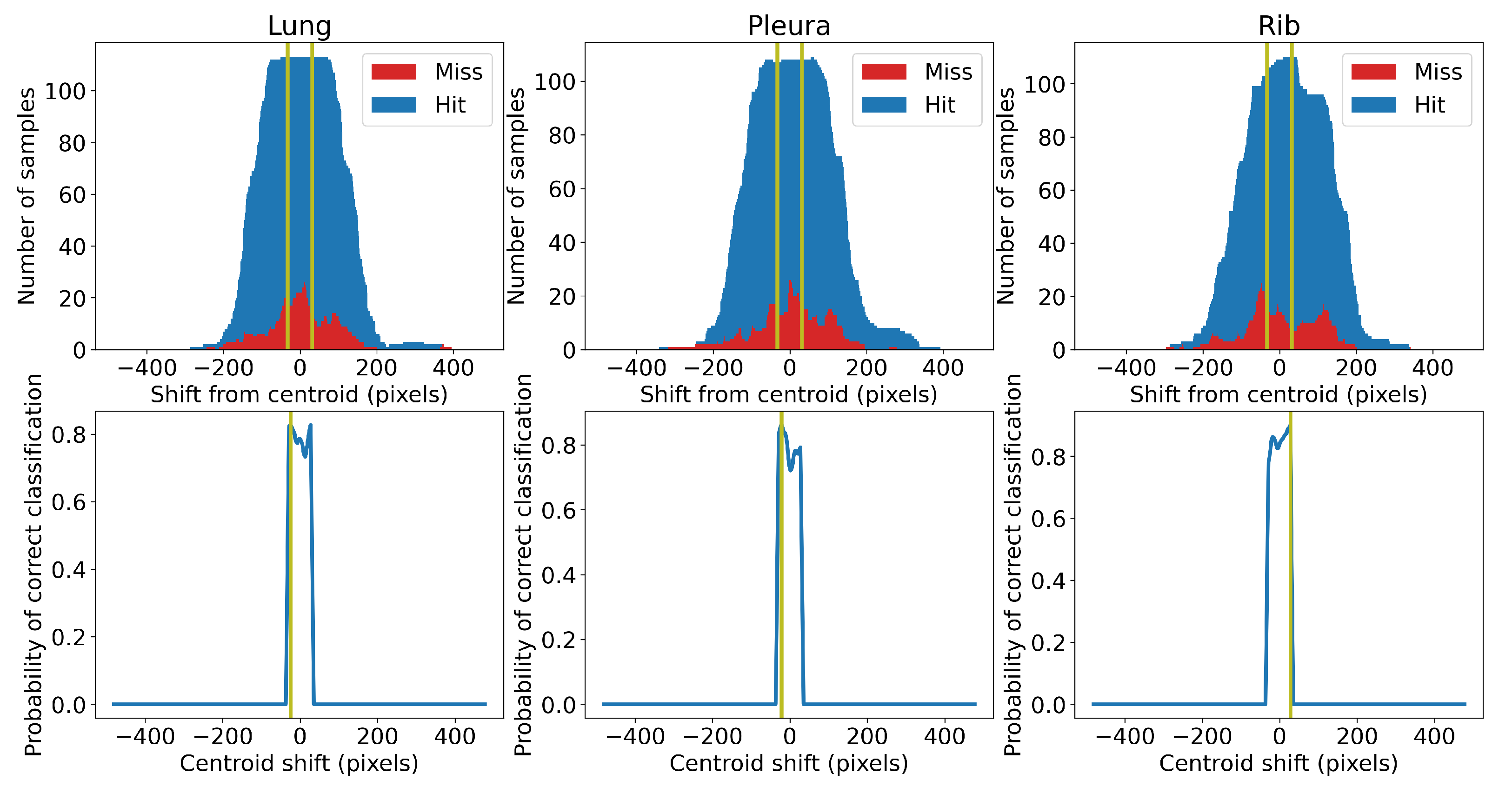
Centroid selection is a sub-optimal method to select M-mode slices, since the x-coordinate of the centroid is not always the optimal slice, i.e., it is not an x-coordinate giving the highest probability of correct classification. Moreover, it inherits bias from the segmentation networks. The optimal position of the slice may be shifted left or right from the centroid. We used a statistical approach to find the optimal shift value. First, we trained five different classifiers to categorise the lung slice selection. We then classified slices randomly taken from the training samples while keeping track of the position of the slices relative to the estimated centroid. We calculated the counts of the correctly and incorrectly classified slices and plotted them against the distance of the slices from the estimated tissue centroid (positive distance is to the right, negative to the left; see Figure 4). The optimal shift from a specific centroid is the value giving the highest probability of correct classification of the slice. We limited the shift to be within the range of $\pm K$ pixels from the centroid. In our case, we set this hyperparameter to 32 pixels. We added these constant shifts to calculated positions of the centroids. The values we found were $-10$, $-19$ and +28 pixels for the centroids calculated for the lung, pleura, and rib tissue, respectively.

2.2.3. M-Mode Classification

The M-mode image is a 2D slice across the temporal dimension in the ultrasound video, as shown in Figure 3. For the classification of this type of image, we used ResNet 18 [17]. Input dimensions were $3\times H\times N$, where H is the image height, N is the number of frames, and the number 3 is the number of channels. The greyscale input images were stacked three times to simulate three-channel RGB images. The model is 18 layers deep. First, the input is passed to the convolutional layer, batch normalisation, and ReLU activation, followed by the max-pooling layer. Second, these features were forwarded to a series of residual blocks. Features from the last residual block were flattened by adaptive average pooling. Average pooling features were fully connected to the network output. Finally, the binary prediction was made using a softmax layer. The loss was calculated as a weighted cross-entropy, where the weights represent the class distribution.

All the presented models were pre-trained on the ImageNet database and then fine-tuned for a maximum of 15 epochs, with early stopping when the validation loss did not improve in five consecutive epochs. We used the Adam optimisation algorithm with the learning rate set to 0.001. The dataset was split into four stratified folds with patient-wise split. We always used three out of four folds for the training and validation of the neural network. The training and validation datasets follow the patient-wise split, and the ratio between them is 1.5:1. To ensure validity of our methodology, we present the results from the fourth fold, which was not used in training or validation.

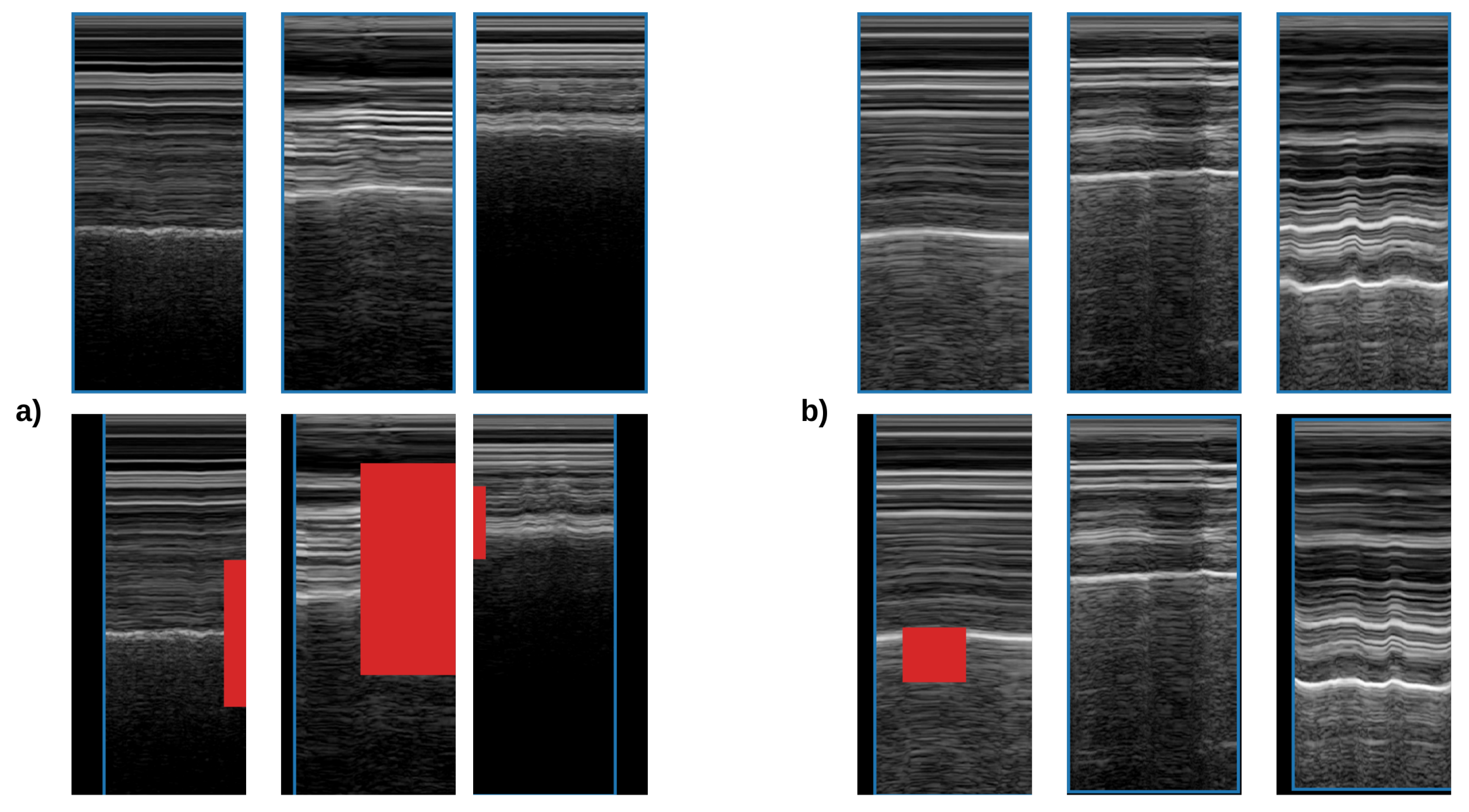
For data augmentation, we used random erasing [18] and random affine transformations (rotation, translation, and scaling), see Figure 5. The probability of the transforms was set equally to $0.5$. Rotation ranged between $[-10,10]$ degrees and horizontal translation between $[-0.1,0.1]$ of the image height; vertical translation ranged between $[-0.1,0.1]$ of the image width, and size scales ranged from $0.9$ to $1.1$ of the original size. Random erasing removed rectangular areas (pixels values set to 0) between $[0.05,0.33]$ of the image area.

2.3. Evaluation and Aggregation

We trained separate models for binary segmentation of the individual tissues (lung, pleura, and rib). Therefore, the accuracy represents the ratio of the correctly classified pixels to all pixels in the mask. Precision measures the proportion of the correctly classified tissue pixels to all pixels classified as the tissue. Recall measures the proportion of the correctly classified background pixels to all pixels classified as the background. IoU measures the overlap between the correctly identified tissue pixels and the area of the union of all pixels identified as tissue pixels and misclassified background pixels.

In the classification task, lung sliding absence is our target class. Accuracy represents the ratio of correctly classified samples with lung sliding presence and lung sliding absence to all samples. Balanced accuracy is the average accuracy per class to counteract the class imbalance. Sensitivity measures the proportion of correctly classified samples with the absence of lung sliding to all samples thus classified; specificity measuring the proportion of correctly classified samples with the presence of lung sliding to all samples thus classified.

Lung sliding is a time-structured process. In our classification system, to obtain the final prediction of whether lung sliding is present for either a sequence of frames (volume) or the whole video file, we take into account several predictions. We use two types of prediction aggregation in our classification system: Volume and video aggregation. In both cases, we apply averaging. Volume aggregation represents the aggregation of samples from a single sequence of frames with dimensions $H\times W\times N$; video aggregation is an aggregation of the volume predictions for the whole video. Let ${\widehat{y}}_t$ be the binary prediction of the classifier for a sequence of frames (a sample) starting at time t. We aggregate this prediction by averaging as follows:

$$y_{agg}\left({\widehat{y}}_t\right)=\frac{1}{N_{samples}}\sum _{t=0}^{N_{samples}-1}{\widehat{y}}_t$$

(1)

where $N_{samples}$ is the number of samples from the specific video file. The volume aggregation is performed correspondingly. Let $y_t$ be the ground truth for the binary classification for the sample starting at time t; then the aggregated video accuracy is:

$$ac{c}_{video}({\widehat{y}}_t,y_t)=\frac{1}{N_{samples}}\sum _{t=0}^{N_{samples}-1}{\widehat{y}}_t=y_t$$

(2)

where $N_{samples}$ is the number of samples from the specific video file. This measure is the ratio of correctly classified samples from the video file to all samples from the given video. To measure the performance of a classifier on a set of testing videos, we introduce thresholded aggregated accuracy $ta{a}_{threshold}$, which represents the ratio of the number of video files with the aggregated video accuracy over the given threshold to the number of all files. For example, $ta{a}_{75}$ is defined as follows:

$$ta{a}_{75}=\frac{1}{N_{videos}}\sum _{t=0}^{N_{videos}-1}ac{c}_{video}({\widehat{y}}_t,y_t)>0.75$$

(3)

where $N_{videos}$ is the total number of video files. $ta{a}_{75}$ represents the ratio of video files that have, in aggregate, more than 75% of samples correctly classified.

3. Experimental Results

This section is divided into two subsections: We first report the semantic segmentation results and then the automated M-mode classification results. In the M-mode classification results, we experiment with the number of input frames for the classification and slice selection method. The number of frames represents the size of the sliding window selecting an input through video, and the slice selection method represents one of two methods for selecting a slice in a current sample; see Section 2.2.2. We performed hypothesis testing for significant differences at the 5% significance level.

3.1. Segmentation Results

Table 1. Average performance of U-Net in binary segmentation of the lung, pleura, and rib. (Ratio: Target class:background; Acc.: Accuracy; IoU: Intersection over union.)

Tissue	Ratio	Accuracy	Precision	Recall	IoU
Lung	1:4.6	0.93	0.94	0.79	0.75
Pleura	1:36.2	0.98	0.75	0.71	0.61
Rib	1:4.4	0.90	0.93	0.72	0.81

shows the average of performance metrics a ten-times-repeated hold-out validation of U-Nets’ binary segmentation of the pleura and the lung for the test dataset. Post-processing was applied according to Section 2.2.1. We used accuracy, precision, recall, and IoU to evaluate each segmentation network.

All of the segmentation networks achieved an accuracy above 90%. Precision of the segmentation for the classes lung and rib is above 93%. Segmentation of pleura, which has a class:background ratio of 1:36.2, achieves a precision of 75%. Recall of all classifiers is between 71% and 79%. The IoU is 75%, 61%, and 81% for the lung, pleura, and rib, respectively.

3.2. Automated M-Mode Classification Results

Table 2. Average M-mode image classification performance metrics with standard deviations of ResNet18 with different numbers of input frames. (N: Number of frames; Slice sel.: Slice selection method according to Section 2.2.2; Bal. Accuracy: Balanced accuracy.)

N	Bal. Accuracy	Sensitivity	Specificity
8	0.71 ± 0.07	0.65 ± 0.17	0.76 ± 0.16
16	0.76 ± 0.08	0.76 ± 0.14	0.75 ± 0.16
32	0.77 ± 0.08	0.77 ± 0.15	0.77 ± 0.17
64	0.78 ± 0.07	0.78 ± 0.14	0.78 ± 0.14
128	0.74 ± 0.11	0.65 ± 0.21	0.83 ± 0.14
256	0.62 ± 0.15	0.44 ± 0.35	0.81 ± 0.23

shows an average sample classification performance over a ten-times-repeated fourfold stratified cross-validation with patient-wise split. We present six ResNets with varying input size. The number of frames ranges from 8 to 256. Therefore, the smallest input size is $3\times 480\times 8$ and the largest is $3\times 480\times 256$. Balanced accuracy ranges from 62% to 78%, with the best-performing model at 64 frames and the worst-performing model at 256 frames; 64-frame and 256-frame models are also the best- and the worst-performing, respectively, in sensitivity. On the other hand, the most specific model is the 128-frame version, with 83% specificity and 65% sensitivity.

The video aggregation results presented in

Table 3. Average video classification performance metrics of automated M-mode classification with different numbers of input frames and different slice selection methods. (NoF: Number of frames; Slice sel.: Slice selection method according to Section 2.2.2; Bal. Accuracy: Balanced accuracy; $ta{a}_{75}$: Thresholded aggregated accuracy according to Section 2.3; Sens.: Sensitivity; Spec.: Specificity; P-pair: p-value of the paired two-sided permutation test for slice selection method; P-frame: p-value of two-sided permutation test against the best classifier.)

NoF	Slice Sel.	Bal. Acc.	${\mathbf{taa}}_{75}$	Sens.	Spec.	P-Pair	P-Frame
8	lung	0.78	0.57	0.70	0.86	0.049	0
	centroid	0.75	0.60	0.64	0.86
16	lung	0.88	0.63	0.88	0.88	0.290	0.168
	centroid	0.86	0.68	0.83	0.90
32	lung	0.89	0.70	0.87	0.91	0.085	0.223
	centroid	0.86	0.72	0.82	0.91
64	lung	0.91	0.71	0.89	0.93	0.210	-
	centroid	0.89	0.75	0.86	0.92
128	lung	0.81	0.69	0.69	0.94	0.600	0.003
	centroid	0.81	0.74	0.66	0.95
256	lung	0.68	0.65	0.47	0.88	0.222	0
	centroid	0.70	0.68	0.52	0.87

are an average of ten-times-repeated fourfold stratified cross-validation with patient-wise split. Six ResNets were trained with varying numbers of input frames; their sample classification performance is available in Table 2. Two types of averaging aggregation are performed: Volume and video aggregation. Volume aggregation is either performed within all slices of a lung or within three slices in a single volume; see Section 2.2.2 for details. Video aggregation puts these predictions together with a fixed step of eight frames for the whole duration of the video sample. The step size is the minimal number of frames (N = 8) to minimise the information loss during aggregation.

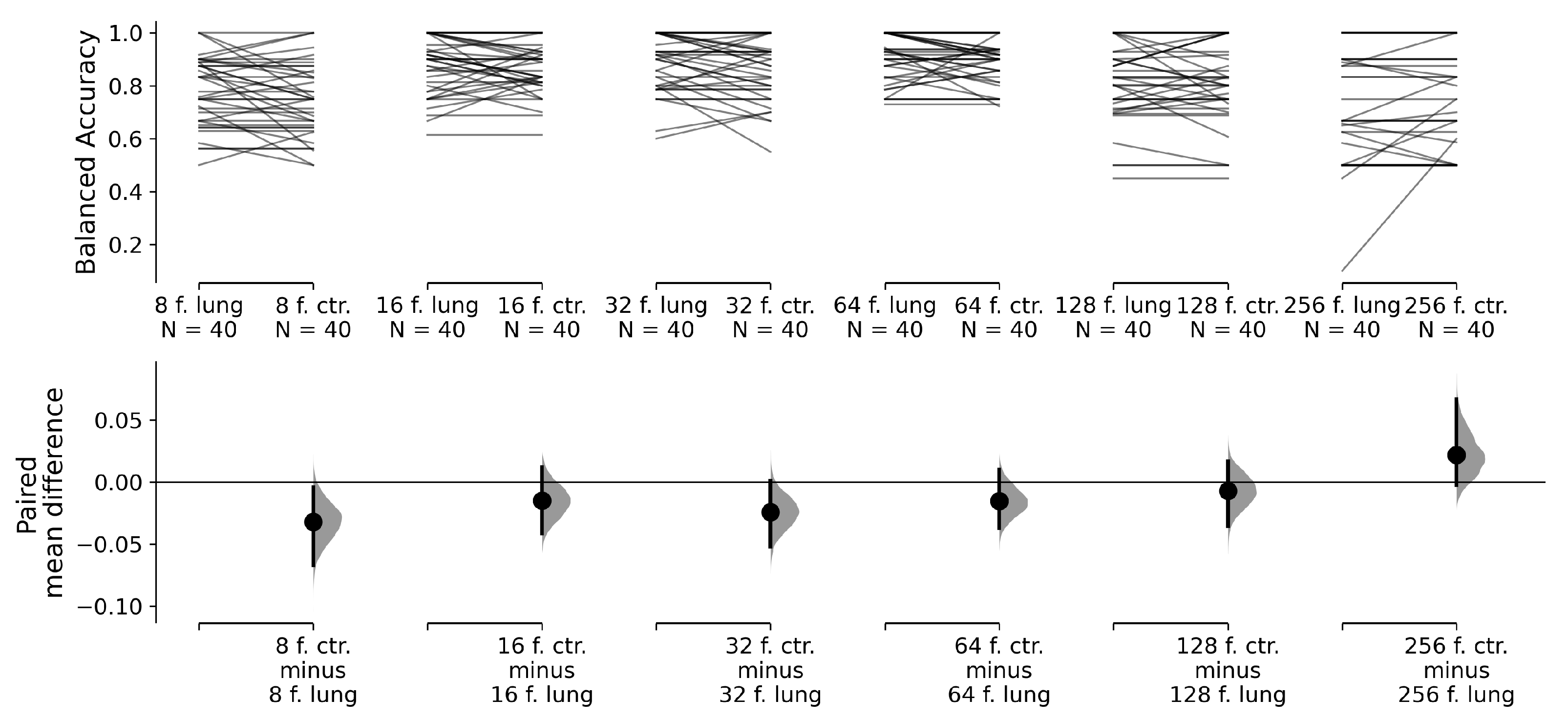
This approach produces pairs of classifiers that only differ in terms of the selection of the input slices from the input volume. With this test design, we can perform paired tests between an 8-frame ResNet 18 with lung slice selection and the same 8-frame ResNet 18 with centroid slice selection; between a 16-frame ResNet 18 with lung slice selection and a 16-frame ResNet 18 with centroid slice selection; and so on. Our null hypothesis is that the balanced accuracy means between the pairs of classifiers are equal. The alternative hypothesis is that the balanced accuracy means are not equal. We use estimation statistics to compare the mean differences between our classifier pairs [19]. The reported p-values of the two-sided permutation t-test are the likelihoods of observing the effect sizes if the null hypothesis (zero difference in balanced accuracy) is true. For each p-value, 5000 reshuffles of the lung slices selection and centroid slice selection classifier accuracies were performed.

Visualisation of the paired permutation t-tests is in Figure 6. While there is difference in a balanced accuracy mean between 8-frame classifiers for lung slice selection and centroid slice selection at 5% significance level, 16-to-256-frame classifiers for lung slice selection and centroid slice selection pairs do not exhibit differences in the balanced accuracy mean at the 5% significance level. Therefore, for our final hypothesis testing, we preferred classifiers with centroid slice selection, which require only three slices per volume to make volume aggregation, when the differences between classifiers were statistically insignificant. If there was a significant difference between lung and centroid slice selection, we preferred the classification method with a higher balanced accuracy. In Table 3, in row slice selection, we highlight the chosen slice selection method.

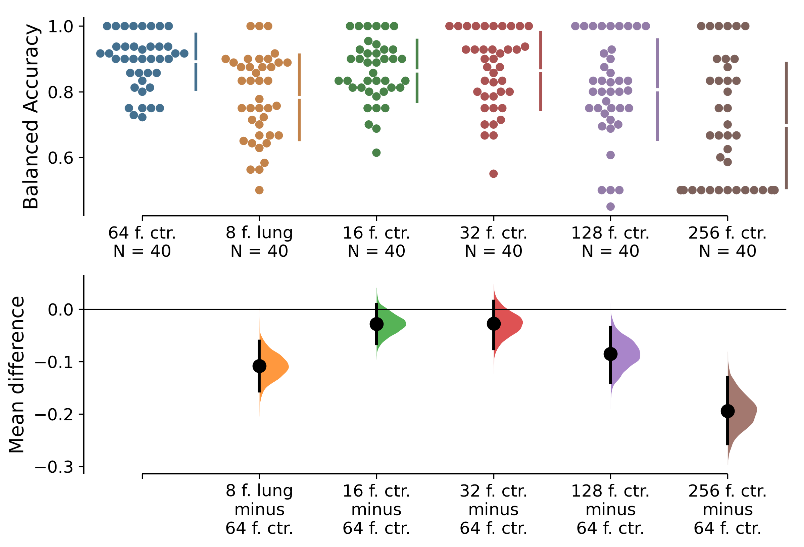
Visualisation of permutation t-tests between the best performing 64-frame classifier and other classifiers with different numbers of input frames and chosen slice selection methods can be found in Figure 7. The null hypothesis is that the balanced accuracy means between the best classifier and the rest of the classifiers are equal. The alternative hypothesis is that the balanced accuracy means are not equal. We observe that the balanced accuracy means are significantly worse for the 8-, 128-, and 256-frame classifiers than for the 64-frame one. There is no significant difference between the 16- and 32-frame classifiers and the best-performing 64-frame classifier. Furthermore, we highlight the performance of three classifiers on metric $ta{a}_{75}$ in 32-, 64-, and 128-frame versions that achieve $ta{a}_{75}$ above 70% with at least one of the slice selection methods.

4. Discussion

Our architecture selects temporal slices for the detection of lung sliding based on tissue segments of the lung, pleura, and ribs. The U-Net for lung and rib segmentation outperforms the U-Net for pleura segmentation by almost every measure; see Table 1. These performance differences result from different tissue-to-background ratios and possible mislabelling during the process of semi-automated production of semantic segmentation masks. The lung tissue and rib shadows are well constrained. The lung tissue is constrained by the pleura and the anechoic shadows of the ribs, but the contours of the pleura tissue are fuzzier.

We compare two types of slice selection: Lung slice selection and centroid slice selection. While lung slice selection uses different sample amounts for each volume, centroid slice selection extracts three slices per volume. Only the 8-frame classifier performs significantly worse with centroid slice selection; see Figure 6. However, our best-performing classifiers—the 16-, 32-, and 64-frame versions—do not display significant differences between the two slice selection methods.

Lung sliding is a dynamic phenomenon. We must take into account the frame rate of the video and physiology of the process that we are trying to detect. Videos from our dataset contain 30 frames per second. In our case, the best-performing classifiers were the ones for 16-, 32-, and 64-frame input time windows, that is, periods of 0.53–2.13 s. Therefore, for detection of the absence of lung sliding, we recommend using time windows between 0.53 and 2.13 s.

The dataset used in this study consists of LUS samples taken with a single device from patients after thoracic surgery in a single institution. While we do not think that this invalidates the presented research results, the dataset is affected by this bias. It is reasonable to assume that the classifiers would perform slightly differently if the samples were taken with several US devices of varying imaging quality.

5. Conclusions and Future Research

CNNs are suitable for lung sliding detection from clinical LUS videos. Our architecture, automated M-mode classification, achieved a balanced accuracy of 86–89% with its 16–64-frame versions. There were no significant differences in classification performance between the proposed lung and centroid slice selection methods in the best-performing classifiers. M-mode images are 2D temporal slices that form seashore or barcode patterns. These patterns are a key feature for the classification of M-mode images. In our opinion, physicians’ familiarity with these patterns and their simplicity marks the direction for future application in clinical practice. Furthermore, automatic selection of the M-mode slice simplifies the detection of the absence of lung sliding and relieves a physician from having to perform manual slice selection.

Our methods utilise black-box classifiers, CNNs, that implicitly do not provide any explanation. As a part of future research, we plan to visualise the input data by highlighting the areas that contribute the most to the CNN’s decisions and by creating a more elaborate decision support system. Furthermore, explainability methods for CNNs such as [20,21,22] could provide valuable insight to reinforce or contradict the physician’s decision. Following the application of 2D CNNs for lung sliding absence detection from M-mode images, we want to detect lung sliding directly from B-mode images with 3D CNNs. We plan to expand the dataset size to make it more applicable to the training of 3D CNNs. Furthermore, our dataset currently contains only two classes: Presence and absence of lung sliding. The absence of lung sliding patterns does not, by itself, provide sufficient information for pneumothorax detection. Therefore, the next logical step is the detection of lung point, which confirms pneumothorax. In addition, the detection and localisation of A-line and B-line artifacts may provide more insight into the correlation between lung sliding motion, the position of lung point, and these artifacts.

References

- Smargiassi, A.; Inchingolo, R.; Chiappetta, M.; Ciavarella, L.P.; Lopatriello, S.; Corbo, G.M.; Margaritora, S.; Richeldi, L. Agreement between chest ultrasonography and chest X-ray in patients who have undergone thoracic surgery: Preliminary results. Multidiscip. Respir. Med. 2019, 14, 1–7. [Google Scholar] [CrossRef]
- Malík, M.; Dzian, A.; Skaličanová, M.; Hamada, L.; Zeleňák, K.; Grendár, M. Chest ultrasound can reduce the use of X-ray in postoperative care after thoracic surgery. Ann. Thorac. Surg. 2020. [Google Scholar] [CrossRef] [PubMed]
- Kim, K.; Choi, H. High-efficiency high-voltage class F amplifier for high-frequency wireless ultrasound systems. PLoS ONE 2021, 16, e0249034. [Google Scholar]
- Mayo, P.; Copetti, R.; Feller-Kopman, D.; Mathis, G.; Maury, E.; Mongodi, S.; Mojoli, F.; Volpicelli, G.; Zanobetti, M. Thoracic ultrasonography: A narrative review. Intensive Care Med. 2019, 1–12. [Google Scholar] [CrossRef] [PubMed]
- Lichtenstein, D.A.; Meziere, G.A. Relevance of lung ultrasound in the diagnosis of acute respiratory failure*: The BLUE protocol. Chest 2008, 134, 117–125. [Google Scholar] [CrossRef] [PubMed] [Green Version]
- Lichtenstein, D.A.; Menu, Y. A bedside ultrasound sign ruling out pneumothorax in the critically III: Lung sliding. Chest 1995, 108, 1345–1348. [Google Scholar] [CrossRef] [PubMed] [Green Version]
- Heidecker, J.; Huggins, J.T.; Sahn, S.A.; Doelken, P. Pathophysiology of pneumothorax following ultrasound-guided thoracentesis. Chest 2006, 130, 1173–1184. [Google Scholar] [CrossRef]
- Husain, L.F.; Hagopian, L.; Wayman, D.; Baker, W.E.; Carmody, K.A. Sonographic diagnosis of pneumothorax. J. Emerg. Trauma Shock 2012, 5, 76. [Google Scholar] [CrossRef] [PubMed]
- Lichtenstein, D.A. BLUE-protocol and FALLS-protocol: Two applications of lung ultrasound in the critically ill. Chest 2015, 147, 1659–1670. [Google Scholar] [CrossRef] [PubMed] [Green Version]
- Summers, S.M.; Chin, E.J.; April, M.D.; Grisell, R.D.; Lospinoso, J.A.; Kheirabadi, B.S.; Salinas, J.; Blackbourne, L.H. Diagnostic accuracy of a novel software technology for detecting pneumothorax in a porcine model. Am. J. Emerg. Med. 2017, 35, 1285–1290. [Google Scholar] [CrossRef] [PubMed]
- Lindsey, T.; Lee, R.; Grisell, R.; Vega, S.; Veazey, S. Automated Pneumothorax Diagnosis Using Deep Neural Networks. In Progress in Pattern Recognition, Image Analysis, Computer Vision, and Applications; Springer International Publishing: Cham, Switzerland; Madrid, Spain, 2019; pp. 723–731. [Google Scholar] [CrossRef] [Green Version]
- Kulhare, S.; Zheng, X.; Mehanian, C.; Gregory, C.; Zhu, M.; Gregory, K.; Xie, H.; Jones, J.M.; Wilson, B. Ultrasound-based detection of lung abnormalities using single shot detection convolutional neural networks. In Simulation, Image Processing, and Ultrasound Systems for Assisted Diagnosis and Navigation; Springer: Berlin/Heidelberg, Germany, 2018; pp. 65–73. [Google Scholar] [CrossRef]
- Ren, S.; He, K.; Girshick, R.; Sun, J. Faster R-CNN: Towards real-time object detection with region proposal networks. IEEE Trans. Pattern Anal. Mach. Intell 2016, 39, 1137–1149. [Google Scholar] [CrossRef] [PubMed] [Green Version]
- Mehanian, C.; Kulhare, S.; Millin, R.; Zheng, X.; Gregory, C.; Zhu, M.; Xie, H.; Jones, J.; Lazar, J.; Halse, A.; et al. Deep learning-based pneumothorax detection in ultrasound videos. In Smart Ultrasound Imaging and Perinatal, Preterm and Paediatric Image Analysis; Springer: Berlin/Heidelberg, Germany, 2019; pp. 74–82. [Google Scholar] [CrossRef]
- Tzutalin, D. Labelimg. Available online: https://github.com/tzutalin/labelImg (accessed on 14 June 2021).
- Ronneberger, O.; Fischer, P.; Brox, T. U-net: Convolutional networks for biomedical image segmentation. In Proceedings of the International Conference on Medical Image Computing and Computer-Assisted Intervention, Munich, Germany, 5–9 October 2015; Springer: Berlin/Heidelberg, Germany, 2015; pp. 234–241. [Google Scholar] [CrossRef] [Green Version]
- He, K.; Zhang, X.; Ren, S.; Sun, J. Deep residual learning for image recognition. In Proceedings of the IEEE Conference on Computer Vision and Pattern Recognition, Las Vegas, NV, USA, 27–30 June 2016; pp. 770–778. [Google Scholar]
- Zhong, Z.; Zheng, L.; Kang, G.; Li, S.; Yang, Y. Random Erasing Data Augmentation. In Proceedings of the AAAI Conference on Artificial Intelligence, New York, NY, USA, 7–12 February 2020; pp. 13001–13008. [Google Scholar] [CrossRef]
- Ho, J.; Tumkaya, T.; Aryal, S.; Choi, H.; Claridge-Chang, A. Moving beyond P values: Data analysis with estimation graphics. Nat. Methods 2019, 16, 565–566. [Google Scholar] [CrossRef] [PubMed]
- Shrikumar, A.; Greenside, P.; Kundaje, A. Learning important features through propagating activation differences. In Proceedings of the International Conference on Machine Learning, Sydney, Australia, 6–11 August 2017; pp. 3145–3153. [Google Scholar]
- Selvaraju, R.R.; Cogswell, M.; Das, A.; Vedantam, R.; Parikh, D.; Batra, D. Grad-cam: Visual explanations from deep networks via gradient-based localization. In Proceedings of the IEEE International Conference on Computer Vision, Venice, Italy, 22–29 October 2017; pp. 618–626. [Google Scholar] [CrossRef] [Green Version]
- Sundararajan, M.; Taly, A.; Yan, Q. Axiomatic attribution for deep networks. In Proceedings of the International Conference on Machine Learning, Sydney, Australia, 6–11 August 2017; pp. 3319–3328. [Google Scholar] [CrossRef]