Abstract
Lipreading aims to recognize sentences being spoken by a talking face. In recent years, the lipreading method has achieved a high level of accuracy on large datasets and made breakthrough progress. However, lipreading is still far from being solved, and existing methods tend to have high error rates on the wild data and have the defects of disappearing training gradient and slow convergence. To overcome these problems, we proposed an efficient end-to-end sentence-level lipreading model, using an encoder based on a 3D convolutional network, ResNet50, Temporal Convolutional Network (TCN), and a CTC objective function as the decoder. More importantly, the proposed architecture incorporates TCN as a feature learner to decode feature. It can partly eliminate the defects of RNN (LSTM, GRU) gradient disappearance and insufficient performance, and this yields notable performance improvement as well as faster convergence. Experiments show that the training and convergence speed are 50% faster than the state-of-the-art method, and improved accuracy by 2.4% on the GRID dataset.
1. Introduction
Lipreading, also known as visual language recognition, refers to decoding the content of the spoken text based on the visual information of the speaker’s lip movement. It has a wide range of applications
values in speech recognition [1], public safety [2], intelligent human–computer interaction [3], visual synthesis, etc.
Traditionally, the lipreading method can follow two stages. First, it extracted features from the mouth region. Discrete Cosine Transform [4,5] was considered the most popular feature extractor, and then it was fed to the Hidden Markov Model (HMM) [1,6,7]. At the same time, there are some similar methods proposed: the difference is that the feature extractor is replaced with a deep autoencoder, and HMMS was replaced with Long-Short Term Memory (LSTM) [8,9].
Deep learning methods have achieved great success [10,11] in many
complex tasks based on traditional machine learning [12,13,14]. Convolutional Neural Networks (CNNs) show superior performance in image and video feature extraction compared to traditional methods. For example, Stafylakis et al. [15] present a deep learning architecture for lipreading and audiovisual word recognition. Petridis et al. [16] proposed an end-to-end visual speech recognition system based on
fully connected layers and LSTM networks. At this stage, there are two solutions for the lipreading architecture based on deep learning, which are divided into
Connectionist Temporal Classification(CTC) [17]-based speech recognition [18,19] technology, and the attention-based sequence-to-sequence (seq2seq) [20] neural network translation model.
Speech recognition [18,21]
technology-based on the CTC approach has made a great breakthrough. For the lipreading problem, Refs. [22,23,24] used Convolutional Neural Network (CNN) [25,26] as a feature extractor,
Recurrent Neural Network(RNN) [27,28] as the feature learner, and CTC [17] as the objective function, training an end-to-end sentence-level lipreading architecture.
Its architecture outperforms experienced human lipreaders on the GRID dataset [29].
However, these architectures have two main problems. On the one hand, a simple feature extractor is not competent for feature extraction of video data. On the other hand, the use of RNN will have the defects of vanishing or exploding gradients.
The attention-based sequence-to-sequence model was first used in the neural network translation model [20] to solve the problem that the input sequence and output sequence are not aligned in time. For the lipreading problem, Refs. [30,31] use the Attention-based seq2seq model to build a WAS
(Watch, Attend and Spell) architecture. Outstanding performance in LRW [32] and GRID [29] datasets shows a
Word Error Rate(WER) of 23.8% on the LRW [32] dataset. However, recent work [33,34] shows that the attention-based sequence-to-sequence model cannot correctly align with the output sequence for longer input sequences, so it is hard to converge during the entire training process.
However, recent results [35] show that the convolutional architecture performs better than recurrent networks on audio synthesis and machine translation tasks. Ref. [36] proposed a general TCN model and did a series of evaluation experiments for all serialization tasks. The results show that the TCN performs better than the
primary recurrent neural network(e.g., BLSTM, BGRU) in a broad range of sequence model tasks.
In this work, we propose a state-of-the-art model that improves the performance of lipreading and the speed of convergence. First, we discard the basic BGRU or BLSTM neural network layer and replace it with a
TCN [36]. Secondly, we propose a more efficient and complex feature extractor based on a 3D convolutional network and ResNet50 [37]. Its efficiency is greatly improved compared with
standard feature extractors. Finally, we use the CTC [17] objective function as a decoder to implement an end-to-end sentence-level lipreading architecture. It needs to be emphasized that the use of the TCN architecture has a core effect on the improvement of lipreading performance. Experiments show that the training and convergence speed is 50% faster than the state-of-the-art method, and improved accuracy by 2.4% on the GRID dataset. Figure 1 shows the general architecture of lipreading.
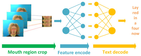
Figure 1.
The general end-to-end sentence-level lipreading architecture can be divided into three steps. (1) Cut out the regions of the mouth based on the alignment of the face in each frame of the video; (2) The feature extractor extracts visual features from the input image sequence. (3) A text encoder predicts the text output from the hidden feature matrix.
2. Related Works
Traditionally, for lipreading, Luettin et al. [38] first applied the
ASM model to lipreading, using a set of feature points to describe the inner or outer lip contour. This model has the disadvantage of manually labeling the training data. The quality of its feature extraction depends on the accuracy of the labeling, which requires more effort. The choice of the traditional lipreading system classifier depends on the task requirements. For large-scale continuous sentence recognition tasks, traditional methods generally use a decoding model based on GMM-HMM [8,39].
Research shows that recurrent networks (e.g., LSTM, GRU [28,40]) are more suitable for modeling sequence models than convolutional neural networks. Refs. [22,23,24,30] use CNN-RNN architecture, combining convolutional neural networks (CNNs) and recurrent networks (LSTM, GRU [28,40]) and training an end-to-end lipreading system. However, the recurrent network (RNN) has the defects of slow convergence, disappearing gradient, and local overfitting.
Deep learning practitioners commonly regard recurrent architectures as the default starting point for sequence modeling tasks. A well-regarded recent online course on “Sequence Models” focuses exclusively on recurrent architectures [41]. Recent studies [42,43,44] have shown that the convolutional architecture can achieve state-of-the-art performance accuracy in audio synthesis, word-level language modeling, and machine translation. This raises the question of whether these successes of convolutional sequence modeling are confined to specific application domains or whether a broader reconsideration of the association between sequence processing and recurrent networks is in order.
Recent studies [36] have shown that
TCN show superior performance compared to RNNs in most sequence modeling tasks, and overcome the shortcomings of RNNs, while demonstrating longer effective memory.TCN solves the defects of slow convergence, gradient explosion or disappearance, and local overfitting in RNN. In terms of lipreading, we should reconsider the common association between the lipreading architecture and the recurrent network, and regard TCN as the natural starting point for lipreading tasks.
3. Proposed Architecture
In this section, we introduce the proposed lipreading architecture. We should emphasize that the proposed architecture is an end-to-end sentence-level lipreading model. Figure 2 shows the implementation diagram of the architecture. Table 1 shows the implementation details of the architecture.
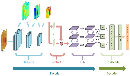
Figure 2.
The proposed architecture. A lipreading video containing N frames as input is followed by one layer of 3D-CNN, followed by a 3D average pooling layer. The 3D feature maps are passed through a residual network (ResNet50, [37]). The classification and fusion of feature maps are processed by the 2-layer TCN [36] network; and the TCN output of each time-step is processed by the linear layer and the softmax activation function. This end-to-end sentence-level lipreading architecture is trained using the CTC objective function.

Table 1.
The detailed of the proposed lipreading architecture.
3.1. 3D Convolutional Network
Convolutional Neural Networks (CNN) are commonly used to perform convolution operations on images to improve the performance of computer vision tasks, such as receiving image data as input [25]. The basic 2D convolutional layer mainly changes the channel C to C’ of the image. Figure 3a can clearly describe the process of 2D convolution. The convolution kernel of 3D convolution can be understood as a three-dimensional cube, as shown in Figure 3b.
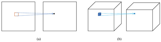
Figure 3.
Schematic diagram of convolution structure, (a) 2D convolution operation, (b) 3D convolution operation.
The 3D convolutional network is composed of 32 convolution kernels with a size of 3 × 3 × 3, followed by Batch Normalization (BN, [45]) and linear activation function (ReLU, [46]). Finally, the extracted feature map passes through the 3D average pooling layer, reducing the sampling rate and improving its robustness. The parameter weight of the 3D convolutional neural network is ∼16 K.
3.2. ResNet
At each time step, a 3D feature map is followed by a residual network (ResNet, [37]). Based on the needs of lipreading architecture design, we use the 50-layer ResNet version, which was proposed for ImageNet [47]. Its main innovation is residual learning, so that a deeper convolutional network can be trained. The most critical solution to achieve residual learning is short connections. What we need to emphasize is that we did not use its pre-trained weights on ImageNet [47], as they optimize completely different tasks and evaluate other protocols. The weight initialization we adopt is standard random initialization, and the random parameters obey Gaussian distribution.
3.3. Temporal Convolutional Network (TCN)
A recent study [36] has shown that a simple convolutional architecture is superior to classic recurrent convolutional networks, such as LSTM and GRU, on various tasks and datasets while exhibiting longer effective memory. Compared to the language modeling architecture of LSTM [28], TCNs have longer memory networks and can efficiently handle longer inputs.
We should emphasize that lipreading is the task of Sequence Modeling. Our goal is to replace BLSTM or BGRU with TCN to solve the a disappearing training gradient and slower convergence. Figure 4 shows the basic architecture of the TCN.
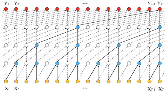
Figure 4.
The basic architecture of the Temporal Convolutional Network (TCN). (1) A sequence of feature maps () as input. (2) The feature maps are learned and decoded by Temporal Convolutional Network. (3) The TCN architecture finally produces a sequence of learning results ().
For the sequence modeling task, an input image sequence for , and we wish to predict some corresponding outputs at each time:
A simple causal convolution network can only have a limited size of feature information in the deep historical network. It is very challenging to build a sequence model using simple sequence convolution. Our solution is to implement a dilated convolution neural network to extend the receptive field. We use Dilated Convolutions to apply to the lipreading task and use Formula (2) to briefly describe its outline:
where as a 1D sequence input, as a filter, d is the dilation factor, k is the filter size, and accounts for the direction of the past.
More radically, we replace ordinary convolutional networks with a residual block [37]. It consists of a convolutional layer with 512-dimensional kernels of 5 size and the stride of 3 size, followed by Batch Normalization (BN, [45]), Rectified Linear Units (ReLU, [46]), and Dropout [48].
3.4. Connectionist Temporal Classification (CTC)
The CTC objective function [17] was originally widely used in speech recognition. In view of the similarity between speech recognition and lipreading, CTC was introduced in lipreading.
The core step of CTC is to convert the output of each time step of the sequence model into a probability distribution in the label sequences. The softmax activation function of the CTC network converts the output into a probability. The number of units is one more unit than the number of labels L; therefore, the output of each softmax layer can denote the probability distribution of the corresponding label.
Suppose a given input sequence of length T, followed by a Bi-LSTM recurrent neural network layer with m input, n output, and w weight. Therefore, define a continuous mapping to denote Bi-LSTM, : . Then, becomes the output of the sequence model(e.g., Bi-LSTM) and defines as the probability distribution of output k in time step t. We describe an alphabet . For each true label path, we obtain a probability by Formula (3):
Formula (3) is the product of the probability distribution under a path. There are many such paths from output to label. Given a mapping function from output to label , where is the combination of a series of possible labels. In the next step, we delete blank and duplicate labels in all paths (e.g., ). For any given label , through the inverse mapping of , we can obtain all of its paths. Calculate the probability sum of all paths by Formula (4):
Through the above Formula (4), we only need to obtain the most probable labeling of the input sequence as the output of CTC, as shown in Formula (5):
Finally, we use the CTC network to minimize Formula (6) as the training goal, and constantly update the weight parameters of the entire model:
In terms of lipreading, our dataset is video data and its corresponding text. Unfortunately, it is difficult to align video data and text in units. If we directly train the model without using alignment, it will be difficult for the model to converge due to the difference in people’s speech speed or the distance between characters. From the above description of CTC, we know that CTC is a solution that avoids manual alignment of input and output and is very suitable for lipreading or speech recognition applications. Therefore, CTC is a sensible choice for the lipreading task.
4. Database
This section describe the relevant dataset and evaluation protocol and perform evaluation on the dataset according to the relevant protocol.
4.1. GRID Dataset
For this study, we use the GRID dataset [29]. There are a total of 33,000 sentence sample videos, including 33 speakers. Each sentence consisted of a six-word sequence of the form indicated in Table 2. Of the six components, three—color, letter, and digit—were designated as “keywords”. Each sample video is fixed at 75 frames. The videos are recorded in a controlled lab environment, shown in Figure 5.
Table 2.
Sentence structure for the GRID dataset.
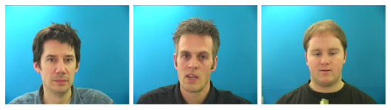
Figure 5.
Random frames from the GRID dataset.
4.2. Evaluation Protocol
We refer to the standard protocols in [22,49] to define an evaluation protocol. The Word Error Rate (short: ) is a way to measure the performance of lipreading. It compares a reference to an hypothesis and is defined like this:
where represent the number of substitutions, deletions, insertions, and words in the reference, respectively.
Character Error Rate () is another way to measure the performance of lipreading. It is very similar to Word Error Rate (). The difference is that words are replaced with characters.
5. Experiment
This section conduct experiments on the proposed architecture on a public benchmark dataset, summarize the corresponding performance data, and compare it with other state-of-the-art methods.
5.1. Data Alignment
The videos were processed with the DLib face detector, and the iBug face landmark predictor [50] with 68 landmarks coupled with an online Kalman Filter. Using these landmarks, we apply an affine transformation to extract a mouth-centered crop of size 112 × 112 × 3 pixels per frame. Therefore, each sample takes 75 × 112 × 112 × 3 data as the model input, where 75 is the number of frames of the video sample.
What we should emphasize is that the original data can not be used as the model input. Before, the data samples should be normalized to make the model more robust. In this experiment, we use Z-score normalization as the normalization process. The specific implementation process can be obtained from the following formula:
where is the final normalized result. Normalization processing is very critical for the model and can accelerate the convergence of the model.
5.2. Implementation Details
We use the proposed architecture for Tensorflow [51] training and testing. Table 1 summarizes the detailed parameters of the proposed architecture at each layer. The adopted back-propagation optimization algorithm is the ADAM optimizer [52], the initial learning rate is 0.0001, and the batch size is 8. Connectionist Temporal Classification (CTC) is used as the objective function. We trained the proposed architecture for 100 epochs on the public GRID dataset and reached a stable convergence point.
There are 33,000 sentence sample videos including 33 speakers on the GRID dataset [29]. This experiment randomly uses 31 speakers with 31,000 samples as the training set and two speakers with 2000 samples as the evaluation set. we should calculate the training loss, evaluation loss, the training and evaluation of Word Error Rate (WER), and Character Error Rate (CER) for every epoch.
For the GRID dataset, the proposed approach is compared with [22,23,24,30], which are referred to as ‘LipNet’, ‘WLAS’, ‘LCANet’, and ‘3D-2D-CNN-BLSTM’, respectively. In addition, in order to reflect the impact of key modules on the architecture, we separate the various modules of the architecture for comparison experiments.
5.3. Convergence Speed
What we should emphasize is that replacing the recurrent neural network (e.g., LSTM, GRU) with a Temporal Convolutional Network (TCN) [36] is for adequate training, speeding up the convergence speed, and preventing the disappearance of the gradient. We implemented a comparison of four different architectures to illustrate the role of TCN in serialization learning, such as lipreading, machine translation, and so on. The four different architectures are 3D-2D-CNN-BGRU-CTC, 3D-ResNet50-BGRU-CTC, 3D-2D-CNN-TCN-CTC, and 3D-ResNet50-TCN-CTC. Figure 6 shows the diagrams of ablation experiments with different architectures.
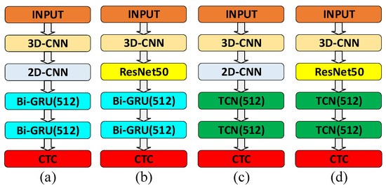
Figure 6.
Diagrams of ablation experiments with different architectures. (a) 3D-2D-CNN-BGRU-CTC, (b) 3D-ResNet50-BGRU-CTC, (c) 3D-2D-CNN-TCN-CTC, (d) 3D-ResNet50-TCN-CTC.
We trained 45 epochs for each architecture, and calculate its training and evaluate loss under one epoch for each iteration. To describe the differences more vividly, we use curve graphs to represent these data, as shown in Figure 7 and Figure 8. From the figure, it can be seen that the losses of the four architectures are steadily decreasing until they approach a fixed value. Comparing the 3D-2D-CNN-BGRU-CTC and 3D-ResNet50-BGRU-CTC architectures, the 3D-2D-CNN-TCN-CTC and 3D-ResNet50-TCN-CTC architectures converge faster, there is no vanishing gradient, and minimal losses can be achieved. Comparing the 3D-2D-CNN-BGRU-CTC and 3D-2D-CNN-TCN-CTC architectures, the 3D-ResNet50-BGRU-CTC and 3D-ResNet50-TCN-CTC architectures use efficient feature extractors, so the final loss is relatively small, and the accuracy rate is relatively improved.
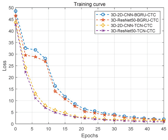
Figure 7.
Training curve. Training Loss curves with epochs for four different architectures. Epoch and Loss in the figure, respectively, represent the number of Epoch and the Loss reached under the Epoch.
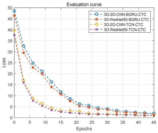
Figure 8.
Evaluation curve. Evaluation Loss curves with epochs for four different architectures. Epoch and Loss in the figure respectively represent the number of Epoch and the Loss reached under the Epoch.
The above experiments prove that the proposed architecture has back propagation paths in different sequence time directions, thereby avoiding gradient explosion/ disappearance in RNNs (such as LSTM, GRU). In addition, the use of an efficient feature extractor combining 3D and ResNet50 [37] convolutional networks has improved the performance of our architecture.
6. Results
Comparing the [22,23,24,30] architectures, the proposed architecture achieves the state-of-the-art accuracy (Acc = 1 − WER). We have presented the detailed report data in Table 3. In the table, ‘NA’ indicates that the method did not evaluate the evaluation protocol, ‘unseen’ indicates that the training data are separated from the evaluation data, and ‘seen’ is the opposite by coincidence.
Table 3.
Performance on the GRID dataset.
We also present statistics of the performance data of the four architectures for 3D-2D-CNN-BGRU-CTC, 3D-ResNet50-BGRU-CTC, 3D-2D-CNN-TCN-CTC, and 3D-ResNet50-TCN-CTC on the GRID dataset [29]. The experimental results are shown in Table 4. 3D-ResNet50-TCN-CTC is our proposed architecture, which achieves the state-of-the-art accuracy on each evaluation protocol. The experimental results show that an efficient feature extractor and high-performance TCN [36] as a feature learner have apparent practical effects for accelerating model convergence, improving performance accuracy, and reducing training memory requirements.
Table 4.
Comparison between different architectures.
7. Conclusions
This paper proposed an efficient end-to-end sentence-level lipreading architecture, using an efficient feature extractor that combines 3D convolution and ResNet50 [37], and replacing the traditional recurrent neural network with a Temporal Convolutional Network (TCN) [36]. Finally, an end-to-end sentence-level lipreading architecture was trained using the CTC objective function [17]. The proposed architecture overcomes the difficulties of slow convergence, disappearing gradient, and poor performance. Experiments on the GRID dataset show that, compared with the state-of-the-art method, the performance accuracy increase by 2.4%, and the convergence speed increase by 50%.
We divide our future work into three directions: first, the CTC objective function [17] used by the proposed architecture is based on independent conditional probability. Therefore, our research will focus on proposing a solution to this defect. Secondly, we can fully integrate voice features and visual features to seek further breakthroughs in performance. Finally, due to the shortcomings of long text samples in lipreading, designing a set of efficient and long-term dependent decoders is our future research direction.
Author Contributions
Conceptualization, T.Z., L.H. and G.F.; methodology, T.Z. and L.H.; software, L.H. and X.L.; validation, T.Z., L.H. and G.F.; formal analysis, L.H.; investigation, T.Z. and L.H.; resources, T.Z.; data curation, L.H.; writing—original draft preparation, T.Z. and L.H.; writing—review and editing, L.H. and X.L.; visualization, T.Z. and L.H.; supervision, T.Z.; project administration, L.H.; funding acquisition, T.Z. All authors have read and agreed to the published version of the manuscript.
Funding
This research was funded by the Zhejiang Lab’s International Talent Fund for Young Professionals.
Institutional Review Board Statement
Not applicable.
Informed Consent Statement
Informed consent was obtained from all subjects involved in the study.
Data Availability Statement
The data that support the findings of this study are available at http://spandh.dcs.shef.ac.uk/gridcorpus (accessed on 21 August 2020) [29]. These data were derived from the following resources available in the public domain: [https://zenodo.org/record/3625687#.YMMRmfkzY2w (accessed on 12 July 2020), http://spandh.dcs.shef.ac.uk/gridcorpus/ (accessed on 2 September 2020)].
Acknowledgments
The authors would like to acknowledge the high-performance graphics card provided by the DSP Laboratory of School of Electrical and Information Engineering, Tianjin University and the language support services provided by BiYun Ding.
Conflicts of Interest
The authors declare no conflict of interest.
References
- Potamianos, G.; Neti, C.; Gravier, G.; Garg, A.; Senior, A.W. Recent advances in the automatic recognition of audiovisual speech. Proc. IEEE 2003, 91, 1306–1326. [Google Scholar] [CrossRef]
- Akhtar, Z.; Micheloni, C.; Foresti, G.L. Biometric liveness detection: Challenges and research opportunities. IEEE Secur. Priv. 2015, 13, 63–72. [Google Scholar] [CrossRef]
- Rekik, A.; Ben-Hamadou, A.; Mahdi, W. Human machine interaction via visual speech spotting. In International Conference on Advanced Concepts for Intelligent Vision Systems; Springer: Berlin/Heidelberg, Germany, 2015; pp. 566–574. [Google Scholar]
- Wu, D.; Ruan, Q. Lip reading based on cascade feature extraction and HMM. In Proceedings of the 2014 12th International Conference on Signal Processing (ICSP), Hangzhou, China, 19–23 October 2014; pp. 1306–1310. [Google Scholar]
- Morade, S.S.; Patnaik, S. Lip reading using dwt and lsda. In Proceedings of the 2014 IEEE International Advance Computing Conference (IACC), Gurgaon, India, 21–22 February 2014; pp. 1013–1018. [Google Scholar]
- Dupont, S.; Luettin, J. Audio-visual speech modeling for continuous speech recognition. IEEE Trans. Multimed. 2000, 2, 141–151. [Google Scholar] [CrossRef]
- Zhou, Z.; Zhao, G.; Hong, X.; Pietikäinen, M. A review of recent advances in visual speech decoding. Image Vis. Comput. 2014, 32, 590–605. [Google Scholar] [CrossRef]
- Noda, K.; Yamaguchi, Y.; Nakadai, K.; Okuno, H.G.; Ogata, T. Audio-visual speech recognition using deep learning. Appl. Intell. 2015, 42, 722–737. [Google Scholar] [CrossRef] [Green Version]
- Petridis, S.; Pantic, M. Deep complementary bottleneck features for visual speech recognition. In Proceedings of the 2016 IEEE International Conference on Acoustics, Speech and Signal Processing (ICASSP), Shanghai, China, 20–25 March 2016; pp. 2304–2308. [Google Scholar]
- Geng, Y.; Zhang, G.; Li, W.; Gu, Y.; Liang, R.Z.; Liang, G.; Wang, J.; Wu, Y.; Patil, N.; Wang, J.Y. A novel image tag completion method based on convolutional neural transformation. In International Conference on Artificial Neural Networks; Springer: Berlin/Heidelberg, Germany, 2017; pp. 539–546. [Google Scholar]
- Miao, S.; Wang, Z.J.; Liao, R. A CNN regression approach for real-time 2D/3D registration. IEEE Trans. Med. Imaging 2016, 35, 1352–1363. [Google Scholar] [CrossRef]
- Wu, J.; Abdel-Fatah, E.E.; Mahfouz, M.R. Fully automatic initialization of two-dimensional–three-dimensional medical image registration using hybrid classifier. J. Med. Imaging 2015, 2, 024007. [Google Scholar] [CrossRef] [Green Version]
- Ding, M.; Fan, G. Articulated and generalized gaussian kernel correlation for human pose estimation. IEEE Trans. Image Process. 2015, 25, 776–789. [Google Scholar] [CrossRef] [PubMed]
- Wang, X.; Pollock, L.; Vijay-Shanker, K. Automatic segmentation of method code into meaningful blocks to improve readability. In Proceedings of the 2011 18th Working Conference on Reverse Engineering, Limerick, Ireland, 17–20 October 2011; pp. 35–44. [Google Scholar]
- Stafylakis, T.; Khan, M.H.; Tzimiropoulos, G. Pushing the boundaries of audiovisual word recognition using residual networks and LSTMs. Comput. Vis. Image Underst. 2018, 176, 22–32. [Google Scholar] [CrossRef] [Green Version]
- Petridis, S.; Wang, Y.; Ma, P.; Li, Z.; Pantic, M. End-to-end visual speech recognition for small-scale datasets. Pattern Recognit. Lett. 2020, 131, 421–427. [Google Scholar] [CrossRef] [Green Version]
- Graves, A. Connectionist temporal classification: Labelling unsegmented sequence data with recurrent neural networks. In Proceedings of the 23rd International Conference on Machine Learning, Pittsburgh, PA, USA, 25–29 June 2006. [Google Scholar]
- Graves, A.; Jaitly, N. Towards end-to-end speech recognition with recurrent neural networks. In Proceedings of the International Conference on Machine Learning, Beijing, China, 21–26 June 2014; pp. 1764–1772. [Google Scholar]
- Amodei, D.; Ananthanarayanan, S.; Anubhai, R.; Bai, J.; Battenberg, E.; Case, C.; Casper, J.; Catanzaro, B.; Cheng, Q.; Chen, G.; et al. Deep speech 2: End-to-end speech recognition in english and mandarin. In Proceedings of the International Conference on Machine Learning, New York, NY, USA, 14–24 June 2016; pp. 173–182. [Google Scholar]
- Bahdanau, D.; Cho, K.; Bengio, Y. Neural machine translation by jointly learning to align and translate. arXiv 2014, arXiv:1409.0473. [Google Scholar]
- Chan, W.; Jaitly, N.; Le, Q.V.; Vinyals, O. Listen, attend and spell. arXiv 2015, arXiv:1508.01211. [Google Scholar]
- Assael, Y.M.; Shillingford, B.; Whiteson, S.; De Freitas, N. Lipnet: End-to-end sentence-level lipreading. arXiv 2016, arXiv:1611.01599. [Google Scholar]
- Xu, K.; Li, D.; Cassimatis, N.; Wang, X. LCANet: End-to-end lipreading with cascaded attention-CTC. In Proceedings of the 2018 13th IEEE International Conference on Automatic Face & Gesture Recognition (FG 2018), Xi’an, China, 15–19 May 2018; pp. 548–555. [Google Scholar]
- Margam, D.K.; Aralikatti, R.; Sharma, T.; Thanda, A.; Roy, S.; Venkatesan, S.M. LipReading with 3D-2D-CNN BLSTM-HMM and word-CTC models. arXiv 2019, arXiv:1906.12170. [Google Scholar]
- Krizhevsky, A.; Sutskever, I.; Hinton, G.E. Imagenet classification with deep convolutional neural networks. Commun. ACM 2017, 60, 84–90. [Google Scholar] [CrossRef]
- Karpathy, A.; Toderici, G.; Shetty, S.; Leung, T.; Sukthankar, R.; Li, F.-F. Large-scale video classification with convolutional neural networks. In Proceedings of the IEEE Conference on Computer Vision and Pattern Recognition, Columbus, OH, USA, 23–28 June 2014; pp. 1725–1732. [Google Scholar]
- Schuster, M.; Paliwal, K.K. Bidirectional recurrent neural networks. IEEE Trans. Signal Process. 1997, 45, 2673–2681. [Google Scholar] [CrossRef] [Green Version]
- Hochreiter, S.; Schmidhuber, J. Long short-term memory. Neural Comput. 1997, 9, 1735–1780. [Google Scholar] [CrossRef] [PubMed]
- Cooke, M.; Barker, J.; Cunningham, S.; Shao, X. An audio-visual corpus for speech perception and automatic speech recognition. J. Acoust. Soc. Am. 2006, 120, 2421–2424. [Google Scholar] [CrossRef] [Green Version]
- Chung, J.S.; Senior, A.; Vinyals, O.; Zisserman, A. Lip reading sentences in the wild. In Proceedings of the 2017 IEEE Conference on Computer Vision and Pattern Recognition (CVPR), Honolulu, HI, USA, 21–26 July 2017; pp. 3444–3453. [Google Scholar]
- Chung, J.S.; Zisserman, A. Out of time: Automated lip sync in the wild. In Asian Conference on Computer Vision; Springer: Berlin/Heidelberg, Germany, 2016; pp. 251–263. [Google Scholar]
- Chung, J.S.; Zisserman, A. Lip reading in the wild. In Asian Conference on Computer Vision; Springer: Berlin/Heidelberg, Germany, 2016; pp. 87–103. [Google Scholar]
- Chen, Z.; Droppo, J.; Li, J.; Xiong, W. Progressive joint modeling in unsupervised single-channel overlapped speech recognition. IEEE/ACM Trans. Audio Speech Lang. Process. 2017, 26, 184–196. [Google Scholar] [CrossRef]
- Erdogan, H.; Hayashi, T.; Hershey, J.R.; Hori, T.; Hori, C.; Hsu, W.N.; Kim, S.; Le Roux, J.; Meng, Z.; Watanabe, S. Multi-channel speech recognition: Lstms all the way through. In Proceedings of the CHiME-4 Workshop, San Francisco, CA, USA, 19 August 2016; pp. 1–4. [Google Scholar]
- Yin, W.; Kann, K.; Yu, M.; Schütze, H. Comparative study of cnn and rnn for natural language processing. arXiv 2017, arXiv:1702.01923. [Google Scholar]
- Bai, S.; Kolter, J.Z.; Koltun, V. An empirical evaluation of generic convolutional and recurrent networks for sequence modeling. arXiv 2018, arXiv:1803.01271. [Google Scholar]
- He, K.; Zhang, X.; Ren, S.; Sun, J. Deep residual learning for image recognition. In Proceedings of the IEEE Conference on Computer Vision and Pattern Recognition, Las Vegas, NV, USA, 27–30 June 2016; pp. 770–778. [Google Scholar]
- Matthews, I.; Potamianos, G.; Neti, C.; Luettin, J. A comparison of model and transform-based visual features for audio-visual LVCSR. In Proceedings of the IEEE International Conference on Multimedia and Expo, Tokyo, Japan, 22–25 August 2001; p. 210. [Google Scholar]
- Sui, C.; Bennamoun, M.; Togneri, R. Listening with your eyes: Towards a practical visual speech recognition system using deep boltzmann machines. In Proceedings of the IEEE International Conference on Computer Vision, Santiago, Chile, 7–13 December 2015; pp. 154–162. [Google Scholar]
- Chung, J.; Gulcehre, C.; Cho, K.; Bengio, Y. Empirical evaluation of gated recurrent neural networks on sequence modeling. arXiv 2014, arXiv:1412.3555. [Google Scholar]
- Melis, G.; Dyer, C.; Blunsom, P. On the state of the art of evaluation in neural language models. arXiv 2017, arXiv:1707.05589. [Google Scholar]
- Gehring, J.; Auli, M.; Grangier, D.; Yarats, D.; Dauphin, Y.N. Convolutional sequence to sequence learning. arXiv 2017, arXiv:1705.03122. [Google Scholar]
- Kalchbrenner, N.; Espeholt, L.; Simonyan, K.; Oord, A.V.D.; Graves, A.; Kavukcuoglu, K. Neural machine translation in linear time. arXiv 2016, arXiv:1610.10099. [Google Scholar]
- Dauphin, Y.N.; Fan, A.; Auli, M.; Grangier, D. Language modeling with gated convolutional networks. In Proceedings of the International Conference on Machine Learning, Sydney, Australia, 6–11 August 2017; pp. 933–941. [Google Scholar]
- Ioffe, S.; Szegedy, C. Batch normalization: Accelerating deep network training by reducing internal covariate shift. arXiv 2015, arXiv:1502.03167. [Google Scholar]
- Glorot, X.; Bordes, A.; Bengio, Y. Deep sparse rectifier neural networks. In Proceedings of the Fourteenth International Conference on Artificial Intelligence and Statistics, Lauderdale, FL, USA, 11–13 April 2011; pp. 315–323. [Google Scholar]
- He, K.; Zhang, X.; Ren, S.; Sun, J. Identity mappings in deep residual networks. In European Conference on Computer Vision; Springer: Berlin/Heidelberg, Germany, 2016; pp. 630–645. [Google Scholar]
- Srivastava, N.; Hinton, G.; Krizhevsky, A.; Sutskever, I.; Salakhutdinov, R. Dropout: A simple way to prevent neural networks from overfitting. J. Mach. Learn. Res. 2014, 15, 1929–1958. [Google Scholar]
- Wand, M.; Koutník, J.; Schmidhuber, J. Lipreading with long short-term memory. In Proceedings of the 2016 IEEE International Conference on Acoustics, Speech and Signal Processing (ICASSP), Shanghai, China, 20–25 March 2016; pp. 6115–6119. [Google Scholar]
- Sagonas, C.; Tzimiropoulos, G.; Zafeiriou, S.; Pantic, M. 300 faces in-the-wild challenge: The first facial landmark localization challenge. In Proceedings of the IEEE International Conference on Computer Vision Workshops, Sydney, Australia, 2–8 December 2013; pp. 397–403. [Google Scholar]
- Abadi, M.; Barham, P.; Chen, J.; Chen, Z.; Davis, A.; Dean, J.; Devin, M.; Ghemawat, S.; Irving, G.; Isard, M.; et al. Tensorflow: A system for large-scale machine learning. In Proceedings of the 12th {USENIX} Symposium on Operating Systems Design and Implementation ({OSDI} 16), Savannah, GA, USA, 2–4 November 2016; pp. 265–283. [Google Scholar]
- Kingma, D.P.; Ba, J. Adam: A method for stochastic optimization. arXiv 2014, arXiv:1412.6980. [Google Scholar]
Publisher’s Note: MDPI stays neutral with regard to jurisdictional claims in published maps and institutional affiliations. |
© 2021 by the authors. Licensee MDPI, Basel, Switzerland. This article is an open access article distributed under the terms and conditions of the Creative Commons Attribution (CC BY) license (https://creativecommons.org/licenses/by/4.0/).