Stamping Tool Conditions Diagnosis: A Deep Metric Learning Approach

Abstract

Stamping processes remain crucial in manufacturing processes; therefore, diagnosing the condition of stamping tools is critical. One of the challenges in diagnosing stamping tool conditions is that traditionally, the tools need to be visually checked, and the production processes thus need to be halted. With the development of Industry 4.0, intelligent monitoring systems have been developed by using accelerometers and algorithms to diagnose the wear classification of stamping tools. Although several deep learning models such as the convolutional neural network (CNN), auto encoder (AE), and recurrent neural network (RNN) models have demonstrated promising results for classifying complex signals including accelerometer signals, the practicality of those methods are restricted due to the flexibility of adding new classes and low accuracy when faced to low numbers of samples per class. In this study, we applied deep metric learning (DML) methods to overcome these problems. DML involves extracting meaningful features using feature extraction modules to map inputs into embedding features. We compared the probability method, the contrastive method, and a triplet network to determine which method was most suitable for our case. The experimental results revealed that, compared with other models, a triplet network can be more effectively trained with limited training data. The triplet network demonstrated the best test results of the compared methods in the noised test data. Finally, when tested using unseen class, the triplet network and the probability method demonstrated similar results.

1. Introduction

The metal stamping process remains one of the most common processes in manufacturing and is still being used by major industries, including the automotive, aerospace, and consumer appliances industries [1]. Therefore, the stamping process must be monitored and diagnosed to ensure that every product meets the required quality standards. A crucial component requiring diagnosis is the tool die, the quality of which can greatly affect the outcome of a product. One of the challenges in diagnosing stamping tool conditions is that, traditionally, the tools need to be visually checked and the production processes thus need to be halted. Following the trend of Industry 4.0, automation in stamping processes has triggered the use of online intelligent condition monitoring systems, which are crucial for improving the productivity and availability of production systems. Today’s advanced sensor technology pays attention to and incorporates numerous mechanical properties such as vibration, strain, and displacement to monitor the conditions of manufacturing processes [2], however acquiring the mechanical properties from the tool is only the beginning of diagnosing its condition. Nonetheless, these data need to be analyzed and processed before we able to diagnose tool condition. The advancement of Industry 4.0 also accelerates the research and development of machine learning, which is extremely helpful to analyze the non-linear data that are being used to monitor stamping process.

Traditional signal processing and conventional machine learning methods have been employed in several studies on the stamping processes and tool diagnosis. For example, Ge [3] used the hidden Markov model, Bassiuny [4] used empirical mode decomposition combined with learning vector quantization, and other researchers [5,6,7,8] have employed audio and autoencoders (AEs). Furthermore, Ge [9] used support-vector machines, and Zhang [10] used a wavelet transform combined with semi-supervised clustering. Zhou [11] proposed a recurrence plot based on waveform signals to monitor the progressive stamping process. Sah [12] used an embedded pressure sensor inside a tool die to monitor the stamping process. However, these studies had several shortcomings: (1) the manual feature extraction process can be tedious, requiring substantial time and effort; (2) manually extracted features do not adapt well to evolving conditions and scenarios during the stamping process.

Deep learning methods that have been developed have been applied to intelligent condition diagnosis, achieving favorable results [13] using architectures such as convolutional neural networks (CNNs) [14,15,16,17,18], AEs [19,20,21,22,23], and recurrent neural networks [24,25,26,27,28]. CNNs, which employ neural nodes as a type of filter, enable deep learning structures to extract features from complex and highly nonlinear signals. In our previous work [29], a CNN was used to evaluate the condition of a stamping tool, achieving favorable results; however, several problems remain to be resolved. First, to add a new class, the model must be retrained, which requires a high computational cost. Second, to retrain the model, sufficient data for each class and the retraining process must first be obtained, which requires subsequent downtime. Bromley [30] proposed a network architecture called a Siamese network, that has two inputs and compares the similarity between these inputs; the deep metric learning (DML) [31] algorithm has same principle, but to produce that similarity, a DML uses deep learning to extract features to be compared, using this technique it provides several advantages over traditional deep learning methods. First, the feature extraction module (FEM) (i.e., CNN), with all its benefits, is still used to extract features. Second, rather than learning to discover a class, DML identifies similarities between two objects, thereby we can dynamically add a new, unseen class without the requirement for model retraining.

At its core, DML is a W projection matrix [32]; the FEM transforms objects into the W projection matrix and then learns according to its projection matrix similarity. The distances between these projection matrices demonstrate the similarities of the objects. A contrastive loss method [33] can be used to minimize the distance between the projection matrices for same samples and maximize it for different samples. A selection of samples for batches in training [34] is also can contribute to a better result in DML.

On the basis of its advantages, DML has been used to develop robust algorithms that respond to changes in working conditions. Previously, Li et al. [35] proposed novel deep distance metric learning combined with representation clustering to diagnose a rolling element bearing with limited data required to learn. In addition, Wang et al. [36] used deep metric learning combined with meta-learning to diagnose bearing faults with few-shot samples. On the other hand, Zhang et al. [37] proposed deep metric learning with a probability method to diagnose faults in bearings using a limited number of samples. Liu et al. [38] proposed a similar method to Zhang. It was used to classify Raman spectroscopy and able to add new classes. In the method prosed by Zhang et al. [37], the DML was able to recognize an unseen class, whereas Liu et al. [38] proposed a model able to dynamically add a class with as few as one example. The DML itself has several variations of techniques to implement ranging from batch selections to loss functions, and its application can be found in many fields, such as facial or signal recognition [33,34,35,36,37,38]. However, to our knowledge, a thorough investigation involving batch selection strategies and loss functions to determine the most effective DML method for stamping tool condition diagnosis has not been conducted.

Herein, we propose a solution for stamping tool condition diagnosis that offers improvements over the method introduced in our previous work [29], the main improvement that we aim to achieve is the flexibility of adding new class while still retaining the advantages gained from the previous work. The solution is based on the incorporation of DML with several distance metric loss and batch strategies. The contributions of this study are as follows:

• We developed a DML method for stamping tool condition diagnosis that incorporates several distance metric loss and batch strategies.
• We investigated the performance of each distance metric loss and batch selection method.
• We investigated the robustness of each loss and mining method based on the degree of training data variation, noise injection, and capability of adding new classes.

The remainder of this paper is organized as follows: Section II describes metric learning and DML. Section III presents the proposed experiments, their results, and a discussion. Finally, section IV presents the research conclusions.

2. Materials and Methods

2.1. Metric Learning and Deep Metric Learning (DML)

Metric learning is a type of machine learning based on the distances between objects, where the distance itself represents a similarity measurement. Suppose a given dataset $X$ with $X \in {ℝ}^{N\times D}$, where $x_i \in {ℝ}^N$ is the $i$th datum and $D$ is the total number of data samples; next, set $X^{\prime }$ as the mapping of $X$ with the distance function over $d_M:X^{\prime }\times X^{\prime }\in {ℝ}^m$. This metric or distance function must satisfy the following axioms:

(1)

Negativity: $d_M\left(x_i,x_j\right)\ge 0$,

(2)

Symmetry: $d_M\left(x_i,x_j\right)=d\left(x_j,x_i\right)$,

(3)

Triangular inequality: $d_M\left(x_i,x_j\right)\le d\left(x_i,x_k\right)+d\left(x_j,x_k\right)$,

(4)

Identity of indiscernible: $d_M\left(x_i,x_j\right)iffi=j$.

A pair $\left(X^{\prime },d_M\right)$ in which $X^{\prime }$ is a set and $d$ is a metric in the metric space. Although the metric obeys the five aforementioned axioms, metric learning ignores the final axiom (triangular inequality). Therefore, the properties of $\left(X^{\prime },d_M\right)$ change from metric space to pseudometric space. Pseudometrics are sometimes referred to as metrics in metric learning. The distance metric itself is calculated as follows:

$$d_M=\sqrt{{\left(x_i-x_j\right)}^{T}M\left(x_i-x_j\right)}$$

(1)

where $M$ must be a symmetrical and positive semidefinite matrix; if $M=W^{T}W$, then function (1) can be written as function (2):

$$d_M=\sqrt{{\left(x_i-x_j\right)}^T{W}^{T}W\left(x_i-x_j\right)}$$

(2)

$$d_M{}^2=\Vert W{x}_i-W{x}_j\Vert {}_2^2$$

(3)

$$d_M=\Vert x_i^{\prime }-x_j^{\prime }{\Vert }_2$$

(4)

The distance $d_s$ is the Eucledian distance of the feature representation vectors $x_i^{\prime }=W{x}_i$ and $W{x}_j$. The main objective of metric learning is training through the mapping function $f$; if $f:X\to {ℝ}^n$ is substituted into function (4), then it becomes function (5):

$$d_M=\Vert f\left(x_i\right)-f{\left(x_j\right)\Vert }_2$$

(5)

Training $f$ under various loss functions and other boundaries thus becomes the clear purpose of metric learning. Because deep learning models can be trained to learn linear or nonlinear problems, they can be used to map data points into feature space, and the weight and biases in deep learning architectures can be trained using various loss functions incorporating distance metric (5). The two most common architectures used for DML applications are Siamese neural networks and triplet networks.

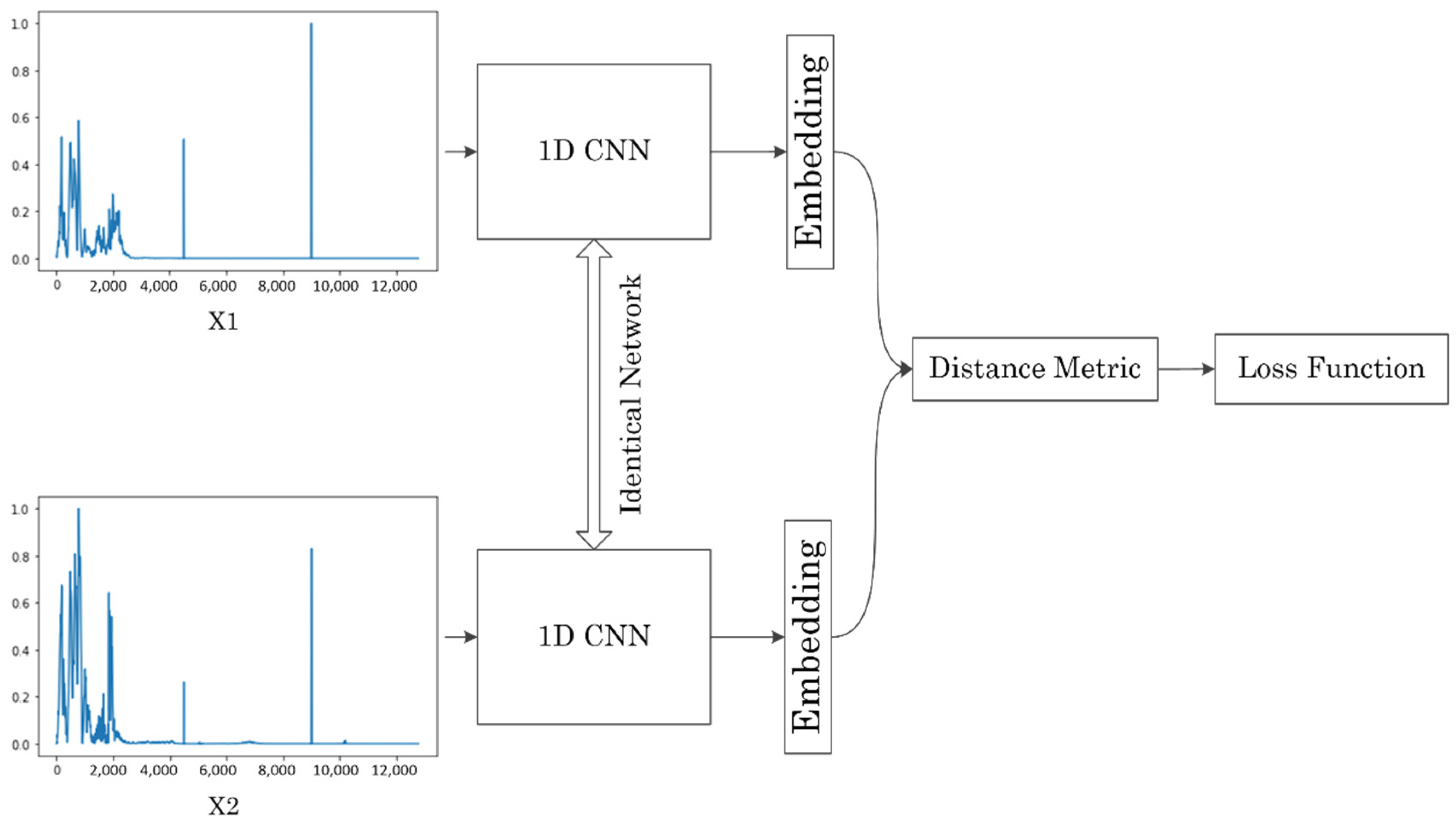
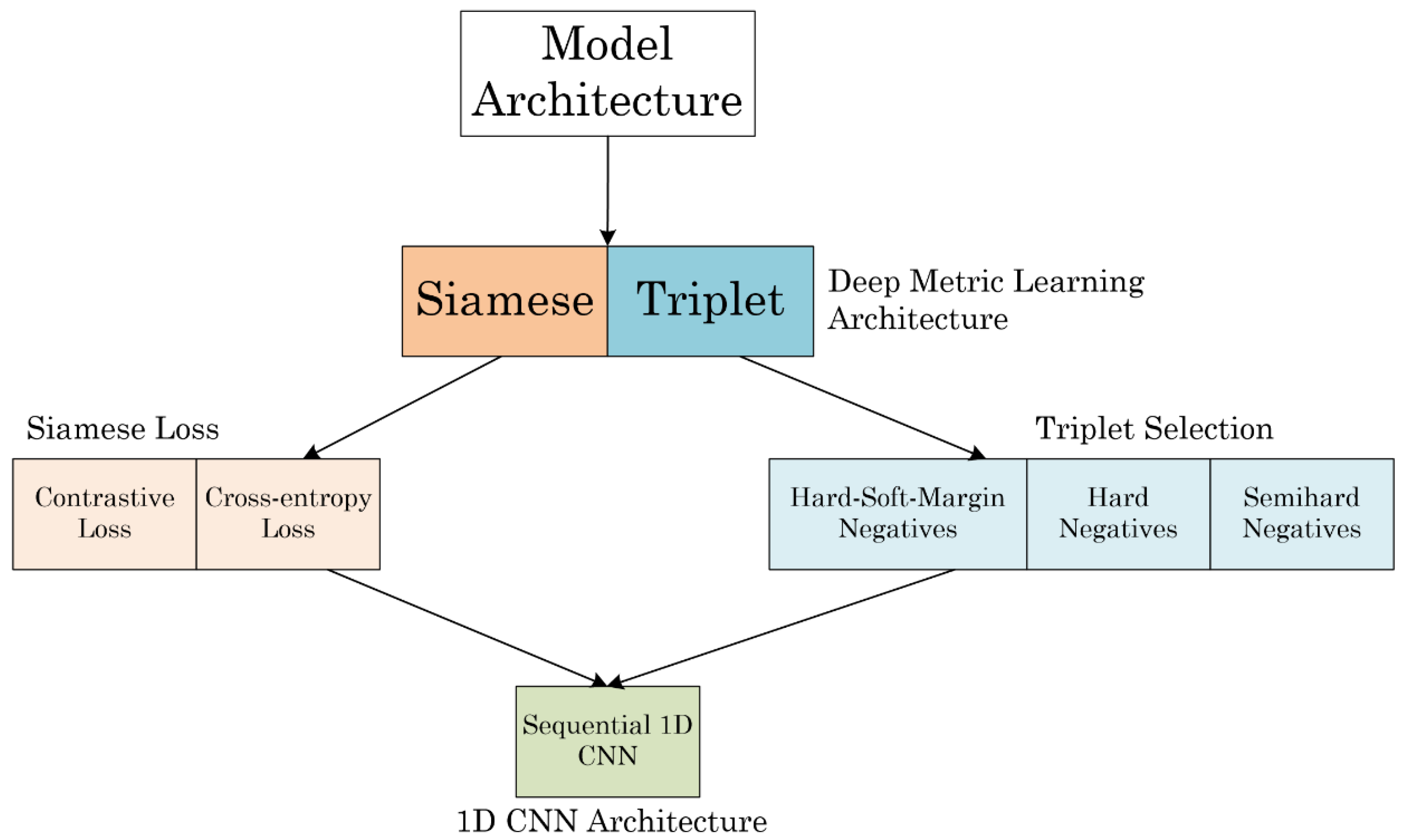
2.2. Siamese Neural Network

A Siamese neural network [30] uses a single FEM, but it is used to map two data inputs into a feature space. The term “Siamese” reflects the nature of the shared neural network. Figure 1 presents an architecture of a Siamese neural network, where two samples are fed into a network in which two identical CNNs act as an FEM; they are then transformed into a feature space. After a feature representation is created, several methods can be used to train the CNN, namely the probability method [38] and the contrastive method [33].

2.2.1. Probability Method

Suppose we already have a feature representation from input $\left(x_1,x_2\right)$ extracted using two FEMs. If FEM is denoted as a function $f$, then the distance metric can be obtained using function (5), thus yielding function (6).

$$d_M\left(x_1,x_2\right)=\Vert f\left(x_1\right)-f{\left(x_2\right)\Vert }_2$$

(6)

The output from the distance metric is then converted into the probability of the two samples being the same. This probability can be computed using the sigmoid function (7):

$$P\left(x_1,x_2\right)=\sigma \left(d_M\left(x_1,x_2\right)\right)$$

(7)

Let $t=y\left(x_1,x_2\right)$ be the binary label for inputs $x_1$ and $x_2$. Let $t_i=1$ if $x_{i }$ and $x_j$ are from the same class; otherwise, $t_i=0$. Because the output is a probability problem, regularized cross-entropy is used as loss function (8):

$${ℒ}_{XENT}\left(x_1,x_2,t\right)=t\log \left(P\left(x_1,x_2\right)\right)+\left(1-t\right)\log \left(1-P\left(x_1,x_2\right)\right)$$

(8)

2.2.2. Contrastive Method

The contrastive method minimizes the metric distance between inputs of the same class and dissociates the inputs of different classes. It still uses distance metric function (6), but instead of being used to activate another function, it is directly used in the loss function. A contrastive loss obtained using function (9) forces a positive pair to become closer to zero and pushes the negative pair with a degree of margin $\alpha$.

$${ℒ}_{CONT}\left(x_1,x_2,t\right)=t{d}_M\left(x_1,x_2\right)+\left(1-t\right)\max \left(0,\alpha -d_M\left(x_1,x_2\right)\right)$$

(9)

where $\alpha$ is the margin when the inputs are from different classes.

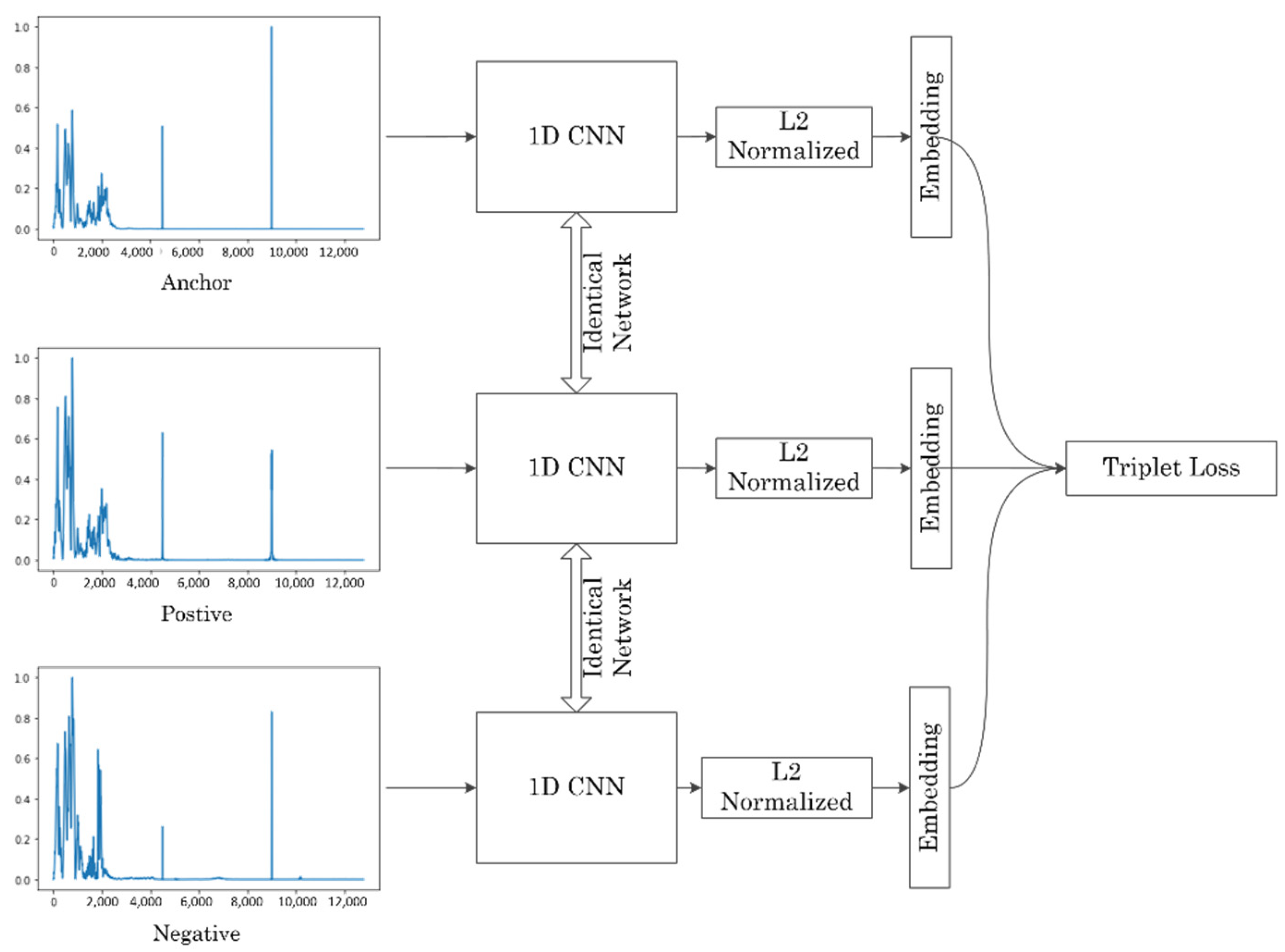
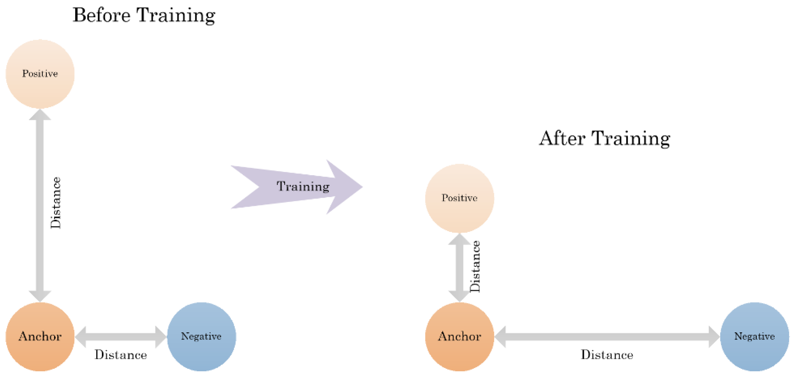
2.3. Triplet Network

Figure 2 presents a triplet network architecture. In this architecture, three identical CNNs are used as three FEMs; therefore, the weight, bias, and other parameters of the three CNNs are identical. Triplet datum $X_t$ is used as an input, and the given datum contains three sets of samples, namely anchor samples $x_a$, positive samples $x_p$, and negative samples $x_n$.

The $x_a$ and $x_p$ samples are from the same class, whereas the negative samples $x_n$ are from a different class than the $x_a$ samples. The purpose of triplet learning is to train the FEM (CNN) so that it can map a pseudometric space either close or far for positive and negative pairs, respectively (Figure 3).

2.3.1. Triplet Loss

The FEMs in the triplet training phase map data input into the embedding $f\left(x\right) \in {ℝ}^n$, which is a representation of Euclidean space of $n$-dimensional size. With (5), a distance metric can be calculated for a positive pair, as in (10), and for a negative pair, as in (11):

$$d_p\left(x_a,x_p\right)=\Vert f\left(x_a\right)-f{\left(x_p\right)\Vert }_2$$

(10)

$$d_n\left(x_a,x_n\right)=\Vert f\left(x_a\right)-f{\left(x_n\right)\Vert }_2$$

(11)

According to [39], a loss function for a triplet network using positive and negative pair distances is as follows:

$${ℒ}_{TRIP} \left(x_a,x_p,x_n\right)=\max \left(d_p\left(x_a,x_p\right)-d_n\left(x_a,x_n\right)+\alpha ,0\right)$$

(12)

where α is the margin added in the negative pair distance. This margin maintains a distance between the positive and negative groups, enabling the loss to push the negative group over the margin and away from the positive group.

2.3.2. Triplet Selection

Schroff et al. [34] proposed a problem for generating all possible triplets that may easily satisfy function (12). If these “easy triplets” fill most of the samples in the training data, then the result would be slower convergence; therefore, selecting the appropriate triplet data is crucial.

One method for selecting hard triplets to ensure fast convergence is to violate the constraint in function (12). However, “easy” and “hard” triplets must first be defined.

$$d_p\left(x_a,x_p\right)+\alpha <d_n\left(x_a,x_n\right)$$

(13)

An easy triplet (13) already fulfills the equation, and the model exerts less effort on learning. However, hard triplets (14) place the negative pair closer to the anchor than they place the positive pair, creating difficulty for the model in terms of learning.

$$d_n\left(x_a,x_n\right)<d_p\left(x_a,x_p\right)$$

(14)

Another type of triplet is a semihard triplet (15), in which the value of the negative pair is not smaller than that of the positive pair but falls between positive and negative both with and without a margin:

$$d_p\left(x_a,x_p\right)<d_n\left(x_a,x_n\right)<d_p\left(x_a,x_p\right)+\alpha$$

(15)

Figure 4 illustrates the differences between the types of triplets. Therein, the triplets are compared in terms of the distance between the negative and anchor. Each triplet yields a different effect on model training; that is, if the training batch contains an excessive number of easy triplets, then the model dose not learn effectively. However, an excessive number of hard triplets would generate a high loss and assign excessively high weights to mislabeled data.

Schroff et al. [34] also proposed online triplet mining, in which sets of triplets are generated before training. This method requires less effort, but may generate only easy or only hard triplets, which would necessitate the time-consuming process of manual data processing. Online triplet mining feeds a batch of training data, generates triplets by using all the samples in the batch, and then calculates the loss from every batch. Using this approach would increase the number of easy, hard, and semihard triplets included in every training batch.

2.3.3. Hard Triplet Soft Margin

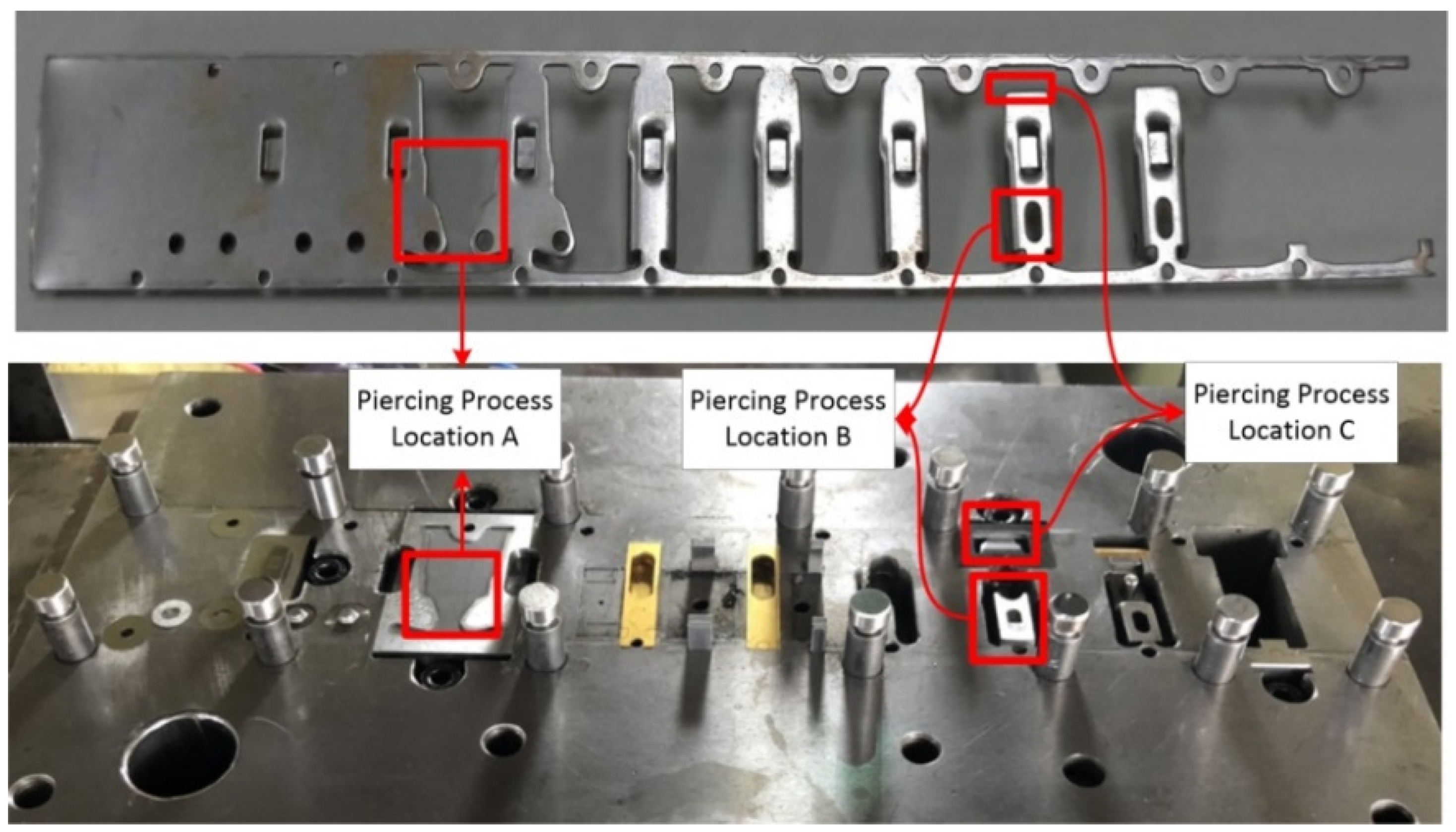
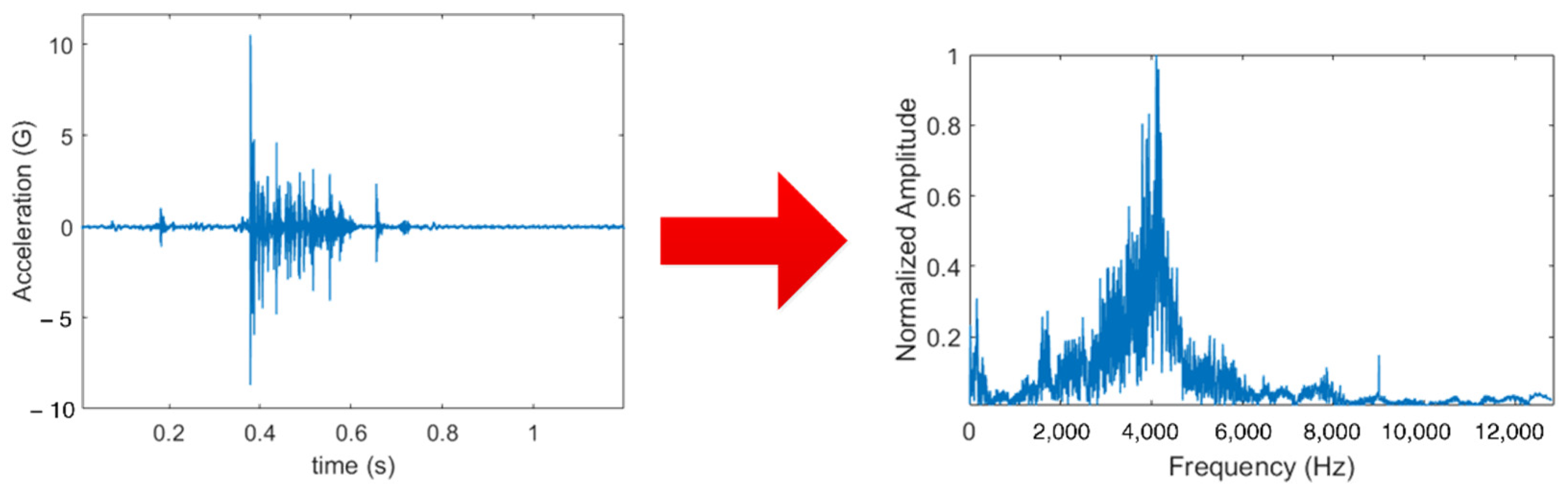
Hermans et al. [40] proposed a soft margin to replace a hinge function $\left[\mathsf{\alpha }+\circ \right]$ inside the triplet loss function (12), which is used to avoid overcorrection with the softplus function $\ln \left(1+\exp (\circ )\right)$for which practical implementation is expressed as $log1p$. They argue that samples from the same class can be beneficial for their case. The softplus function offers slow (exponential), rather than abrupt decay, using only margin $\mathsf{\alpha }$.

2.4. Dataset

The data set used in the current study was extensively used in our previous study [29]. It contains progressive stamping die vibration signals acquired using an accelerometer with a sampling rate of 25.6 kHz and an axis parallel to the stroke direction of the stamping machine. The stamping machine used (LCP-60H, Ingyu Machinery, Taiwan) had a capacity of 60 tons and an automatic sheet metal feeder. The sheet material used was SPCC steel with a thickness of 1.5 mm.

Three locations on the tool die as illustrated in Figure 5 were examined for two degrees of wear: mild and heavy. One set of healthy-condition samples was used as a reference.

In total, seven classes of wear were included in the stamping tool condition data set explained in

Table 1. Stamping tool condition data set.

Class Name	Class Type	Number of Samples
Healthy Condition	Class 1	280
Heavy Wear Position A	Class 2	280
Heavy Wear Position B	Class 3	280
Heavy Wear Position C	Class 4	280
Mild Wear Position A	Class 5	280
Mild Wear Position B	Class 6	280
Mild Wear Position C	Class 7	280

.

Data preprocessing was conducted for each vibration sample. First, each data sample was converted from time-based to frequency-based (frequency = 12.8 kHz). Second, each converted sample was normalized. The data transformation is presented in Figure 6.

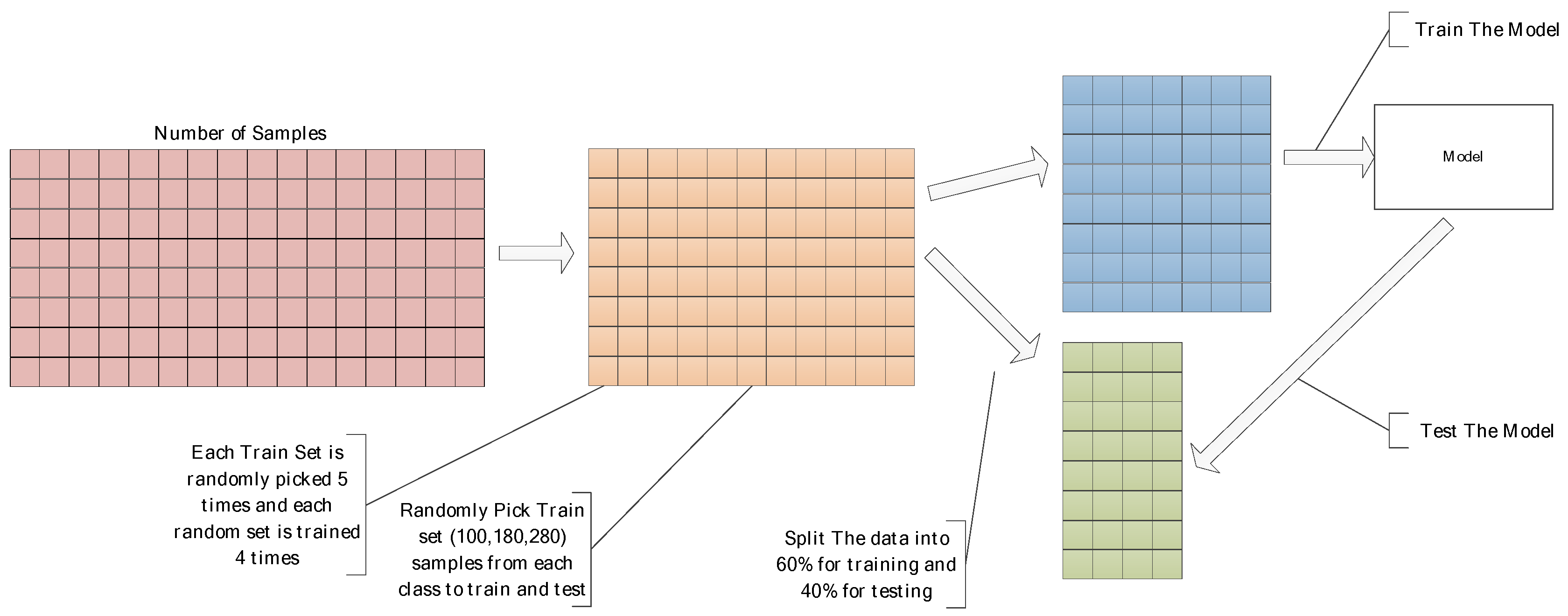
2.5. One-Shot K-Way Testing

For every test data sample $x_i^{\prime }\in X^{\prime }$, a support set S consisting of one $K$ number of test samples was created, in which only one sample, $x_j^{\prime }\in X^{\prime }$, was the same class as $x_i^{\prime }$. We then placed $x_j^{\prime }$ randomly inside S. Because every DML configuration is different, the probability method was used with a Siamese neural network to calculate the accuracy of each DML.

$$S=\left\{\left(x_1,y_1\right),\dots ,\left(x_K,y_K\right)\right\}$$

(16)

where $y$ is a distinct label of each data sample in support set S. Subsequently, each test sample can be classified using probabilistic function (7), in which the highest value indicates the sample most similar to test data sample $x^{\prime }$ as follows:

$$C_P\left(x^{\prime }, S\right)=\underset{c}{argmax}\left(P\left(x^{\prime },x_c\right)\right),x_c\in S$$

(17)

The accuracy is then calculated for the given test data set $X^{\prime }\in {ℝ}^{N\times D},$ where $N$ is the size of the test data set and $D$ is a dimension of data point $x_i^{\prime }$.

$$Accurac{y}_P=\frac{{{\displaystyle \sum }}_{i=1}^N{C}_P\left(x_i^{\prime }, S_i\right)}{N}$$

(18)

In terms of a Siamese neural network with contrastive loss and the triplet network, the greater the distance between classes, the more similar they are. Therefore, substituting (5) into (17) yields (19).

$$C_d\left(x^{\prime }, S\right)=\underset{c}{\mathrm{argmin}}\left(d\left(x^{\prime },x_c\right)\right),x_c\in S$$

(19)

The accuracy can then be calculated as (20).

$$Accurac{y}_d=\frac{{{\displaystyle \sum }}_{i=1}^N{C}_d\left(x_i^{\prime }, S_i\right)}{N}$$

(20)

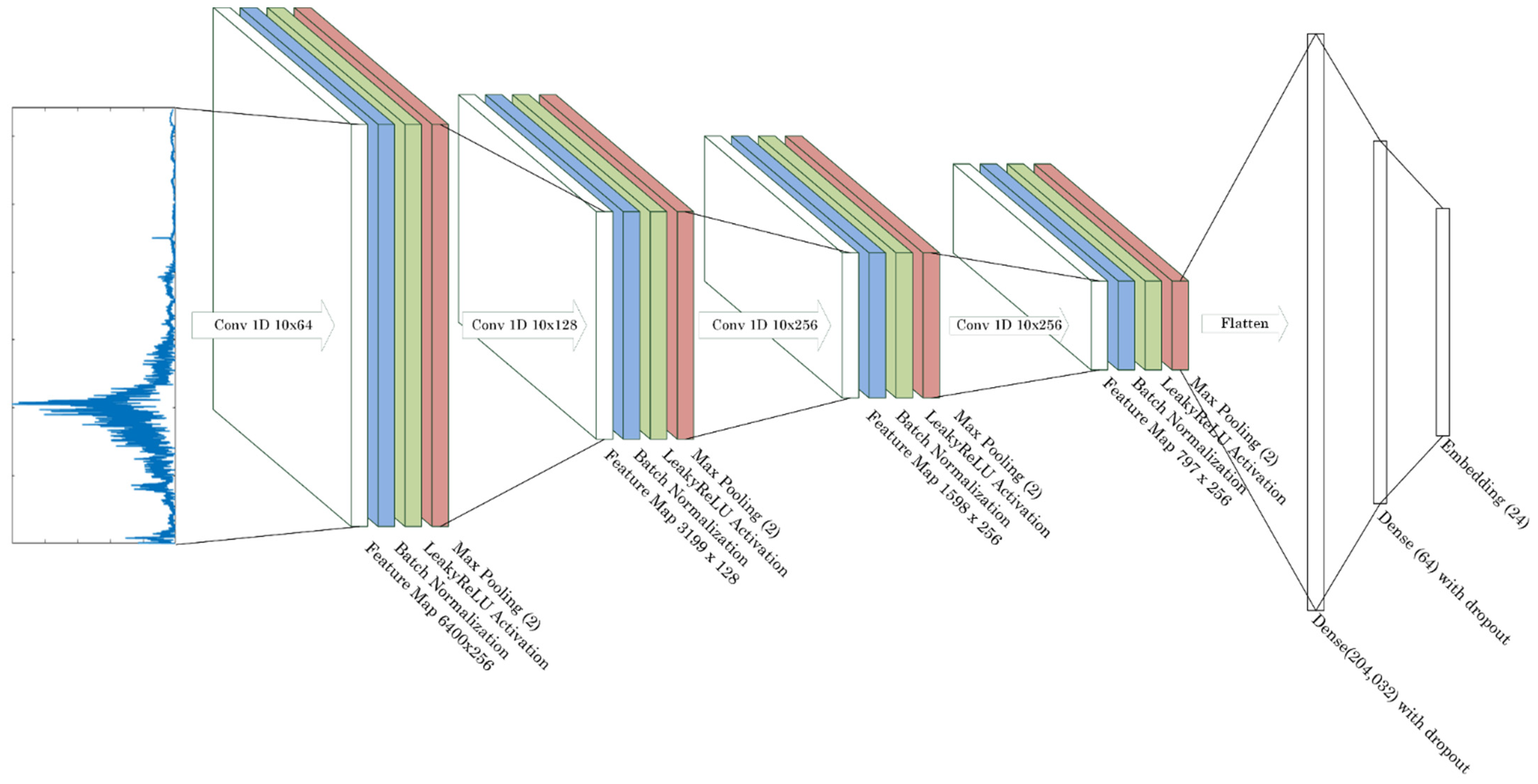
2.6. 1D CNN Architecture

Zhang et al. [38] proposed a wide first-layer kernel (WDCNN) to extract features from roller bearings. In their study, they used a Siamese network with a probability output. Their argument for using a wide first-layer kernel was that if the kernel was small then it could be disturbed by high frequency noise. In this study, we use normal kernel 1D CNN instead of WDCNN since our problem does not use time-based input. Figure 7 shows our proposed architecture.

3. Results and Discussions

Figure 8 presents the configurations of the five models developed in this study. All models were trained using Tensorflow 2.0 and an NVIDIA RTX2080 Ti GPU. A stochastic gradient descent with a fixed learning rate of 2 × 10⁻³ and a batch of 32 samples was used for all models. Identical deep CNNs were used as FEMs for all models.

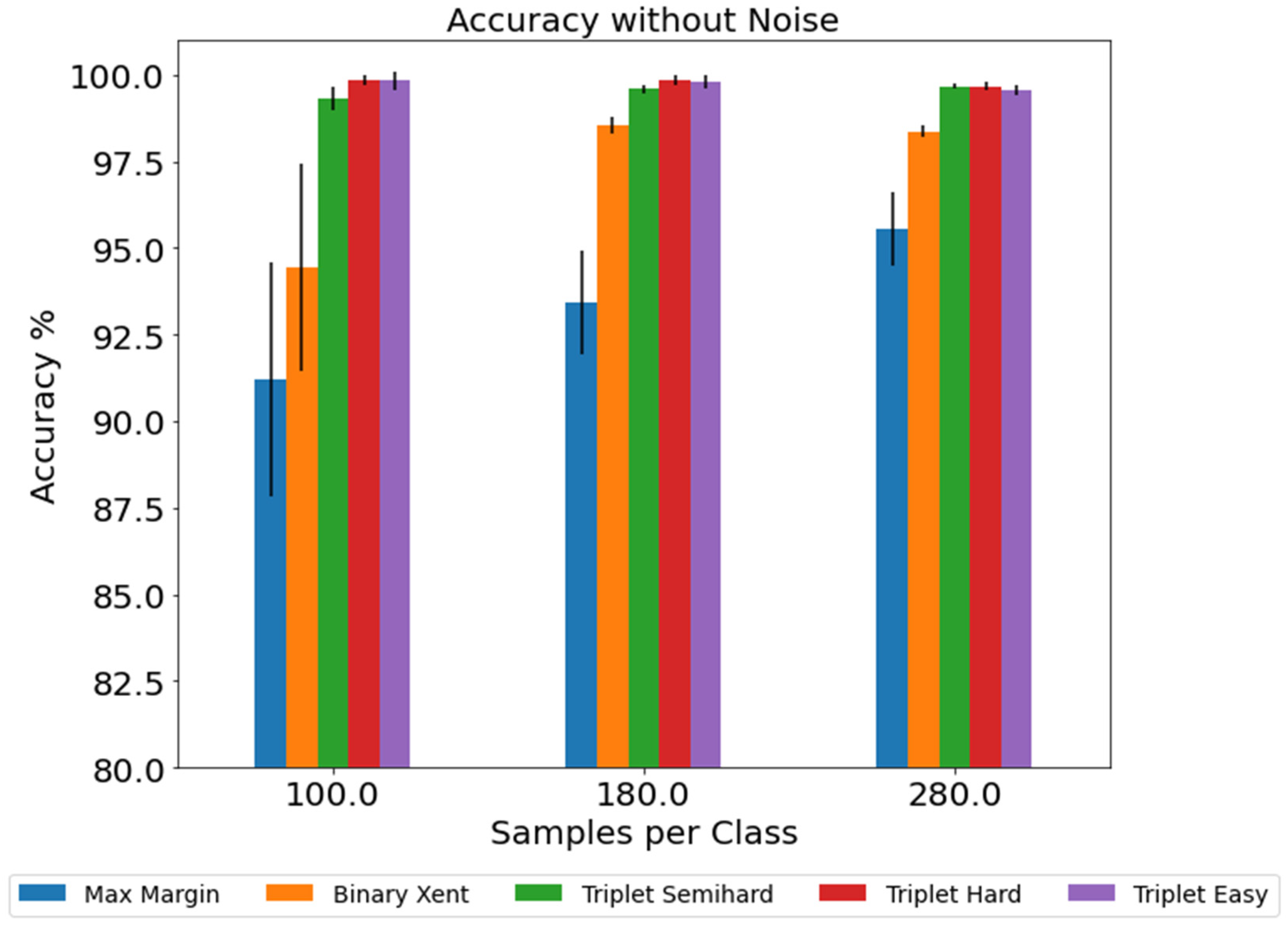
3.1. Model Performance According to The Number of Training Samples

The five models were evaluated using different numbers of training samples to simulate the lack of training data observed in real-world stamping process scenarios. Each class was evaluated according to three sample sets, namely 100, 180, and 280 (all data) samples. These sets were then divided into training and test sets containing 60% and 40% of the samples, respectively. Each class sample set was randomly sampled five times, and each random sample was trained and tested four times. In total, every class sample set underwent 20 training processes, each of which generated a new model. This procedure was intended to mitigate randomness. The procedure is illustrated in Figure 9.

Figure 10 presents the results of each loss function performance. The x-axis of Figure 10 represents the total number of samples for the training and test sets. One-shot ten-way testing was conducted to evaluate the test set. As illustrated in Figure 10, the triplet loss function yielded the most favorable results, with greater than 99% accuracy for the hard, semihard, and hard-soft-margin batches. The binary cross-entropy loss function yielded the second-best results, in which accuracy increased concurrently with an increasing number of training samples. The contrastive max-margin function yielded the least favorable results, with 95.56% accuracy when training was conducted with all available samples.

Figure 10 also presents the standard deviation for each calculation; the triplet loss function yielded the highest accuracy and exhibited the lowest standard deviation, the value of which decreased concurrently with increase in the number of training samples. All loss functions exhibited high standard deviations when trained using the lowest number of training samples, with the contrastive max-margin and binary cross-entropy functions exhibiting the highest testing accuracy.

To determine the efficacy of each loss function to enable each feature extractor (FE) to distinguish between different classes, embedding projections were produced for every FE (Figure 11).

Each model was trained and tested using all available samples, and the results supported the previous results presented in Figure 10. Compared with untrained FEs, all models trained using loss functions exhibited some degree of improvement, but the results varied somewhat. In particular, the max-margin loss function provided the least distinguished groupings for each class in comparison with the other loss functions; that is, the class groupings appeared scattered. In addition, the max-margin loss function was the least accurate when trained and tested with all available samples (Figure 10). However, the binary cross-entropy loss function provided much greater embedding compared to that provided by the max-margin loss function. The binary cross-entropy loss function provided the distinguished embedding values required to group the samples, exhibiting a 2.81% increase in accuracy compared with that of the max-margin loss function. The triplet loss function exhibited the most favorable results, with small variations in accuracy among the different batch strategies.

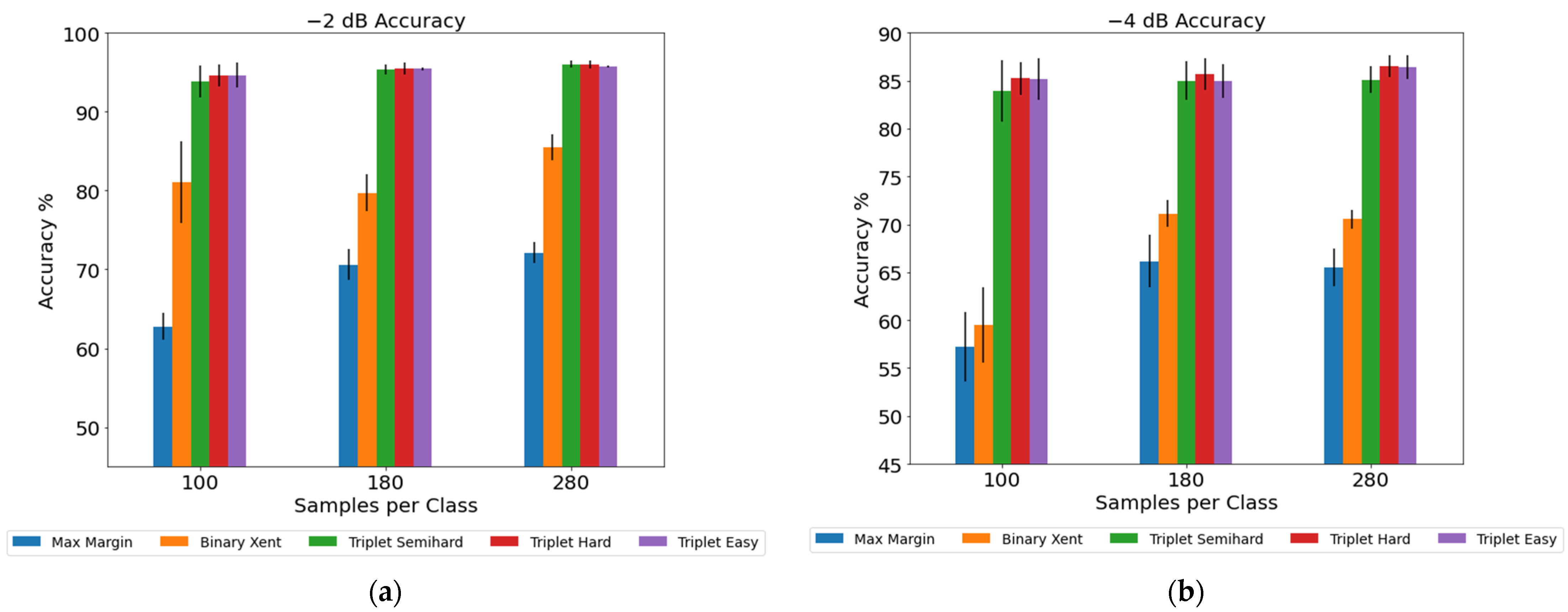
3.2. Model Performance under Noised Test Samples

In this experiment, we evaluated the robustness of each method to the ever-changing conditions of mechanical environments by adding Gaussian noise to the test sets. The signal-to-noise ratio (21) measures the power ratio of a signal compared with the noise applied to the signal, and in our case, we applied a noise power higher than the signal power (−2 dB and −4 dB, respectively) to simulate an environment with high-noise conditions.

$$SN{R}_{dB}=10{\log }_{10}\left(P_{signal}/P_{noise}\right)$$

(21)

As we did in the previous experiment, we used 100, 180, and 280 (all data) samples per class for the training and test sets (Figure 12).

The results (Figure 13) indicate the accuracy of each loss function. In general, for all loss functions, the accuracy increased, and the standard deviation decreased when the number of training samples increased. The triplet loss function exhibited the most favorable result for the −2 dB (Figure 13a) signal-to-noise ratio, with the semihard, hard, and hard-soft-margin batch strategies achieving accuracies of 96.0%, 95.94%, and 95.75% for the highest number of training samples and 93.86%, 94.60%, and 94.64% for the lowest number of training samples, respectively.

The binary cross-entropy function did not exhibit an increase in accuracy when tested using 100 and 180 samples per class for the training and test sets, but it did exhibit a high standard deviation with the lowest number of training set samples per class, even though it achieved higher accuracy than the 80 samples per class (81.03% for 60 samples) set, indicating that the model had low precision. The max-margin loss function achieved the lowest accuracy (72.14%), even with highest number of training set samples per class. However, with the lowest number of training set samples per class (60 and 180), it did not exhibit a high standard deviation, despite the FEM not being able extract the most meaningful features.

The triplet loss function exhibited a drop in accuracy of 9–10% for the −4 dB signal-to-noise ratio test set compared with its accuracy in the −2 dB signal-to-noise ratio test set (Figure 13a). The binary cross-entropy loss function exhibited a high standard deviation in accuracy when it was trained with 60 samples per class, but its accuracy dropped to 57.21%. The max-margin loss function yielded the lowest accuracy compared with the accuracies of the other loss functions, and in terms of the low signal-to-noise ratio (−4 dB), it exhibited a high standard deviation in accuracy when tested 20 times for each training set.

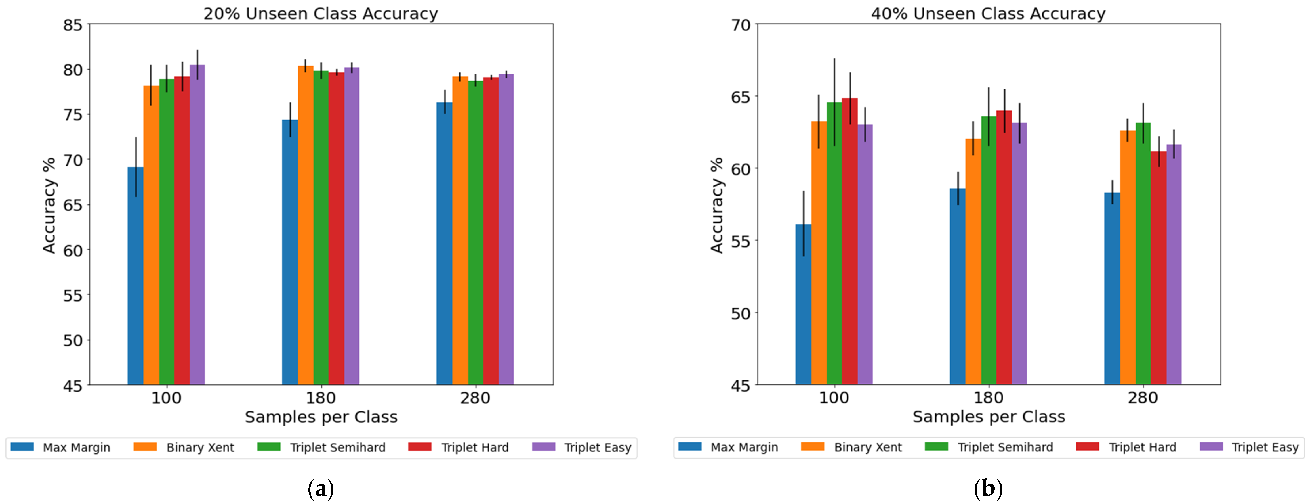
3.3. Performance under New Classes

In this experiment, we evaluated a simulated scenario in which a new class could be recognized by the model without the need for model retraining. We evaluated all loss functions by using the test set combined with unseen classes to be identified by the model during training. The unseen classes were randomly chosen, and the percentages of unseen classes in the test sets were 20% and 40% of the total number of samples in each set, respectively. Additionally, no noise was added to the training or test sets, as illustrated in Figure 14.

Notably, when minibatches were generated for the samples in the test sets, the unseen class was used as an anchor and employed for the target samples. Essentially, the model compared more than 20% and 40% of seen and unseen samples per test set, respectively.

The results (Figure 15a) revealed the accuracy of each loss function tested using the 20% unseen class test set. The triplet loss and binary cross-entropy functions achieved similar accuracies, 80.44% and 80.31%, respectively. However, these accuracies were achieved with 60 and 108 training samples per class, not 168 samples. We suspect that the model was able to generalize the training samples, but was not fully able to recognize the unseen class. In addition, even when it was trained with a higher number of training samples, the FE still was unable to learn essential features; the high number of samples in the test class resulted in low accuracy for 280 samples per class because the model had to recognize more unseen classes. For the test set with 40% (Figure 15b) unseen classes, the FE exhibited a lower ability to extract meaningful features when tested with a high number of test samples; moreover, even though the standard deviation decreased with increases in the number of training samples, the accuracy also decreased.

4. Conclusions

This study presents a stamping tool condition diagnosis method based on DML. Several DML methods were compared to determine which one was the most suitable for stamping tool condition diagnosis. The probability method employs binary cross-entropy, the contrastive method employs contrastive max-margin loss, and the triplet network method employs three batch-generation strategies (semihard, hard, and easy). The main contributions of this study are as follows. First, we compared methods incorporating several types of evaluations. Second, we evaluated the methods by using various numbers of training samples, and the results revealed that the triplet network was the most accurate, followed by the probability and the contrastive methods. Third, we evaluated the methods by using a noise test data set, and for this experiment, the triplet network also demonstrated the most favorable results, followed by the probability and contrastive methods. Finally, we evaluated each method in terms of its ability to recognize new classes. The triplet and probability methods, which achieved similar results, exhibited the best performance, followed by the contrastive method.

In general, the triplet network provided the most favorable results overall, and was most suitable for stamping tool condition diagnosis. However, when subjected to new classes, triplet networks may not be able to provide sufficient accuracy when used with the number of data samples employed in the present study. This problem may be mitigated with additional data.

References

1. American Industrial Metal Stamping Continues to Grow in 2019–2020. Available online: http://www.americanindust.com/blog/metal-stamping-continues-to-grow-2019-2020/ (accessed on 25 January 2021).
2. Ambhore, N.; Kamble, D.; Chinchanikar, S.; Wayal, V. Tool Condition Monitoring System: A Review. Mater. Today Proc. 2015, 2, 3419–3428. [Google Scholar] [CrossRef]
3. Ge, M.; Du, R.; Xu, Y. Hidden Markov Model Based Fault Diagnosis for Stamping Processes. Mech. Syst. Signal Process. 2004. [Google Scholar] [CrossRef]
4. Bassiuny, A.M.; Li, X.; Du, R. Fault Diagnosis of Stamping Process Based on Empirical Mode Decomposition and Learning Vector Quantization. Int. J. Mach. Tools Manuf. 2007, 47, 2298–2306. [Google Scholar] [CrossRef]
5. Ubhayaratne, I.; Pereira, M.P.; Xiang, Y.; Rolfe, B.F. Audio Signal Analysis for Tool Wear Monitoring in Sheet Metal Stamping. Mech. Syst. Signal Process. 2017, 85, 809–826. [Google Scholar] [CrossRef]
6. Shanbhag, V.V.; Rolfe, B.F.; Pereira, M.P. Investigation of Galling Wear Using Acoustic Emission Frequency Characteristics. Lubricants 2020, 8, 25. [Google Scholar] [CrossRef] [Green Version]
7. Shanbhag, V.V.; Pereira, P.M.; Rolfe, F.B.; Arunachalam, N. Time Series Analysis of Tool Wear in Sheet Metal Stamping Using Acoustic Emission. J. Phys. Conf. Ser. 2017, 896, 012030. [Google Scholar] [CrossRef] [Green Version]
8. Sari, D.Y.; Wu, T.L.; Lin, B.T. Study of Sound Signal for Online Monitoring in the Micro-Piercing Process. Int. J. Adv. Manuf. Technol. 2018, 97, 697–710. [Google Scholar] [CrossRef]
9. Ge, M.; Du, R.; Zhang, G.; Xu, Y. Fault Diagnosis Using Support Vector Machine with an Application in Sheet Metal Stamping Operations. Mech. Syst. Signal Process. 2004, 18, 143–159. [Google Scholar] [CrossRef]
10. Zhang, G.; Li, C.; Zhou, H.; Wagner, T. Punching Process Monitoring Using Wavelet Transform Based Feature Extraction and Semi-Supervised Clustering. Procedia Manuf. 2018, 26, 1204–1212. [Google Scholar] [CrossRef]
11. Zhou, C.; Zhang, W. A New Process Monitoring Method Based on Waveform Signal by Using Recurrence Plot. Entropy 2015, 17, 6379–6396. [Google Scholar] [CrossRef] [Green Version]
12. Sah, S.; Gao, R.X. Process Monitoring in Stamping Operations through Tooling Integrated Sensing. J. Manuf. Syst. 2008, 27, 123–129. [Google Scholar] [CrossRef]
13. Zhao, R.; Yan, R.; Chen, Z.; Mao, K.; Wang, P.; Gao, R.X. Deep Learning and Its Applications to Machine Health Monitoring. Mech. Syst. Signal Process. 2019, 115, 213–237. [Google Scholar] [CrossRef]
14. Wen, L.; Li, X.; Gao, L.; Zhang, Y. A New Convolutional Neural Network-Based Data-Driven Fault Diagnosis Method. IEEE Trans. Ind. Electron. 2018, 65, 5990–5998. [Google Scholar] [CrossRef]
15. Zhang, J.; Sun, Y.; Guo, L.; Gao, H.; Hong, X.; Song, H. A New Bearing Fault Diagnosis Method Based on Modified Convolutional Neural Networks. Chin. J. Aeronaut. 2020, 33, 439–447. [Google Scholar] [CrossRef]
16. Wu, J. Sensor Data-Driven Bearing Fault Diagnosis Based on Deep Convolutional Neural Networks and s-Transform. Sensors 2019, 19, 2750. [Google Scholar] [CrossRef] [Green Version]
17. Eren, L.; Ince, T.; Kiranyaz, S. A Generic Intelligent Bearing Fault Diagnosis System Using Compact Adaptive 1D CNN Classifier. J. Signal Process. Syst. 2019, 91, 179–189. [Google Scholar] [CrossRef]
18. Eren, L. Bearing Fault Detection by One-Dimensional Convolutional Neural Networks. Math. Probl. Eng. 2017, 2017, 8617315. [Google Scholar] [CrossRef] [Green Version]
19. Wang, Y.; Yang, H.; Yuan, X.; Shardt, Y.A.W.; Yang, C.; Gui, W. Deep Learning for Fault-Relevant Feature Extraction and Fault Classification with Stacked Supervised Auto-Encoder. J. Process Control 2020, 92, 79–89. [Google Scholar] [CrossRef]
20. Zhang, Y.; Li, X.; Gao, L.; Chen, W.; Li, P. Ensemble Deep Contractive Auto-Encoders for Intelligent Fault Diagnosis of Machines under Noisy Environment. Knowl. Based Syst. 2020, 196, 105764. [Google Scholar] [CrossRef]
21. Zhao, X.; Jia, M.; Liu, Z. Semisupervised Deep Sparse Auto-Encoder With Local and Nonlocal Information for Intelligent Fault Diagnosis of Rotating Machinery. IEEE Trans. Instrum. Meas. 2021, 70, 1–13. [Google Scholar] [CrossRef]
22. Mallak, A.; Fathi, M. Sensor and Component Fault Detection and Diagnosis for Hydraulic Machinery Integrating LSTM Autoencoder Detector and Diagnostic Classifiers. Sensors 2021, 21, 433. [Google Scholar] [CrossRef]
23. Sun, W.; Shao, S.; Zhao, R.; Yan, R.; Zhang, X.; Chen, X. A Sparse Auto-Encoder-Based Deep Neural Network Approach for Induction Motor Faults Classification. Measurement 2016, 89, 171–178. [Google Scholar] [CrossRef]
24. Liu, C.; Zhu, L. A Two-Stage Approach for Predicting the Remaining Useful Life of Tools Using Bidirectional Long Short-Term Memory. Measurement 2020, 164, 108029. [Google Scholar] [CrossRef]
25. Liang, J.; Wang, L.; Wu, J.; Liu, Z.; Yu, G. Elimination of End Effects in LMD by Bi-LSTM Regression Network and Applications for Rolling Element Bearings Characteristic Extraction under Different Loading Conditions. Digit. Signal Process. 2020, 107, 102881. [Google Scholar] [CrossRef]
26. Jalayer, M.; Orsenigo, C.; Vercellis, C. Fault Detection and Diagnosis for Rotating Machinery: A Model Based on Convolutional LSTM, Fast Fourier and Continuous Wavelet Transforms. Comput. Ind. 2021, 125, 103378. [Google Scholar] [CrossRef]
27. Ma, M.; Mao, Z. Deep-Convolution-Based LSTM Network for Remaining Useful Life Prediction. IEEE Trans. Ind. Inform. 2021, 17, 1658–1667. [Google Scholar] [CrossRef]
28. Zhao, R.; Yan, R.; Wang, J.; Mao, K. Learning to Monitor Machine Health with Convolutional Bi-Directional LSTM Networks. Sensors 2017, 17, 273. [Google Scholar] [CrossRef] [PubMed]
29. Huang, C.-Y.; Dzulfikri, Z. Stamping Monitoring by Using an Adaptive 1D Convolutional Neural Network. Sensors 2021, 21, 262. [Google Scholar] [CrossRef]
30. Bromley, J.; Guyon, I.; LeCun, Y.; Säckinger, E.; Shah, R. Signature Verification Using a “Siamese” Time Delay Neural Network. In Proceedings of the 6th International Conference on Neural Information Processing Systems, Virtual-Only, 6–12 December 2020; Available online: https://dl.acm.org/doi/10.5555/2987189.2987282 (accessed on 24 July 2021).
31. Ahmed, S.; Basher, A.; Reza, A.N.R.; Jung, H.Y. A Brief Overview of Deep Metric Learning Methods; Korea Next Generation Computing Society: Jeju, Korea, 2018; Volume 4, p. 5. [Google Scholar]
32. Kaya, M.; Bilge, H.Ş. Deep Metric Learning: A Survey. Symmetry 2019, 11, 1066. [Google Scholar] [CrossRef] [Green Version]
33. Hadsell, R.; Chopra, S.; LeCun, Y. Dimensionality Reduction by Learning an Invariant Mapping. In Proceedings of the 2006 IEEE Computer Society Conference on Computer Vision and Pattern Recognition (CVPR’06), New York, NY, USA, 17–22 June 2006. [Google Scholar]
34. Schroff, F.; Kalenichenko, D.; Philbin, J. FaceNet: A Unified Embedding for Face Recognition and Clustering. In Proceedings of the 2015 IEEE Conference on Computer Vision and Pattern Recognition (CVPR), Boston, MA, USA, 7–12 June 2015. [Google Scholar]
35. Li, X.; Zhang, W.; Ding, Q. A Robust Intelligent Fault Diagnosis Method for Rolling Element Bearings Based on Deep Distance Metric Learning. Neurocomputing 2018, 310, 77–95. [Google Scholar] [CrossRef]
36. Wang, S.; Wang, D.; Kong, D.; Wang, J.; Li, W.; Zhou, S. Few-Shot Rolling Bearing Fault Diagnosis with Metric-Based Meta Learning. Sensors 2020, 20, 6437. [Google Scholar] [CrossRef]
37. Zhang, A.; Li, S.; Cui, Y.; Yang, W.; Dong, R.; Hu, J. Limited Data Rolling Bearing Fault Diagnosis with Few-Shot Learning. IEEE Access 2019, 7, 110895–110904. [Google Scholar] [CrossRef]
38. Liu, J.; Gibson, S.J.; Mills, J.; Osadchy, M. Dynamic Spectrum Matching with One-Shot Learning. Chemom. Intell. Lab. Syst. 2019, 184, 175–181. [Google Scholar] [CrossRef]
39. Weinberger, K.Q.; Blitzer, J.; Saul, L.K. Distance Metric Learning for Large Margin Nearest Neighbor Classification. J. Mach. Learn. Res. 2009, 10, 207–244. [Google Scholar]
40. Hermans, A.; Beyer, L.; Leibe, B. In Defense of the Triplet Loss for Person Re-Identification. arXiv Preprint 2017, arXiv:1703.07737. [Google Scholar]
Figure 1. Siamese neural network architecture.
Applsci 11 06959 g001
Figure 2. Triplet network architecture.
Applsci 11 06959 g002
Figure 3. The goal of triplet learning.
Applsci 11 06959 g003
Figure 4. Easy, hard and semihard triplet illustration, a represent represents an anchor sample and p represents a positive sample; a hard triplet selects a negative in the hard triplet region; a semihard triplet selects a negative sample in semihard (α) region, and an easy triplet selects a negative sample in easy region.
Applsci 11 06959 g004
Figure 5. Monitored locations of the tool die.
Applsci 11 06959 g005
Figure 6. Data transformation from time based to frequency based.
Applsci 11 06959 g006
Figure 7. Sequential 1D CNN architecture.
Applsci 11 06959 g007
Figure 8. Model Configurations.
Applsci 11 06959 g008
Figure 9. Performance evaluation based on various numbers of training samples.
Applsci 11 06959 g009
Figure 10. Accuracy of each model relative to the number of training and testing samples.
Applsci 11 06959 g010
Figure 11. Comparison of principal component analysis (PCA) from embedding projections for all trained FEMs and untrained FEM.
Applsci 11 06959 g011
Figure 12. Performance evaluation based on various numbers of training samples and added noise on test data.
Applsci 11 06959 g012
Figure 13. Accuracy of the max-margin, binary cross-entropy, and triplet semihard, hard, and hard-soft-margins when tested with the −2 dB (a); and −4 dB (b) signal-to-noise ratio noise test sets.
Applsci 11 06959 g013
Figure 14. Performance evaluation based on various numbers of training samples over the unseen class.
Applsci 11 06959 g014
Figure 15. Accuracy of max-margin, binary cross-entropy, and triplet semihard, hard, and hard-soft-margin with test sets containing 20% (a) and 40% (b) unseen classes.
Applsci 11 06959 g015