A Particle PHD Filter for Dynamic Grid Map Building towards Indoor Environment

Abstract

The PHD (Probability Hypothesis Density) filter is a sub-optimal multi-target Bayesian filter based on a random finite set, which is widely used in the tracking and estimation of dynamic objects in outdoor environments. Compared with the outdoor environment, the indoor environment space and the shape of dynamic objects are relatively small, which puts forward higher requirements on the estimation accuracy and response speed of the filter. This paper proposes a method for fast and high-precision estimation of the dynamic objects’ velocity for mobile robots in an indoor environment. First, the indoor environment is represented as a dynamic grid map, and the state of dynamic objects is represented by its grid cells state as random finite sets. The estimation of dynamic objects’ speed information is realized by using the measurement-driven particle-based PHD filter. Second, we bound the dynamic grid map to the robot coordinate system and derived the update equation of the state of the particles with the movement of the robot. At the same time, in order to improve the perception accuracy and speed of the filter for dynamic targets, the CS (Current Statistical) motion model is added to the CV (Constant Velocity) motion model, and interactive resampling is performed to achieve the combination of the advantages of the two. Finally, in the Gazebo simulation environment based on ROS (Robot Operating System), the speed estimation and accuracy analysis of the square and cylindrical dynamic objects were carried out respectively when the robot was stationary and in motion. The results show that the proposed method has a great improvement in effect compared with the existing methods.

1. Introduction

At present, with more and more robots entering our life, how to make robots have the ability of safe and fast dynamic obstacle avoidance has become a hot topic of mobile robot research. In the classical robot obstacle avoidance algorithm, which introduces the relative velocity information of a robot and dynamic object, better obstacle avoidance effect can be obtained [1,2,3], but how to quickly and accurately obtain the dynamic object is a very important challenge. For example, because of the randomness of human motion and the limited indoor space, it is difficult to track and estimate it quickly.

In the field of general target tracking, the random finite set (RFS) theory [4,5,6] provides a mathematical and rigorous method for multi-objective Bayesian state estimation, which can cover all the situations that the standard Bayes filter cannot, including multiple appearing/disappearing objects, imperfect detection, and non-standard measurements. After the random finite set was first proposed by Mahler [4,5], several classical Bayes filters were designed and developed based on this theory. However, the filter directly estimates the posterior probability density of multiple targets based on random finite sets, which involves set integrals and is difficult to be solved analytically. In the most general setting, these random finite set-based stochastic filters can be implemented only using the sequential Monte Carlo method [7,8], or using approximations methods such as the Probability Hypothesis Density (PHD) filter [9,10,11], the Cardinalized PHD filter [12,13], and the Labeled Multi-Bernoulli filter [14,15]. The Probability Hypothesis Density (PHD) filter, which approximates the full multi-object density using the first-order statistical moment of the RFS known as the intensity function or the PHD, is developed to alleviate the computational intractability. The PHD filter operates on the single-target state space and greatly simplifies the calculation problems. At same time, this advantage accelerates the application of random finite set theory in multi-target estimation problems.

In the field of robot and autopilot, it is very important to get the position and speed of the object around it. Several approaches have been presented to combine grid mapping and multi-object tracking toward automatic driving. The classical occupancy grid maps divide the whole environment into independent grid cells and calculate the probability of occupancy of each grid separately. The classic occupancy grid maps are widely used in SLAM (simultaneous location and mapping) and are an important tool for path planning and obstacle collision avoidance for their explicit free-space estimate and ability to represent arbitrarily shaped objects. Danescu et al. [16,17] proposed using particles to characterize the dynamic state of a grid cell, which greatly reduces the amount of calculation to estimate the state of the grid. In order to improve the utilization of particles, Negre et al. [18] and Tanzmeister et al. [19] proposed that particles only characterize the grid occupied cells by dynamic objects instead of all the occupied grid cells. However, they did not give a stochastically rigorous definition of a multi-object state estimation problem.

Theoretically, any dynamic environment can be represented as a random finite set consisting of several point targets (corresponding to grid cells). Therefore, it is intuitively believed that the combination of PHD filter and grid map for multi-target tracking can achieve good results. However, PHD filter has two basic assumptions: one is that each target can only produce one measurement, and the other is that the alarm measurements conform to Poisson distribution. When using grid maps to represent the measurement model, one object will affect the whole area and make an intensity contribution to each cell. At the same time, there are fixed measurements at every moment equal to the number of all grids. However, the PHD filter is based on the framework of RFS, the number of elements in an RFS should be random, and the clutter should satisfy Poisson distribution. The paper [20] proposed limiting the response of the target in only one resolution cell in the image observation and set a threshold value for the measurements to make it meet the two basic requirements of PHD filter. On the basis of [20], the paper [21] analyzed the problem of overestimating the number of targets theoretically and proposed a clustering method to solve the problem of overestimating the number of targets instead of limiting the response of target in one cell. However, they all assume that the physical size of the object is less than the resolution cell. For example, setting the grid size to 1 m is obviously not suitable for an indoor navigation environment.

Steyer et al. [22] proposed an object tracking method based on a dynamic grid map. This method utilizes the feedback from these object tracks to the cell-level representation, and then the occupied grid cell can be individually associated with the object tracks without the need to use clustering methods for the objects that have been tracked. The object track is modeled as an oriented rectangular box. When calculating the size and reference position of the rectangular box, not only the relevant occupancy grid cells is considered, but also the measured free space evidence adjacent to each object box is considered, making the estimation more robust and accurate. In the paper [23], the dynamic object is represented as a modified occupancy grid map. Unlike traditional occupancy grid representation, the modified grid map is only used to keep track of the grids that may be occupied at the next moment. Then, GM-PHD is used to track the grid map, which can complete the tracking and shape estimation of multiple dynamically extended objects. This method can achieve a 20% improvement in the OSPA metric error compared to the baseline GM-PHD filter.

Nuss et al. [24,25] proposed combining MIB filters on the basis of PHD filters (PHD/MIB filter) and gave a strict mathematical definition for the building of dynamic grid maps based on random finite set (RFS) theory. This algorithm uses parallel acceleration to build dynamic grid maps in real time. However, multi-target estimation based on PHD/MIB filter uses a fixed number of particles to resample, which makes the efficiency very low. Since the new particle generation method is based on the Bernoulli filter method in each grid (under DS evidence theory, the mass value is greater than zero) and the constant velocity model is used, the system has a poor estimation effect on the maneuvering target and when the target just enters the field of view.

In summary, the combination of PHD filter and grid map for dynamic object estimation shows promising results. However, they usually set the range of the dynamic grid map to a fixed size, which is very inflexible and cannot gradually expand the sensing range with the movement of the robot. At the same time, they are mainly aimed at outdoor environments. For indoor environments, due to the small space, filters are required to estimate the state of dynamic objects with faster speed and accuracy.

The main contributions of this article are as follows: First, 2D Lidar is used to estimate the state of dynamic objects in indoor environments and the dynamic environment is represented by a dynamic grid map, which simplifies the problem of data association between measurements and targets in the PHD filter. The dynamic grid map is bound to the robot coordinate system, so that the size of the dynamic grid map remains unchanged with the movement of the robot, and the update equation of the particle state with the movement of the robot is deduced. Second, the CV and CS motion models are fused, which improves the system’s perception speed and accuracy of maneuvering objects and reduces the fluctuations in the estimation of constant-velocity moving objects. Third, a simulation environment was built in Gazebo, and a program was developed based on the ROS (Robot Operating System) environment and GPU parallel computing to verify the effectiveness of the algorithm.

The rest of the paper is organized as follows. In Section 2, we describe the preliminaries for a PHD filter-based random finite set and the particle realization of PHD filter under a grid map. In Section 3, the implementation details of building dynamic grid maps for indoor environments are presented. Some simulations are carried out in Section 4, and the conclusions are given in Section 5.

2. Particle Realization of PHD Filter under Grid Map

2.1. Multi-Object Bayesian Filter and PHD Filter Based on Random Finite Set

Suppose that there are $n_k$ target objects and $m_k$ observations in the environment at time $k$, which are represented as $\{x_k^{(1)},\dots ,x_k^{(n_k)}\}$ and $\{z_k^{(1)},\dots ,z_k^{(m_k)}\}$, respectively. The number of objects and the state of each object are random variables; then, the state of multiple targets of the environment at time $k$ can be represented as a random finite set $X_k=\{x_k^{(1)},\cdots ,x_k^{(n_k)}\}\in F(\varsigma )$, where $x_k^{(n_k)}\in \varsigma$ and $\mathsf{\Psi }(\varsigma )$ is the finite subset of $\varsigma$. Similarly, the multi-target observations can be expressed by random finite sets $Z_k=\{z_k^{(1)},\dots ,z_k^{(m_k)}\}\in \mathsf{\Psi }({\rm Z})$, where $z_k^{(m_k)}\in Z$ and $\mathsf{\Psi }(Z)$ is the finite subset of $Z$.

The multi-objective Bayesian filter directly estimates the posterior probability density of multi-objective at $k+1$ time through the observation until the time $k+1$ [26,27]. The iterative process of the algorithm can be divided into a prediction and update process. Assuming that the posterior probability density of multi-objective is ${\pi }_k(X_k|{\mathrm{Z}}_{1:k})$ at time $k$, the predicted posterior probability density of multi-objective is:

$${\pi }_{k+1|k}(X_{k+1}|{\mathrm{Z}}_{1:k})={\displaystyle \int f_{k+1|k}(X_{k+1}|X_k){\pi }_k(X_k|{\mathrm{Z}}_{1:k})\delta X_k}$$

(1)

where $f_{+}(X_{k+1}|X_k)$ represents the multi-target transfer density, which can be approximated by the motion model of the object. When the observation $Z_{k+1}$ is received at time $k+1$, the updating equation of multi-target posterior probability density is as follows:

$${\pi }_{k+1|k+1}(X_{k+1}|{\mathrm{Z}}_{1:k+1})=\frac{{\psi }_k(X_{k+1}|Z_{k+1}){\pi }_{k+1|k}(X_{k+1}|{\mathrm{Z}}_{1:k+1})}{{\displaystyle \int {\psi }_{k+1}(X_{k+1}|Z_k){\pi }_{k+1|k}(X_{k+1}|{\mathrm{Z}}_{1:k+1})\delta X_{k+1}}}.$$

(2)

The integral over multi-object probability density function is set integral as:

$${\displaystyle \int f(X)}\delta X=f(\varnothing )+{\displaystyle \sum _{i=1}^{\infty }\frac{1}{n!}}{\displaystyle \int f(x_1,\cdots x_n)}d{x}_1\cdots d{x}_n.$$

(3)

The number of objects is also a variable that makes integration difficult at the same time. So, it can only be used to estimate the limit number of targets and usually adopts SMC (Sequential Monte Carlo) methods [7,28]. In order to overcome this difficulty, Mahler proposed PHD filter [10,11,29], which operates directly on the first-order statistical moment, greatly simplifying the calculation. The standard PHD filter modeling process includes the prediction:

$$D_{k+1|k}(x|z_{1:k})={\gamma }_{k+1}(x)+{\displaystyle \int (e_{k+1|k}(x_k)}{f}_{k+1|k}(x|x_k)+b_{k+1|k}(x|x_k))D_k(x_k|z_{1:k})d{x}_k$$

(4)

and update equation:

$$\begin{array}{l}{D}_{k+1|k+1}(x|z_{1:k+1})=(1-p_D(x))D_{k+1|k}(x)+\\ \hspace{0.17em}\hspace{0.17em}\hspace{0.17em}\hspace{0.17em}\hspace{0.17em}\hspace{0.17em}\hspace{0.17em}\hspace{0.17em}\hspace{0.17em}\hspace{0.17em}\hspace{0.17em}\hspace{0.17em}\hspace{0.17em}\hspace{0.17em}\hspace{0.17em}\hspace{0.17em}\hspace{0.17em}\hspace{0.17em}\hspace{0.17em}\hspace{0.17em}\hspace{0.17em}\hspace{0.17em}\hspace{0.17em}\hspace{0.17em}{\displaystyle \sum _{z\in Z_{k+1}}\frac{p_{D }(x)g_{k+1}(z|x_{k+1|k}^r)D_{k+1|k}(x)}{{\kappa }_{k+1}(z)+{\displaystyle \int p_D(\zeta )g_{k+1}(z|\zeta )D_{k+1|k}(\zeta )d\zeta }}}\end{array}$$

(5)

where $b_{k+1|k}(x_{k+1}|x_k)$ denotes the PHD of RFS $B_{k+1|k}(x_k)$ spawned by a target with previous state $x_k$ and ${\gamma }_{k+1}(x_{k+1})$ denotes the PHD of the spontaneous birth RFS ${\mathsf{\Gamma }}_{k+1}$ at time $k+1$.$f_{k+1|k}(\cdot |\cdot )$ denotes the transition probability density of individual targets.${\kappa }_{k+1}(z)={\lambda }_{k+1}c(z)$ is the intensity of false alarms, ${\lambda }_{k+1}$ is the average number of Poisson clutter points per scan, $c(z)$ denotes clutter probability density. $Z_{k+1}=\{z_{k+1}^{(1)},\dots ,z_{k+1}^{(n_{k+1})}\}\in \mathsf{\Psi }({\rm Z})$ is the time-sequence of observation sets, $z$ is one of the measurements in $z_{k+1}^{(n_{k+1})}$, $p_D(x)$ is the state dependent probability of detection, and $g_{k+1}(z|x_{k+1|k}^r)$ is the likelihood of individual targets. Since the PHD propagation equations involve multiple objects integrals that have no computationally tractable closed-form expression, the sequential Monte Carlo (SMC) methods are used to approximate the PHD [28]. This paper selects particle methods to realize PHD filter on the dynamic grid map.

2.2. Measurement-Driven Particle PHD Filter Realization Based on Grid Map

Let the PHD $D_{k|k}(x|z_{1:k})$ at time $k$ be represented by a set of $\upsilon$ particles and its weights ${\{x_k^i,w_k^i\}}_{i=1}^{\upsilon }$:

$$D_{k|k}(x|z_{1:k})\approx {\displaystyle \sum _{i=1}^{\upsilon }{w}_{k|k}^i{\delta }_{x_{k|k}^i}(x)}.$$

(6)

Here, ${\delta }_a(x)$ is the Dirac delta function, which centers in $a$. The predicted particles include persistent particles and newborn particles, which are generated by:

$$x_{k+1|k}^i~\{\begin{array}{l}{q}_{k+1}(•|x_k^i)\\ b_{k+1}(•|Z_{k+1})\end{array}.$$

(7)

The $q_{k+1}(•|x_k^i)$ and $b_{k+1}(•|Z_{k+1})$ are the proposal density of the surviving particles and the newborn particles, respectively. Usually, suppose that the proposal density $q_{k+1}(•|x_k^i)$ is equal to the transition density $f_{+}(x_{k+1}|x_k)$. The sampling provides the two sets of particles, persistent particle set ${\{x_{k+1|k,p+}^i,w_{k+1|k,p+}^i\}}_{i=1}^{L_p}$ and newborn particle set ${\{x_{k+1|k,b}^i,w_{k+1|k,b}^i\}}_{i=1}^{L_b}$ where persistence particle weights are multiplied with the persistence probability $w_{k+1|k,p+}^i=p_S{w}_{k|k,p}^i$ and newborn particle weights are all equal to a constant system preset value. Due to the randomness of the newborn particles, it is often beneficial to consider their influence on the state estimation only after another recursion. So, the predicted PHD should be represented by the persistent set [9,30]:

$$D_{k+1|k}(x|z_{1:k+1})={\displaystyle \sum _{i=1}^{L_p}{w}_{k+1|k,p+}^i{\delta }_{x_{k+1|k,p+}^i}(x)}.$$

(8)

The standard PHD update can be represented as:

$$\begin{array}{l}{D}_{k+1|k+1}(x|z_{1:k+1})={\displaystyle \sum _{r=1}^L{w}_{k+1|k+1}^r\delta (x-x_{k+1|k+1}^r)}\\ w_{k+1|k+1}^r={\displaystyle \sum _{z\in Z}\frac{g_k(z|x_{k+1|k}^r)w_{k+1|k}^r}{{\kappa }_{k+1}(z)+{\displaystyle \sum _{j=1}^L{g}_{k+1}(z|x_{k+1|k}^j)w_{k+1|k}^j}}}\end{array}.$$

(9)

In this paper, the observation is provided by the measurement grid map (with $n\times m$ resolution cells) calculated through every laser scan. The observations can be represented at time step $k$ by $z_k=\{z_k^{i,j}:i=1,\cdots ,n,j=1,\cdots ,m\}$ and all observations up to $k$ can be represented by $Z_{1:k}=\{z_t:t=1,\cdots ,k\}$. Then, the particle weight update equation can be transformed into [31]:

$$w_{k+1|k+1}^r=\frac{{\displaystyle \prod _{i\in C_i(x_{k+1|k}^r)}{\displaystyle \prod _{j\in C_j(x_{k+1|k}^r)}g(z_k^{i,j}|x_{k+1|k}^r)}}}{K_k(z)+C_k(z_k^{r,s})}{w}_{k+1|k}^r$$

(10)

where $g(z_k^{i,j}|x_{k+1|k}^r)$ is the importance weight, which can be calculated by using the likelihood ratio in cell $(i,j)$ for a target in state $x_{k+1|k}^r$. $C_i(x_{k+1|k}^r)$ and $C_j(x_{k+1|k}^r)$ are the sets of subscripts i and j, indicating the neighboring regions affected by the targets. $K_k(z)$ is a normalization constant to represent the clutter density. Meanwhile, $C_k(z_k^{r,s})$ is given by:

$$C_k(z_k^{r,s})={\displaystyle \sum _{p\in P^{r,s}}{\displaystyle \prod _{i\in C_i(x_{k+1|k}^r)}{\displaystyle \prod _{j\in C_j(x_{k+1|k}^r)}g(z_k^{i,j}|x_{k+1|k}^r)}}{w}_{k+1|k}^r}.$$

(11)

After the particle weights are updated, we can resample the new particle set ${\{x_{k+1|k+1,p}^i,w_{k+1|k+1,p}^i\}}_{i=1}^v$ from the persistent particle set ${\{x_{k+1|k,p+}^i,w_{k+1|k+1,p+}^i\}}_{i=1}^{L_p}$ and the newborn particle set ${\{x_{k+1|k,b}^i,w_{k+1|k+1,b}^i\}}_{i=1}^{L_b}$ according to their weight. Where $v=M_{p}M$, $w_{k+1|k+1,p}^i=\frac{1}{v}({\displaystyle \sum _{i=1}^{L_p}{w}_{k+1|k+1,p+}^i}+{\displaystyle \sum _{i=1}^{L_b}{w}_{k+1|k+1,b}^i})$. PHD RFS of multi-target at time $k+1$ can be represented by:

$$D_{k+1|k}(x|z_{1:k+1})={\displaystyle \sum _{i=1}^v{w}_{k+1|k+1,p}^i{\delta }_{x_{k+1|k+1,p}^i}(x)}.$$

(12)

3. The Proposed Framework for Building Dynamic Grid Map

The system framework of the whole design is shown in Figure 1. The 2D Lidar is used as a sensor to perceive the dynamic environment, and the particle PHD filter is used to estimate the velocity of dynamic objects. The system is based on the ROS framework and uses GPU to perform parallel acceleration calculations. The details of the implementation process are as follows.

3.1. Preprocessing of LIDAR Measurements

In order to improve the obstacle avoidance ability of the robot, the real-time performance of a dynamic grid map must be guaranteed. However, in the process of building a dynamic grid map with a particle-based PHD filter, it often needs a large number of particles to achieve better estimation of objects, and more particles will reduce the real-time performance of the system, which also limits the number of particles. However, there are many static objects (such as walls, tables) in the indoor navigation environment. Similar environments are established in Gazebo, as shown in Figure 2a. The white object represents the robot, the yellow object represents a moving dynamic object, and the rest are static objects. The prior map and laser measurements are shown in Figure 2b, and red indicates the laser measurements. If all the scanning points measured by the laser are input into the particle filter for estimation, the particles distribution of the filter is shown in Figure 2c. It can be found that a large number of particles are occupied on the static walls and tables for the estimation of zero velocity. In the same number of particles, this will reduce the state estimation effect of yellow dynamic objects. However, the static object information can be directly transmitted to the global planner through the static cost map during navigation, and it does not need to estimate the speed information. Therefore, in order to use as few particles as possible to estimate the dynamic object better, the input filter measurements must be preprocessed first.

In order to solve this problem, firstly, a prior grid map is used to preprocess to get an inflated occupancy probability grid map. Assuming that the grid coordinate is $(inde{x}_x^i,inde{y}_x^i)$, the nearest distance from the obstacle is $dis$, and then the occupancy probability function of the grid cell is:

$$M((inde{x}_x^i,inde{y}_x^i))=\{\begin{array}{l}{e}^{-\frac{di{s}^2}{2{\sigma }^2}} dis<dis\_th\\ 0 else\end{array}$$

(13)

where $dis$ is the nearest distance from the grid cell to the obstacle in the prior map, $dis\_th$ is the distance threshold for calculating occupancy probability, and $\sigma$ is the set constant parameter. Using the depth-first method, we can calculate the occupancy probability of the entire grid map from the grid cell occupied by obstacles. Since the inflated occupancy probability grid map only needs to be calculated once, the real-time performance of the system will not be reduced.

According to the robot position $(x_{map}^r,y_{map}^r,thet{a}_{map}^r)$, the laser point coordinates in the Lidar coordinate system can be projected into the map coordinate system to obtain its occupancy probability and judge whether it is a dynamic object or static object. For the $i\_th$ laser point, we can directly obtain the polar measurements $ranges\left[i\right]$ and $angles\left[i\right]$ in the Lidar coordinate system, so the Cartesian coordinates in the Lidar coordinate system can be obtained:

$$\{\begin{array}{l}{x}_{laser}^i=ranges[i]\ast \cos (theatas[i])\\ y_{laser}^i=ranges[i]\ast \sin (theatas[i])\end{array}.$$

(14)

Then, the coordinates $(x_{map}^i,y_{map}^i)$ of the $i\_th$ laser point in the coordinates of the world coordinate system (map) can be calculated (assuming that the robot coordinate system coincides with the Lidar coordinate system):

$$\{\begin{array}{l}{x}_{map}^i=x_{map}^r+x_{laser}^i\ast \cos (thet{a}_{map}^r)-y_{laser}^i\ast \sin (thet{a}_{map}^r)\\ y_{map}^i=y_{map}^r+x_{laser}^i\ast \sin (thet{a}_{map}^r)+y_{laser}^i\ast \cos (thet{a}_{map}^r)\end{array}.$$

(15)

Assuming that the origin of the grid map is $(x_{map}^{org},y_{map}^{org})$ and the grid size is $reso$, then the grid coordinates of the $i\_th$ laser point are

$$S_i=((x_{map}^i-x_{map}^{org})/reso,(y_{map}^i-y_{map}^{org})/reso).$$

(16)

According to the grid cell coordinates $S_i$, the corresponding occupancy probability $M(S_i)$ can be obtained by indexing the occupancy probability grid map calculated above. When the occupancy probability is larger than a threshold, it means that the $i\_th$ laser point falls on the original static object, and it does not need to be input into the particle-based PHD filter to estimate its velocity; otherwise, it needs to be input. The test environment established in Gazebo is shown in Figure 3a and the yellow area shown in Figure 3b is the inflated occupation grid map obtained by expanding on the prior grid map. After the static laser points are removed, the particles distribution estimated by filter is shown in Figure 3c.

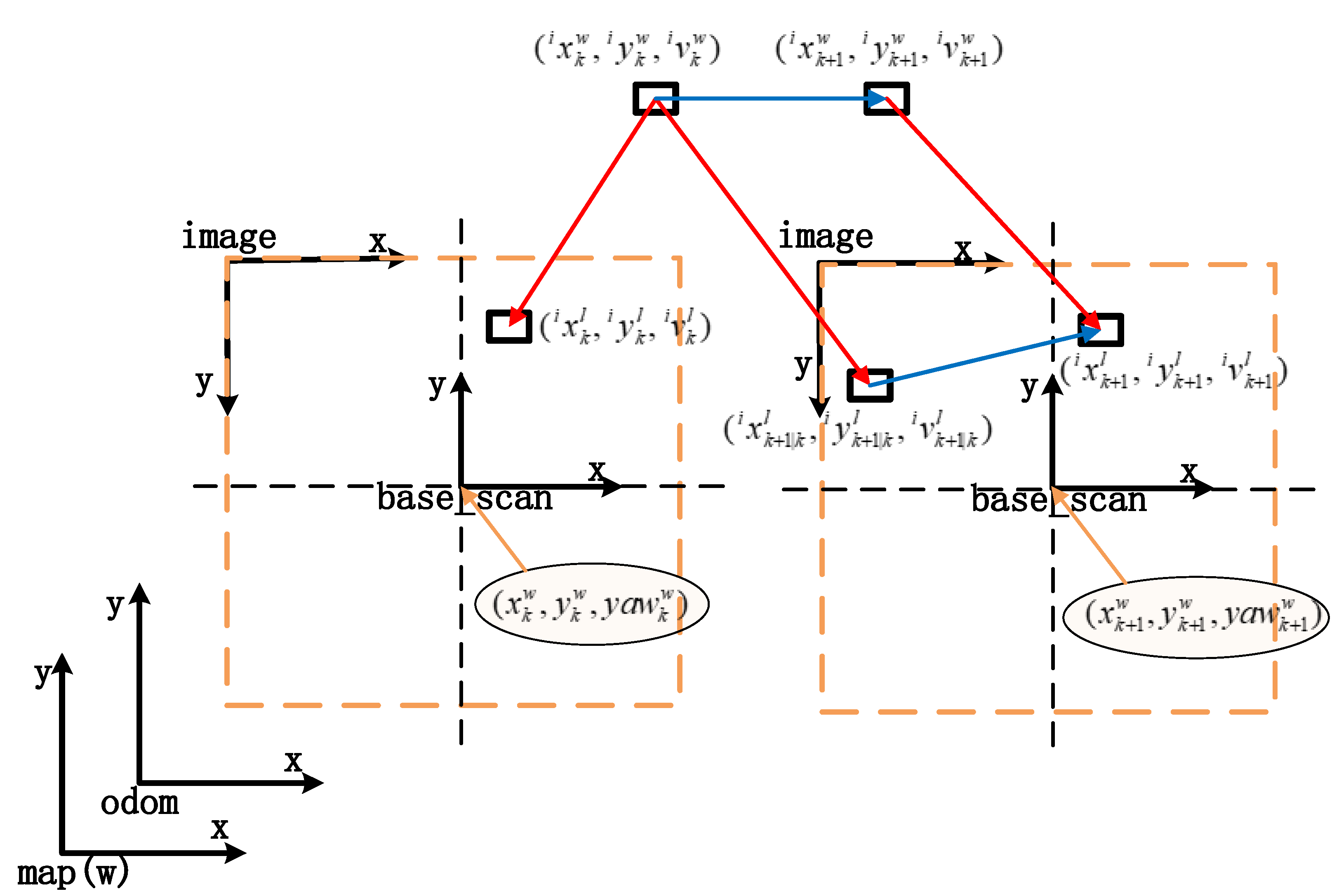
3.2. Particle State Updating with Robot Motion

One of the factors that affects the computing speed of the particle-based PHD filter is the number of grid cells $N_{grid\_cells}$. Suppose that the length and width of the dynamic grid map are $ma{p}_{size\_x}$, $ma{p}_{size\_y}$, and the grid cell size is $reso$; then: $N_{grid\_cells}=\frac{ma{p}_{size\_x}·ma{p}_{size\_y}}{reso·reso}$. The size and the speed range of moving objects (such as people) in indoor environments are smaller than those of outdoor moving objects (airplanes and cars). In order to accurately describe the shape and speed of objects, a smaller resolution is needed. At the same time, in order to ensure the running speed of the system, the size of the dynamic map must be appropriate. Therefore, the local dynamic grid map attached to the robot is used for estimation instead of global dynamic grid map estimation, and then, the global velocity of the dynamic object is calculated using the robot’s pose. Supposing that the positions of the robot at time $k$ and $k+1$ are $(x_k^w,y_k^w,ya{w}_k^w)$, $(x_{k+1}^w,y_{k+1}^w,ya{w}_{k+1}^w)$, the particle states are $({}^{i}x_k^l,{}^{i}y_k^l,{}^{i}v_k^l)$, $({}^{i}x_{k+1}^l,{}^{i}y_{k+1}^l,{}^{i}v_{k+1}^l)$, and the state of the object in the corresponding world coordinate system is $({}^{i}x_k^w,{}^{i}y_k^w,{}^{i}v_k^w)$, $({}^{i}x_{k+1}^w,{}^{i}y_{k+1}^w,{}^{i}v_{k+1}^w)$, where $i\in (1,N)$ is the number of particles, as shown in Figure 4 below.

As shown in Figure 4, we transform the particle state at time $k$ to the state at time $k+1$ as:

$$R_k\ast {}^{i}X_k^l+t_k=R_{k+1}\ast {}^{i}X_{k+1|k}^l+t_{k+1}={}^{i}X_k^w.$$

(17)

Meanwhile:

$$R_{k+1}\ast {}^{i}X_{k+1}^l+t_{k+1}={}^{i}X_{k+1}^w.$$

(18)

From Equations (17) and (18), we can obtain:

$${}^{i}X_{k+1}^w-{}^{i}X_k^w=R_{k+1}({}^{i}X_{k+1}^l-{}^{i}X_{k+1|k}^l)$$

(19)

and

$${}^{i}X_{k+1|k}^l=R_{k+1}^{-1}(R_k\ast {}^{i}X_k^l+t_k-t_{k+1}).$$

(20)

Dividing both sides by the time interval $dt$ between two frames at the same time, it is considered that a dynamic object moves uniformly in the world coordinate system when $dt$ is small. Then, Equation (19) can be transformed into a speed expression form:

$$v_k^w=R_k{v}_k^l=v_{k+1|k}^w=R_{k+1}{v}_{k+1|k}^l$$

(21)

and

$$v_{k+1|k}^l=R_{k+1}^{-1}{R}_k{v}_k^l.$$

(22)

From the above, we can find that by converting the information of particles at the time $k$ into the time $k+1$ according to Equations (20) and (22), we can complete the estimation from the local dynamic grid map to the global dynamic grid map. The details of the implementation process are as follows.

• Obtaining the position of robot

• The transformation from the base_scan (robot) coordinate system to the odom coordinate system can be obtained through the odometry topic published by Gazebo or using TF_Listener, and the transformation of the odom and map coordinate system can be predefined in a roslaunch file in a simulation environment. In the actual positioning process, the pose of the robot can be obtained by slam positioning or Monte Carlo positioning in navigation.

2.

Update of particle position information

• The scale coordinates of the $i\_th$ particle in a local dynamic grid map system of time $k$ are $({}^{i}x_k^l\ast reso,{}^{i}y_k^l\ast reso)$.
• The scale translational coordinates of the base_scan coordinate system relative to the local dynamic grid map coordinate system are $(ma{p}_{size\_x}/2\ast reso,ma{p}_{size\_y}/2\ast reso)$.
• The scale coordinates of the $i\_th$ particle in the base_scan coordinate system of time $k$ are $({}^{i}x_k^l-ma{p}_{size\_x}/2,ma{p}_{size\_y}/2-{}^{i}y_k^l)\ast reso$.
• Coordinates of the $i\_th$ particle in the world system:

  $${\left[\begin{array}{l}x\\ y\end{array}\right]}_w=\left[\begin{array}{cc}\cos (ya{w}_k^w)& -\sin (ya{w}_k^w)\\ \sin (ya{w}_k^w)& \cos (ya{w}_k^w)\end{array}\right]\left[\begin{array}{l}({}^{i}x_k^l-ma{p}_{size\_x}/2)\ast reso\\ (ma{p}_{size\_y}/2-{}^{i}y_k^l)\ast reso\end{array}\right]+\left[\begin{array}{l}{x}_k^w\\ y_k^w\end{array}\right].$$

  (23)
• Coordinate transformation from the world coordinate system to the $k+1$ coordinate system:

  $$\left[\begin{array}{l}({}^{i}x_{k+1|k}^l-ma{p}_{size\_x}/2)\ast reso\\ (ma{p}_{size\_y}/2-{}^{i}y_{k+1|k}^l)\ast reso\end{array}\right]=\left[\begin{array}{cc}\cos (ya{w}_{k+1}^w)& -\sin (-ya{w}_{k+1}^w)\\ \sin (-ya{w}_{k+1}^w)& \cos (ya{w}_{k+1}^w)\end{array}\right]({\left[\begin{array}{l}x\\ y\end{array}\right]}_w-{\left[\begin{array}{l}{x}_{k+1}^w\\ y_{k+1}^w\end{array}\right]}_w).$$

  (24)

3.

Update of particles velocity

• Assume that the $i\_th$ particle velocities at time $k$ in the dynamic grid map coordinate system are ${}^{i}v_k^l=({}^i\dot{x}_k^l,{}^i\dot{y}_k^l)$.
• The $i\_th$ particle velocities at time $k+1$ in the base coordinate system are

  $$\begin{array}{l}\left[\begin{array}{l}{}^i\dot{x}_{k+1|k}^l\\ {}^i\dot{y}_{k+1|k}^l\end{array}\right]=\left[\begin{array}{cc}\cos (yaw\_diff)& -\sin (yaw\_diff)\\ \sin (yaw\_diff)& \cos (yaw\_diff)\end{array}\right]\left[\begin{array}{l}{}^i\dot{x}_k^l\\ -{}^i\dot{y}_k^l\end{array}\right]\\ yaw\_diff= ya{w}_{k+1}^w-ya{w}_k^w\end{array}.$$

  (25)
• When converting the velocity $\left[\begin{array}{l}{}^i\dot{x}_{k+1|k}^l\\ {}^i\dot{y}_{k+1|k}^l\end{array}\right]$ of the $i\_th$ particle to the local dynamic grid coordinate system of time $k+1$, we need to multiply ${}^i\dot{y}_{k+1|k}^l$ by minus one.

3.3. Motion Model Design

Considering the space limit of the indoor environment, the speed of the system to estimate the dynamic object must be improved. Dynamic objects not only exist in a state of constant velocity but also in a state of acceleration, deceleration, and turning. The CS (Current Statistical) model has a better performance when tracking maneuvering objects, but when it estimates uniform motion, the error has a large fluctuation. Here, we combine the two to improve its estimation effect in maneuvering and uniform motion. The standard CS model for two-dimensional motion is:

$$X_{k+1|k}={\varphi }_{k+1|k}{X}_k+U_k{\overline{a}}_k+w(k)$$

(26)

where $x_k=[x_k,y_k,{\dot{x}}_k,{\dot{y}}_k,{\ddot{x}}_k,{\ddot{y}}_k]$ is a vector that includes position, velocity, and acceleration information and ${\overline{a}}_k=[{\overline{a}}_x,{\overline{a}}_y]$ is the mean acceleration of the dynamic object. The specific matrices expression of ${\varphi }_{k+1|k}$ and $U_{k+1|k}$ can be shown as follows:

$$\begin{array}{l}{\varphi }_{k+1|k}=\left[\begin{array}{cccccc}1& 0& \Delta t& 0& {\phi }_1& 0\\ 0& 1& 0& \Delta t& 0& {\phi }_1\\ 0& 0& 1& 0& {\phi }_2& 0\\ 0& 0& 0& 1& 0& {\phi }_2\\ 0& 0& 0& 0& {\phi }_3& 0\\ 0& 0& 0& 0& 0& {\phi }_3\end{array}\right]\\ U_{k+1|k}={\left[\begin{array}{cccccc}{u}_1& 0& u_2& 0& u_3& 0\\ 0& u_1& 0& u_2& 0& u_3\end{array}\right]}^T\end{array}$$

(27)

where:

$$\begin{array}{l}{\phi }_1=(\tau \Delta t-1+e^{-\tau \Delta t})/{\tau }^2\\ {\phi }_2=(1-e^{-\tau \Delta t})/\tau \\ {\phi }_2=e^{-\tau \Delta t}\\ u_1=(-\tau \Delta t+{(\tau \Delta t)}^2/2+1-e^{-\tau \Delta t})/{\tau }^2\\ u_2=(\tau \Delta t-1+e^{-\tau \Delta t})/\tau \\ u_2=1-e^{-\tau \Delta t}\end{array}$$

(28)

where $\tau$ is the reciprocal of the acceleration time constant and $\Delta t$ is the time interval between the two samples. The $w(k)$ is Gaussian white noise, and its variance is:

$$Q_k=2\tau {\sigma }_a^{2}q=2\tau {\sigma }_a^2\left[\begin{array}{cccccc}{q}_{11}& 0& q_{12}& 0& q_{13}& 0\\ 0& q_{11}& 0& q_{12}& 0& q_{13}\\ q_{12}& 0& q_{22}& 0& q_{23}& 0\\ 0& q_{12}& 0& q_{22}& 0& q_{23}\\ q_{13}& 0& q_{23}& 0& q_{33}& 0\\ 0& q_{13}& 0& q_{23}& 0& q_{33}\end{array}\right].$$

(29)

The constant matrix $q$ is related to $\Delta t$ and $\tau$, which can be represented as follows:

$$\begin{array}{l}{q}_{11}=(1-e^{-2\tau \Delta t}+2\tau \Delta t+2{(\tau \Delta t)}^3/3-2{(\tau \Delta t)}^2-4\tau \Delta t{e}^{-\tau \Delta t})/(2{\tau }^5)\\ q_{12}=(1+e^{-2\tau \Delta t}-2e^{-\tau \Delta t}+2\tau \Delta t{e}^{-\tau \Delta t}-2\tau \Delta t+{(\tau \Delta t)}^2)/(2{\tau }^4)\\ q_{13}=(1-e^{-2\tau \Delta t}-2\tau \Delta t{e}^{-\tau \Delta t})/(2{\tau }^3)\\ q_{22}=(4e^{-\tau \Delta t}-3-e^{-2\tau \Delta t}+2\tau \Delta t)/(2{\tau }^3)\\ q_{23}=(e^{-2\tau \Delta t}+1-2e^{-\tau \Delta t})/(2{\tau }^2)\\ q_{23}=(1-e^{-2\tau \Delta t})/(2\tau )\end{array}.$$

(30)

Here, when ${\overline{a}}_k$ is zero, the CS model becomes a CV (Constant Velocity) model. In order to reduce the estimation error of the object in a uniform motion, a part of the particles (for example, half of the total number of particles) is set as the CV model in the particle prediction stage. Then, it can achieve a better estimation effect in various motion conditions such as acceleration, deceleration, and uniform motion. At the same time, when using the CV model, the acceleration in its state vector is multiplied by a positive number (less than 1), which can restrain the acceleration and make it more stable in the uniform motion stage. After all particles are predicted by the two motion models, the measurement grid map is used to update the particle weights, and then re-sampling can avoid particle attenuation which, more importantly, can realize the interaction between the two models. Through the state statistics, the current acceleration average value of the dynamic object can be obtained, which is used to update the variance of the current acceleration of the particles:

$${({\sigma }_a^i)}^2=\{\begin{array}{l}(4-\pi ){(a_{\max }-{\overline{a}}_k^i)}^2/\pi ,{\overline{a}}_k^i>0\\ (4-\pi ){(-a_{-\max }+{\overline{a}}_k^i)}^2/\pi ,{\overline{a}}_k^i<0\end{array}$$

(31)

where ${\overline{a}}_k^i$ is the average value of acceleration. The $a_{\max }$ and $a_{-\max }$ are the maximum positive and negative accelerations of the target, respectively.

3.4. Particle Weights Update

Using Equation (10) to update the particle weight is still difficult to operate. Here, we draw on the method of paper [23]. The weight of particles is updated in the unit of a grid cell. Suppose that ${\{x_{p,k+1|k}^{i,c},w_{p,k+1|k}^{i,c}\}}_{i=1:N_{p,k+1|k}^c}$ represents the predicted particle set of the grid cell $c$ from time $k$ to $k+1$. Then, the PHD of the dynamic point object RFS in the grid cell $c$ can be expressed as:

$$D_{p,k+1|k}(x_{k+1})={\displaystyle \sum _{i=1:N_{p,k+1|k}^c}{w}_{p,k+1|k}^{i,c}\delta (x_{k+1}-x_{p,k+1|k}^{i,c})}.$$

(32)

According to the definition of PHD, the integral of PHD on the grid cell $c$ is equal to its occupation probability, which is

$$D_{p,k+1|k}(x_{k+1})={\displaystyle \sum _{i=1:N_{p,k+1|k}^c}{w}_{p,k+1|k}^{i,c}\delta (x_{k+1}-x_{p,k+1|k}^{i,c})}.$$

(33)

Since the occupancy probability of the grid cannot exceed one, the sum weights of the particle set of a grid cell needs to be reduced accordingly to make the sum of particle weights one or slightly smaller when the sum of particle weights exceeds one. Based on this, the predicted free mass value can be calculated:

$$m_{p,k+1|k}^c(F_{k+1})=\min (\alpha (t)m_k^c(F_k),1-{\displaystyle \sum _{i=1:N_{p,k+1|k}^c}{w}_{p,k+1|k}^{i,c}})$$

(34)

where $\alpha (t)\in [0,1]$ describes the decreasing prediction reliability related to the time interval. Assuming that at time $k+1$, the grid cell $c$ obtains the measured mass value $m_{z_{k+1}}^c(O_{k+1})$ and $m_{k+1}^c(F_{k+1})$ through laser scan. Then, we can use the Dempster–Shafer rule [32] to combine the predicted mass value and the measured mass value to get the updated mass value $m_{k+1}^c(O_{k+1})$ and $m_{k+1}^c(F_{k+1})$. Then, we can use the updated mass value of occupancy $m_{k+1}^c(O_{k+1})$ to update the weight of the predicted particle set ${\{x_{p,k+1|k}^{i,c},w_{p,k+1|k}^{i,c}\}}_{i=1:N_{p,k+1|k}^c}$:

$$w_{p,k+1}^{i,c}={\mu }_A^c{\tilde{w}}_{p,k+1|k}^{i,c}$$

(35)

where ${\mu }_A^c={({\displaystyle \sum _{i=1:N_{p,k+1|k}^c}{\tilde{w}}_{p,k+1|k}^{i,c}})}^{-1}{m}_{k+1}^c(O_{k+1})$. The state of the particles remains unchanged during the update process. After such processing, the sum of the particle weights of the grid cell $c$ is equal to $m_{k+1}^c(O_{k+1})$.

In order to improve the tracking speed of the dynamic target, the newborn particles of the grid cell $c$ are directly generated according to the measurements. Assuming that the measured occupancy probability of grid c is $m_{z_{k+1}}^c(O_{k+1})$, then the number of new particles generated is $N_{b,k+1}^c=M_b{m}_{z_{k+1}}^c(O_{k+1})$, and the sum of the weights of the particle set is $P_b{m}_{z_{k+1}}^c(O_{k+1})$. When $m_{z_{k+1}}^c(O_{k+1})$ is not zero, the weight of each particle is $w_{b,k+1}^{i,c}=P_b/M_b$, and when it is zero, no particles are generated. Finally, the PHD of the dynamic point object RFS of grid $c$ at time $k+1$ can be expressed as:

$$D_{k+1}(x_{k+1})={\displaystyle \sum _{i=1:N_{p,k+1}^c}{w}_{p,k+1|}^{i,c}\delta (x_{k+1}-x_{p,k+1|k}^{i,c})}+{\displaystyle \sum _{i=1:N_{b,k+1}^c}{w}_{b,k+1|}^{i,c}\delta (x_{k+1}-x_{b,k+1}^{i,c})}.$$

(36)

3.5. Dynamic Object Segmentation and State Estimation

Two-dimensional (2D) Lidar can directly obtain the distance information (ranges) and angle information (thetas) to the object. The range and angle difference of the adjacent measurement laser points on the same object should be within a certain threshold; that is, the same object satisfies $abs(ranges[i+1]-ranges[i])<{\Delta }_{range}$ and $abs(thetas[i+1]-thetas[i])<{\Delta }_{theta}$. The ${\Delta }_{range},{\Delta }_{theta}$ are the designed threshold. When traversing $ranges$ and $thetas$ to copy it to $break\_ranges$ and $break\_thetas$, inserting −1 if the continuous condition is not satisfied. Then, the measurements can be divided as shown in Figure 5. Figure 5a is the storage structure of the raw measurements, and Figure 5b is the storage structure after inserting −1 between two consecutive measurements that do not meet the continuity condition.

Then, we calculate the grid coordinates on the dynamic grid map for all the laser points in each part divided by −1, respectively, and get the maximum and minimum grid coordinates. Considering the movement distance of the object in the sampling interval, a rectangle region $\mathsf{\Omega }$ can represent the range of the dynamic object. The rectangle information includes the starting point information $start\_xy$ and the length information $length\_x$, $length\_y$, as shown in Figure 6.

Then, we only need to perform statistical calculations on the grid cells in the green box, as shown above. The motion information of grid cell $c$ includes speed and acceleration information. Taking ${\overline{v}}_x^c$ as an example, the calculation formula is:

$${\overline{v}}_x^c=\frac{1}{{\displaystyle \sum _{i=1:N_{p,k+1}^c}{w}_{p,k+1}^{i,c}}}{\displaystyle \sum _{i=1:N_{p,k+1}^c}{w}_{p,k+1}^{i,c}{v}_{p,k+1}^{i,c}}$$

(37)

where $v_{p,k+1}^{i,c}$ represents the x-direction velocity of the posterior persistent particle $x_{p,k+1}^{i,c}$ in the grid cell $c$, and the other motion information is calculated in the same way.

After calculating the motion information of each grid cell, due to the small physical size of the dynamic objects in the indoor environment, the average motion velocity of the dynamic objects that can be applied to obstacle avoidance algorithms can be further calculated. For example, the calculation method for the velocity of the dynamic object in the region ${\mathsf{\Omega }}_1$ obtained by the above segmentation method is finding the grid cells ${\mathsf{\Omega }}_{occ}$ that satisfies $m_{k+1}^c(O_{k+1})>\min \_occ$ in the rectangular region ${\mathsf{\Omega }}_1$, the number of which is ${\mathsf{\Omega }}_{num}$, and calculating its average velocity as the speed of the dynamic object:

$$\overline{v}=\frac{1}{{\mathsf{\Omega }}_{num}}{\displaystyle \sum _{i\in {\mathsf{\Omega }}_{occ}}{\overline{v}}^i}.$$

(38)

3.6. Parallel Implementation

The calculation of the measurement grid is very time-consuming. For example, the map size is $20m\times 20m$, and the resolution is $0.05m$, so the number of grid cells needed to be calculated is ${\left(20/0.05\right)}^2=160000$. Under the conditions of serial computing, in order to meet the real-time requirements, it is usually necessary to make a trade-off between the map size and the grid resolution. The occupancy grid map is a computing intensive environment characterization scheme. Due to the limited computing resources, users have to choose between map size and grid resolution. In a dynamic environment, especially for the perception of dynamic objects, it is necessary to ensure a sufficient sensing range (map size) and perceptual accuracy (resolution). This will cause a huge computational load because a large number of grid cells need to be calculated. Some researchers have proposed that GPU (Graphics Processing Units) can be used to accelerate the establishment of a traditional static grid map [33,34]. Here, the method of the paper [34] is used to calculate the measurement grid maps in parallel. Each grid cell contains two information $p_{occ}$ and $p_{free}$. Suppose $n$ measurements $(range{s}_{k+1}^{1:n},theta{s}_{k+1}^{1:n})$ are obtained at time $k+1$. When $range{s}_{k+1}^i$ is greater than the sensing range, it is considered infinite. Then, the calculation process can be summarized into two steps.

• Use the GPU to calculate the polar coordinate measurement grid map in parallel. Assuming that the grid $c_{j,i}$ in the polar coordinate system corresponds to the laser measurement $(range{s}_{k+1}^i,theta{s}_{k+1}^i)$, the inverse sensor model can be used to calculate the occupancy probability of the grid cell $c_{j,i}$:

  $$p_{occ}(c_{j,i}|range{s}_{k+1}^i)=\frac{\alpha (range{s}_{k+1}^i)}{\sqrt{2\pi {\sigma }^2}}{e}^{-\frac{{(c_{j,i}-range{s}_{k+1}^i)}^2}{2}}.$$

  (39)

  At the same time, it is also necessary to use measurement $range{s}_{k+1}^i$ to estimate the free mass value $p_{free}(c_{j,i}|range{s}_{k+1}^i)$ of grid cell $c_{j,i}$. For its calculation, please refer to the paper [26].
• After calculating the measurement grid map in polar coordinates, it needs to be converted into the measurement grid map in Cartesian coordinates. Here, the polar coordinate grid needs to be correctly mapped to the grid under Cartesian coordinates, and the value in the grid can be interpolated correctly. Here, it is necessary to correctly map the grid cell in polar coordinates to the corresponding grid cell in Cartesian coordinates and correctly interpolate $p_{occ}$ and $p_{free}$ in the grid cell. In the paper, different conversion methods are compared, including the exact algorithm and the sampling approach. Here, we use the better texture mapping method and use the OpenGL library to convert the measurement grid map in the polar coordinate system to the measurement grid map in the Cartesian coordinate system.

In order to ensure the accuracy of dynamic grid map estimation, a large number of particles need to be used. At the same time, operations on each particle are involved in the particle prediction phase, update phase, grid statistical moment calculation, and resampling phase. Due to the characteristics of particle filter, these operations can be accelerated through parallel computing [35,36]. After the particle prediction step is performed using the parallel method, since the update of the particle weight and the calculation of the statistical moment are all based on the grid cell, each grid cell must record the particles in the grid cell. Here, we first sort the particles according to their grid coordinates. After sorting the particles, each grid cell only needs to store two particle subscripts: the first subscript and the last subscript of all particles in this grid cell. The sorted particles will be traversed in parallel and when the grid coordinates of the $i\_th$ particle are not equal to the grid coordinates of the $(i-1)\_th$ particle, then the $i\_th$ particle is the first particle of the corresponding grid cell. Similarly, when the grid coordinates corresponding to the $j\_th$ particle and the $(j+1)\_th$ particle are not equal, then the $j\_th$ particle is the last particle of the corresponding grid cell (the first and last particles in the sorted particle set do not need to be judged by this method).

The whole process of sorting and assignment of particles to grid cells is shown in Figure 7. Since the start and last particle corresponding to each grid cell are unique, the association process of particles to grids can be calculated in parallel without GPU memory write conflicts. In the calculation of the statistical moment of each grid cell, it also benefits from the sorting operation of the particles. For the sorted particle set, we can accumulate numerical variable values related to statistical moments in parallel. Then, we can get the statistical moment of the grid cell by traversing each grid in parallel and subtracting the corresponding accumulated value. Therefore, the computational complexity of the statistical moment for each grid cell will no longer depend on the number of particles in the grid cell but rather a fixed value.

4. Simulation

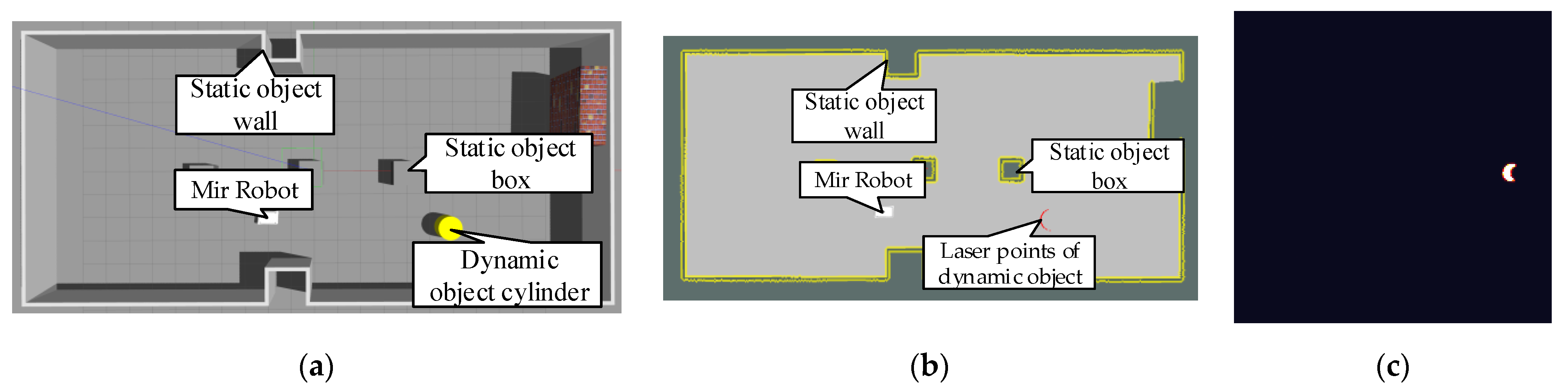
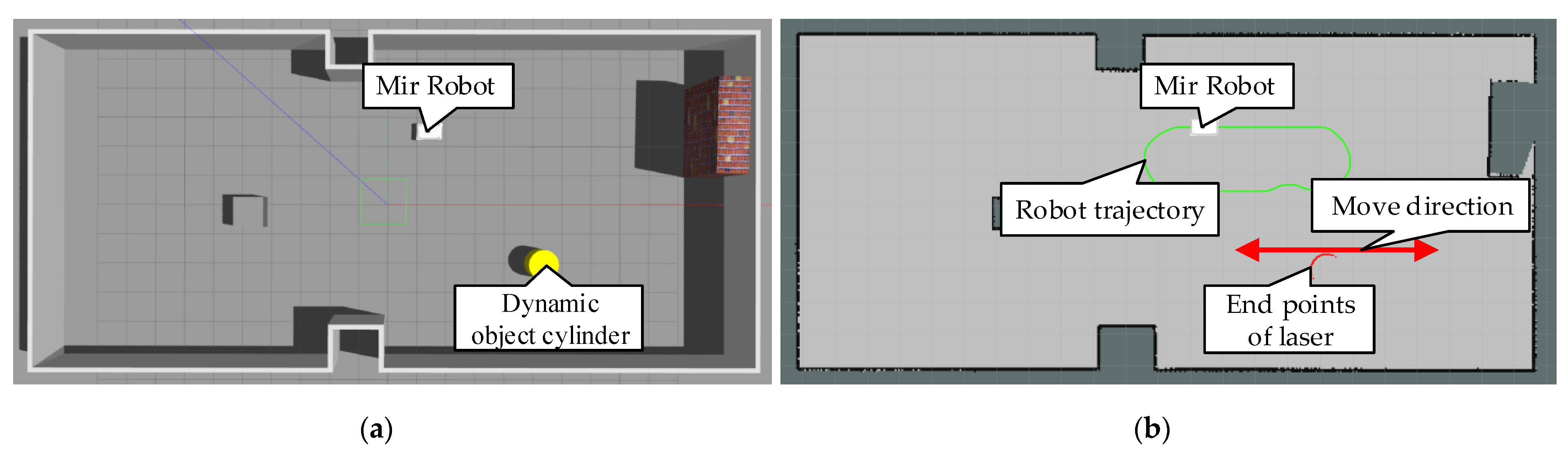
4.1. Simulation Settings

In order to determine whether the dynamic grid map estimate is accurate, we build an environment in Gazebo and load the Mir robot platform, which is equipped with a two-dimensional Lidar directly above it to perceive the surrounding environment. The program is based on the Ubuntu18.04 System and is developed with the help of ROS. The compilation environment is GCC-10.2 and calls the CUDA library to use GPU for parallel acceleration calculations. In order to allow the robot to perceive dynamic objects when the robot and dynamic objects are all in motion, the sensing range of the Lidar needs to be ensured. Here, the scanning range of the Lidar is set to 0–360 degrees, the number of sensing laser points is 1000, the scan cycle 12.5 hz, the size of the dynamic grid map is 20 × 20 square meters, the resolution is 0.05 m, and the other setting parameters of the filter are shown in

Table 1. The filter main parameters.

Parameter	Description	Value
M_p	Persistent number per point	2500
M_b	Birth number per point	500
P_b	Birth probability per point	0.01
$v_b$	Mean velocity of newborn particles	0
${\sigma }_{b,v}$	Variance of newborn particles velocity	30
P_s	Persistence probability	0.95
${\sigma }_p$	Normally distributed variance of noise position	0.1
${\sigma }_v$	Normally distributed variance of noise velocity	2.0
$a_{\max }$	Maximum positive accelerations	25
$a_{-\max }$	Maximum negative accelerations	25

. The simulation experiment is divided into two parts. Section 4.2 is for the situation in which dynamic objects are always moving within the robot’s sensing range, while Section 4.3 is about the situation in which dynamic objects will enter and leave the robot’s sensing area.

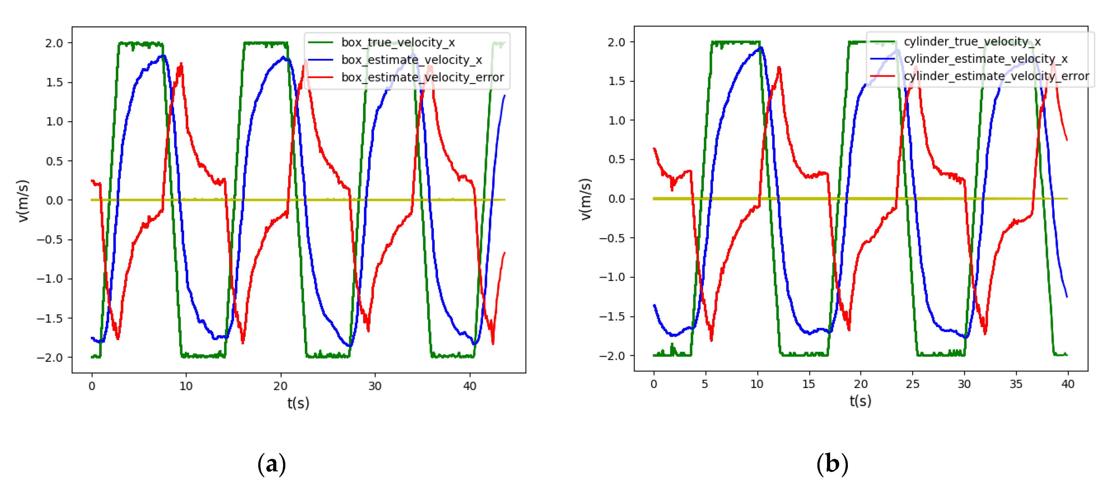
4.2. Accuracy Comparison of Speed Estimation

Aiming at the indoor environment, a typical square object (with a side length of 1 m) and a cylindrical object (with a diameter of 1 m) are selected to estimate their speed under the constant-velocity model and the motion model designed in this paper. The movement of dynamic objects includes acceleration, deceleration, and uniform speed phases.

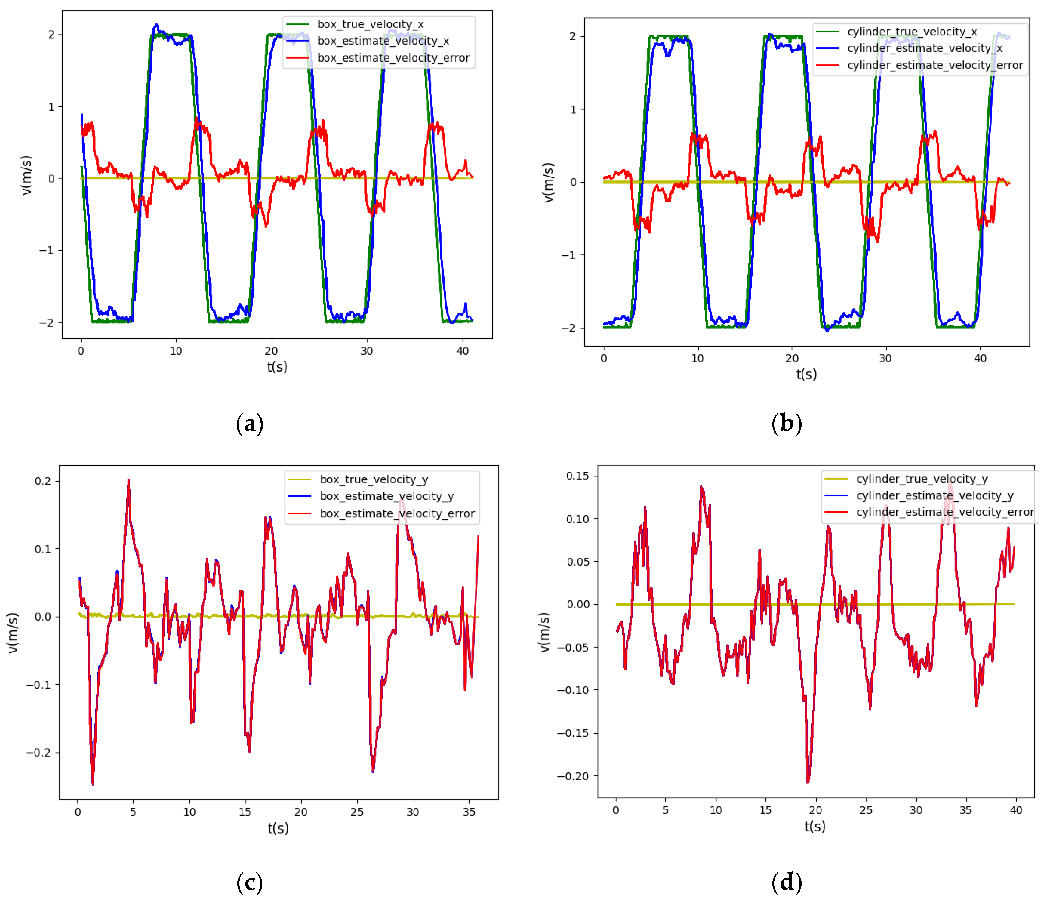
4.2.1. The Robot Is Stationary

In front of the robot, the dynamic object is set (box and cylinder) to reciprocate in the x-direction. The movement process includes acceleration, deceleration, and uniform motion stages. The simulation environment built in Gazebo is shown in Figure 8a. The movement direction of dynamic object is shown in Figure 8b.

Using Equations (37) and (38), we can get the overall average speed of the dynamic object. However, the speed estimated here is based on the grid, which needs to be multiplied by the resolution of the dynamic grid map and converted to metric units. At the same time, it needs to be converted from the speed in the dynamic grid coordinate system to the speed in the global coordinate system using Equation (21). In the ROS environment, by subscribing to the topic of dynamic object status information published by Gazebo, we can directly obtain its true displacement and velocity. The comparison between speed estimation of the filter with the constant-velocity motion model and the true value is shown in Figure 9. Figure 9a is a comparison of the estimated speed with the true value of a box object in the x-direction and Figure 9c is the same comparison in the y-direction. Figure 9b,d are the comparison of the estimated velocity and the true value of the cylinder object in the x and y-directions, respectively.

The speed estimation using the filter with combining the CV and CS motion model proposed in this paper is shown in Figure 10. In order to verify the effectiveness of the algorithm, we use the metric speed error to represent the accuracy of the speed estimation. It can be seen that the absolute value of the speed estimation error of the box object is reduced from more than 1.5 m/s in Figure 9a to less than 0.5 m/s in Figure 10a in the x-direction and the same result is for the cylinder. In the y-direction, the true velocity of the dynamic object is constant zero, and both estimates are relatively accurate. However, in order to improve the estimation effect of the dynamic characteristics of the object, the filter with the proposed motion model introduces acceleration information, which makes the estimation effect worse than that of the filter with using the constant-velocity motion model. Since the measured part of the box and cylinder object did not change significantly when the robot is stationary during the simulation process, the estimation effect of the filter on them does not show an obvious difference.

We evaluate RMSE, Mean Error, and Standard Deviation (S.D.) of the metric absolute speed error in the result. In addition, the improvement values are calculated as shown:

$$\eta =(1-\frac{\beta }{\alpha })\times 100\%$$

(40)

where $\alpha$ is the value of CV motion model, and $\beta$ is the value of the system. The comparison results are shown in

Table 2. The result of the metric absolute speed error when the robot is stationary.

Object		CV Model(m/s)			The System(m/s)			Improvement
		RMSE	MAE	S.D.	RMSE	MAE	S.D.	RMSE	MAE	S.D.
cylinder	x	0.7098	0.5012	0.7069	0.2148	0.1518	0.2052	69.73%	69.71%	70.97%
	y	0.0207	0.0170	0.0205	0.0262	0.0208	0.0263	−26.57%	−22.35%	−28.29%
box	x	0.7029	0.4983	0.7016	0.2036	0.1424	0.2029	71.03%	71.42%	71.08%
	y	0.0142	0.0114	0.0138	0.0179	0.0120	0.0159	−26.05%	−5.26%	−15.27%

. The improvement of the system can reach 70% on average in the main direction x of movement.

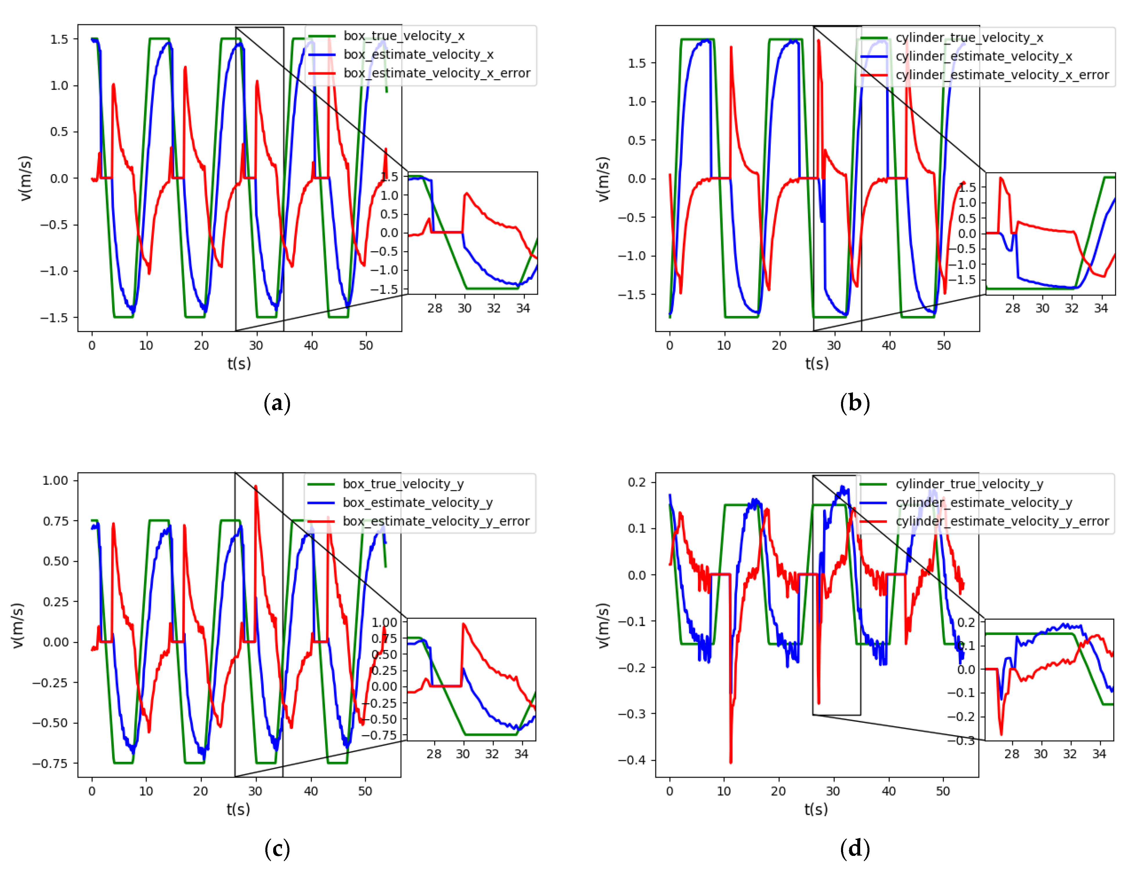
4.2.2. The Robot Is in Motion

We select four target points on the navigation map and use the ROS navigation package to navigate the Mir Robot. The robot reaches the four points in sequence and moves in a loop. The Simulation environment in Gazebo is shown in Figure 11a and the yellow cylinder is the dynamic object to be estimated (a square box object can replace the cylindrical object, and it is not shown in Figure 11a). The robot trajectory is shown as the green line in Figure 11b. The movement of dynamic objects is the same as in Section 4.2.1, and the trajectory is shown by the red arrow.

The comparison result of the speed estimation using the filter with the CV motion model is shown in Figure 12, and combining the CV and CS motion model proposed in this paper is shown in Figure 13 when the Mir Robot is in motion. In the x-direction, the velocity estimation error using the filter with the CV motion model is larger than the estimation error when the robot is stationary, regardless of whether the target is maneuvering or moving at a constant speed. While the filter with the proposed motion model can still achieve a relatively good performance in all motion stages of the dynamic object, although the fluctuation of the estimation speed error has also increased. In the y-direction, the filter’s speed estimation error with the CV motion model or the motion model proposed in this paper both increase significantly and even reach 0.15–0.2 m/s. That is mainly because when the robot and the dynamic object are moving, the area that is not scanned by the laser at the current time may be scanned the next time, and the scanned area may be blocked the next time. As the measurement area of the same object changes, a corresponding speed estimate will be generated, which will eventually be superimposed on the speed estimate of a whole dynamic object, causing the estimation to be biased and the accuracy to decrease.

The comparison of RMSE, Mean Error, and Standard Deviation (S.D.) of the metric absolute speed error when the robot is in motion are shown in

Table 3. The result of the metric absolute speed error when the robot is in motion.

Object		CV Model(m/s)			The System(m/s)			Improvement
		RMSE	MAE	S.D.	RMSE	MAE	S.D.	RMSE	MAE	S.D.
cylinder	x	0.7596	0.6089	0.7218	0.2577	0.2124	0.2576	66.73%	65.71%	64.97%
	y	0.0761	0.0652	0.0727	0.0694	0.0538	0.0667	8.80%	17.48%	8.25%
box	x	0.8210	0.6763	0.8167	0.2910	0.2044	0.2827	64.55%	69.77%	65.38%
	y	0.0774	0.0682	0.0774	0.0856	0.0622	0.0838	−10.59%	8.79%	−8.26%

. Compared with the CV motion model, the proposed method that combines the CS and CV motion model can improve the speed estimation accuracy by more than 65% in the x-direction. In the y-direction, it can be found that the estimation accuracy of the proposed model is close to or even slightly improved compared to the CV motion model. It is further proved that the proposed filter with combining the CS and CV motion model can greatly improve the estimation accuracy and response speed of dynamic objects. At the same time, because the cylindrical measuring part has a smaller change relative to the box measuring part during the simulation process, the speed estimation error in the y-direction is also smaller. This error is difficult to avoid when using the measurement grid map calculated by the current method as the measurement information of the particle filter. The overall average running time of the system is 25 ms including 10 ms for calculating the measurement grid map and 15 ms for filter estimation.

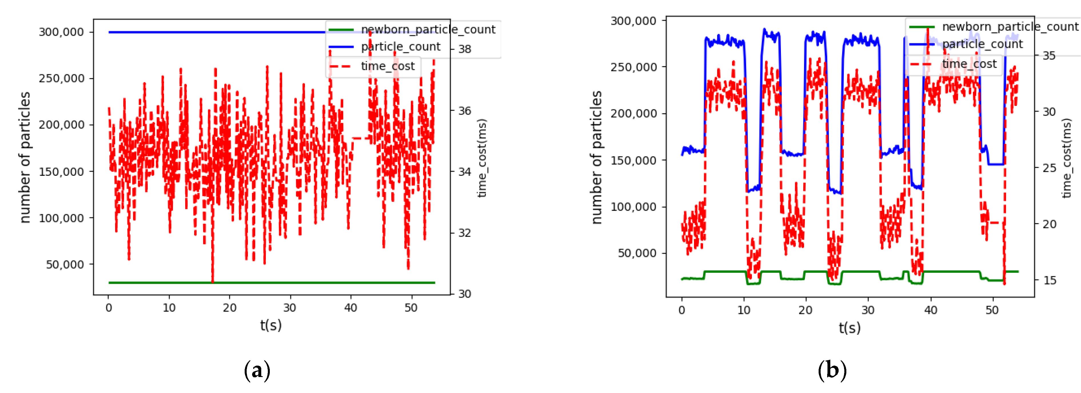
4.3. Speed Estimation of the Dynamic Objects Entering and Leaving the Robot’s Sensing Area

The simulation experiment here is mainly to analyze the performance of the algorithm for estimating the speed of dynamic objects when objects enter and leave the robot’s sensing range. The experimental setup is shown in Figure 14. Figure 14a shows the Gazebo simulation environment, and Figure 14b shows the Rviz interactive interface. The robot’s sensing range is 14 m, and the size of the dynamic grid map is 28 × 28 square meters. The dynamic object moves back and forth in a straight line between the red dots. The blue dotted line is the robot’s sensing range, and the robot is in a static state.

Figure 15 is the speed estimation result in the case of using a fixed number of particles and constant velocity motion model (the method adopted by [16], referred to as the Nuss’s method). In the simulation, the number of newborn particles and persistent particles are fixed to 30,000 and 300,000 respectively. For the disappearance and appearance of dynamic objects, the speed estimation of the algorithm is as shown in the partial zoom figure. When no dynamic objects are detected (disappearing in the robot’s perception range), the speed estimation value and error value are both set to 0. It can be seen from the Figure 15 that the speed estimation curve of Nuss’s method changes relatively smoothly, and it takes a long time to track the true velocity value.

The speed estimation result using the algorithm proposed in this paper is shown in Figure 16, and the simulation parameter settings are the same as Table 1. In the x-movement direction of a dynamic object, since the maximum absolute value of velocity is relatively large (1.5 m/s and 1.8 m/s in the uniform speed stage, respectively), the influence of the small amplitude jitter error is negligible. In the y-direction of motion, the maximum absolute value of the motion velocity is only 0.75 and 0.15, respectively. This small amplitude jitter error will increase the ratio between it and the dynamic object’s own motion velocity, but the overall error value can still be controlled within a relatively small range.

After a dynamic object appears, the maximum absolute value of the algorithm velocity estimation error is regarded as the peak error, and the time taken for the algorithm velocity estimation to stably converge to 90% of the true value is regarded as the convergence time of the algorithm. The comparison results are shown in

Table 4. Algorithm performance comparison.

Dynamic Object	Velocity Direction	Mean of Peak Error (m/s)		Convergence Time(s)
		Nuss’s Method	The Proposed Method	Nuss’s Method	The Proposed Method
box	x-direction	1.1899	0.4654	2.9625	0.312
	y-direction	0.7971	1.0833	3.1125	0.825
cylinder	x-direction	1.7644	1.5356	2.925	0.751
	y-direction	0.2788	0.6005	2.55	1.275

. It can be seen that although the algorithm proposed in this paper has no advantages in terms of peak error, the advantage of this paper is that the convergence time is significantly faster than Nuss’s method, which is very useful for indoor environments with limited space.

The number of newborn particles and persistent particles involved in processing each frame of laser scan data (an algorithm running cycle) and the processing time are shown in Figure 17. It can be seen from the Figure 17b that the number of newborn particles and persistent particles using the algorithm proposed in this paper will change with the number of dynamic objects. When there are few dynamic objects, the calculation load will be greatly reduced. When two dynamic objects appear in the robot’s sensing range at the same time, the computational efficiency of the two methods tends to be close. However, due to the uncertainty of the number of dynamic objects, in order to meet the estimation effect in the case of different numbers of dynamic objects, the Nuss’s method will take a large and fixed number of particles accordingly, resulting in low overall efficiency. In this section, the performance of the algorithm is analyzed and compared when the robot is stationary. For the performance analysis of the algorithm when the robot is in motion, the robot motion setting method in Section 4.2.2 can be used. The conclusion is similar to this section, and it is omitted here to avoid repetition.

5. Discussion

The above three simulation experiments can prove the superiority of the algorithm proposed in this paper. First, set the two dynamic objects, the box and cylinder, to move only within the robot’s perception area, and estimate their speeds when the robot is stationary and in motion. The results prove the effectiveness of the method proposed in this paper to establish the dynamic grid map in the robot coordinate system. At the same time, the method of combining the CS and CV motion model makes the algorithm estimate the speed of dynamic objects faster and with higher accuracy compared with CV motion model. Secondly, when dynamic objects enter and leave the robot’s sensing range, the algorithm proposed in this paper can converge to the true value in a relatively short time. Then, during the execution of the algorithm, the number of particles will be dynamically adjusted as the number of grids occupied by dynamic objects changes, so that the algorithm can be applied to different scenes more efficiently.

Meanwhile, we notice two shortcomings of the proposed method. First, a grid map of appropriate resolution can fully characterize the shape of the object. An object usually contains multiple grid cells, and different parts of the object may be observed at different times, which will lead to estimation errors. Secondly, the dynamic object segmentation in this paper is based on whether the distance and angle information measured by the laser is continuous, but the recognition of dynamic objects is not involved here. Therefore, if a dynamic object is completely occluded and then enters the robot’s sensing range or an object enters the robot’s sensing range, the algorithm cannot judge whether it is related to the previous dynamic object. However, usually in the process of indoor navigation, we do not need such recognition correspondence; we only need to know the position and speed information of dynamic objects.

In the future research, we will combine the extended object tracking method based on the original method to eliminate the estimation error caused by the changes from the measurement part of the same object. In addition to the navigation algorithm, we will introduce the speed information of dynamic objects to improve the robot’s dynamic obstacle avoidance ability.

6. Conclusions

The method of using two-dimensional Lidar to build a dynamic grid map toward the indoor environment is presented. First, we bind the dynamic grid map to the robot coordinate system and derive the update formulas of the particle state with the robot’s motion, so that the sensing range can be expanded while keeping the size of the dynamic grid map unchanged. Then, a filter combining the CS motion model on the basis of the CV motion model improves the system’s estimation effect on maneuvering targets while also maintaining the stability of the estimation of uniformly moving objects. Third, a simulation environment is built in Gazebo, and the proposed algorithm program is developed based on ROS. The simulation results show that binding the dynamic grid map to the robot coordinate system is effective, and the estimation accuracy of the dynamic object velocity can be improved by more than 60% in the main motion direction of dynamic object. In addition, when the dynamic object just enters the robot’s sensing range, the estimated velocity convergence time of the algorithm proposed in this paper is significantly faster than that of Nuss’s method. At the same time, the use of parallel computing overcomes the huge amount of calculation caused by a large number of particles and grids, and it greatly improves the real-time performance of the system.

References

1. Zeng, L.; Bone, G.M. Mobile robot collision avoidance in human environments. Int. J. Adv. Robot. Syst. 2013, 10, 41. [Google Scholar] [CrossRef]
2. Zhu, J.; Zhao, S.; Zhao, R. Path Planning for Autonomous Underwater Vehicle Based on Artificial Potential Field and Modified RRT. In Proceedings of the 2021 International Conference on Computer, Control and Robotics (ICCCR), Shanghai, China, 8–10 January 2021; pp. 21–25. [Google Scholar] [CrossRef]
3. Liu, Y.; Chen, J.; Bai, X. An Approach for Multi-Objective Obstacle Avoidance Using Dynamic Occupancy Grid Map. In Proceedings of the 2020 IEEE International Conference on Mechatronics and Automation (ICMA), Beijing, China, 13–16 October 2020; pp. 1209–1215. [Google Scholar] [CrossRef]
4. Goodman, I.R.; Mahler, R.P.S.; Nguyen, H.T. Mathematics of Data Fusion; Springer Science & Business Media: Berlin/Heidelberg, Germany, 2013; Volume 37, ISBN 9788578110796. [Google Scholar]
5. Alexander, L.; Allen, S.; Bindoff, N.L. Statistical Multisource-Multitarget Information Fusion; Artech House, Inc.: Norwood, MA, USA, 2013; Volume 1, ISBN 9788578110796. [Google Scholar]
6. Ristic, B. Particle Filters for Random Set Models; Springer: New York, NY, USA, 2013. [Google Scholar]
7. Vo, B.N.; Singh, S.; Doucet, A. Sequential Monte Carlo methods for multi-target filtering with random finite sets. IEEE Trans. Aerosp. Electron. Syst. 2005, 41, 1224–1245. [Google Scholar] [CrossRef] [Green Version]
8. Reuter, S.; Wilking, B.; Wiest, J.; Munz, M.; Dietmayer, K. Real-time multi-object tracking using random finite sets. IEEE Trans. Aerosp. Electron. Syst. 2013, 49, 2666–2678. [Google Scholar] [CrossRef]
9. Whiteley, N.; Singh, S.; Godsill, S. Auxiliary particle implementation of probability hypothesis density filter. IEEE Trans. Aerosp. Electron. Syst. 2010, 46, 1437–1454. [Google Scholar] [CrossRef] [Green Version]
10. Mahler, R.P.S. Multitarget Bayes Filtering via First-Order Multitarget Moments. IEEE Trans. Aerosp. Electron. Syst. 2003, 39, 1152–1178. [Google Scholar] [CrossRef]
11. Mahler, R. PHD filters of higher order in target number. IEEE Trans. Aerosp. Electron. Syst. 2007, 43, 1523–1543. [Google Scholar] [CrossRef]
12. Vo, B.T.; Vo, B.N.; Cantoni, A. Analytic implementations of the cardinalized probability hypothesis density filter. IEEE Trans. Signal Process. 2007, 55, 3553–3567. [Google Scholar] [CrossRef]
13. Vo, B.T.; Vo, B.N.; Cantoni, A. The cardinality balanced multi-target multi-Bernoulli filter and its implementations. IEEE Trans. Signal Process. 2009, 57, 409–423. [Google Scholar] [CrossRef] [Green Version]
14. Deusch, H.; Reuter, S.; Dietmayer, K. The Labeled Multi-Bernoulli SLAM Filter. IEEE Signal Process. Lett. 2015, 22, 1561–1565. [Google Scholar] [CrossRef]
15. Vo, B.N.; Vo, B.T.; Beard, M. Multi-Sensor Multi-Object Tracking with the Generalized Labeled Multi-Bernoulli Filter. IEEE Trans. Signal Process. 2019, 67, 5952–5967. [Google Scholar] [CrossRef] [Green Version]
16. Danescu, R.; Oniga, F.; Nedevschi, S. Modeling and tracking the driving environment with a particle-based occupancy grid. IEEE Trans. Intell. Transp. Syst. 2011, 12, 1331–1342. [Google Scholar] [CrossRef]
17. Danescu, R.; Oniga, F.; Nedevschi, S. Particle grid tracking system for stereovision based environment perception. In Proceedings of the 2010 IEEE Intelligent Vehicles Symposium, La Jolla, CA, USA, 21–24 June 2010; pp. 987–992. [Google Scholar] [CrossRef]
18. Negre, A.; Rummelhard, L.; Laugier, C. Hybrid sampling Bayesian Occupancy Filter. In Proceedings of the 2014 IEEE Intelligent Vehicles Symposium Proceedings, Dearborn, MI, USA, 8–11 June 2014; pp. 1307–1312. [Google Scholar] [CrossRef] [Green Version]
19. Tanzmeister, G.; Thomas, J.; Wollherr, D.; Buss, M. Grid-based mapping and Tracking in dynamic environments using a uniform evidential environment representation. In Proceedings of the 2014 IEEE International Conference on Robotics and Automation (ICRA), Hong Kong, China, 31 May–7 June 2014; pp. 6090–6095. [Google Scholar] [CrossRef]
20. Luo, X.; Yang, C.; Chen, R.; Shi, Z. Improved SMC-PHD Filter for Multi-target. In Proceedings of the 2016 IEEE 84th Vehicular Technology Conference (VTC-Fall), Montreal, QC, Canada, 18–21 September 2016. [Google Scholar]
21. Bao, Z.; Jiang, Q.; Liu, F. A PHD-Based Particle Filter for Detecting and Tracking Multiple Weak Targets. IEEE Access 2019, 7, 145843–145850. [Google Scholar] [CrossRef]
22. Steyer, S.; Tanzmeister, G.; Wollherr, D. Object tracking based on evidential dynamic occupancy grids in urban environments. In Proceedings of the 2017 IEEE Intelligent Vehicles Symposium (IV), Los Angeles, CA, USA, 11–14 June 2017; pp. 1064–1070. [Google Scholar] [CrossRef] [Green Version]
23. Zheng, J.; Gao, M.; Yu, H. Road-map aided VSIMM-GMPHD filter for ground moving target tracking. In Proceedings of the 2018 IEEE 4th International Conference on Computer and Communications (ICCC), Chengdu, China, 7–10 December 2018; pp. 190–195. [Google Scholar] [CrossRef]
24. Nuss, D.; Yuan, T.; Krehl, G.; Stuebler, M.; Reuter, S.; Dietmayer, K. Fusion of laser and radar sensor data with a sequential Monte Carlo Bayesian occupancy filter. In Proceedings of the 2015 IEEE Intelligent Vehicles Symposium (IV), Seoul, Korea, 28 June–1 July 2015; pp. 1074–1081. [Google Scholar] [CrossRef]
25. Nuss, D.; Reuter, S.; Thom, M.; Yuan, T.; Krehl, G.; Maile, M.; Gern, A.; Dietmayer, K. A random finite set approach for dynamic occupancy grid maps with real-time application. Int. J. Robot. Res. 2018, 37, 841–866. [Google Scholar] [CrossRef]
26. Mahler, R.P. An Introduction to Multisource-Multitarget Statistics and its Applications; Lockheed Martin: Bethesda, MA, USA, 2000. [Google Scholar]
27. Mahler, R. Statistical Multisource-Multitarget Information Fusion; Artech House, Inc.: Norwood, MA, USA, 2007. [Google Scholar]
28. Vo, B.-N.; Singh, S.; Doucet, A. Sequential monte carlo implementation of the phd filter for multi-target tracking. In Proceedings of the Sixth International Conference of Information Fusion, Cairns, QLD, Australia, 8–11 July 2003; pp. 792–799. [Google Scholar] [CrossRef]
29. Mahler, R.P.S. A Theoretical Foundation for the Stein-Winter “Probability Hypothesis Density (PHD)” Multitarget Tracking Approach; Army Research Office: Alexandria, VA, USA, 2000. [Google Scholar]
30. Ristic, B.; Clark, D.; Vo, B.N. Improved SMC implementation of the PHD filter. In Proceedings of the 2010 13th International Conference on Information Fusion, Edinburgh, UK, 26–29 July 2010. [Google Scholar] [CrossRef]
31. Zhan, R.H.; Gao, Y.Z.; Hu, J.M.; Zhang, J. SMC-PHD based multi-target track-before-detect with nonstandard point observations model. J. Cent. South Univ. 2015, 22, 232–240. [Google Scholar] [CrossRef]
32. Nuss, D.; Wilking, B.; Wiest, J.; Deusch, H.; Reuter, S.; Dietmayer, K. Decision-free true positive estimation with grid maps for multi-object tracking. In Proceedings of the 16th International IEEE Conference on Intelligent Transportation Systems (ITSC 2013), Hague, The Netherlands, 6–9 October 2013; pp. 28–34. [Google Scholar] [CrossRef]
33. Yguel, M.; Aycard, O.; Laugier, C. Efficient GPU-based construction of occupancy grids using several laser range-finders. Int. J. Veh. Auton. Syst. 2008, 6, 48–83. [Google Scholar] [CrossRef] [Green Version]
34. Homm, F.; Kaempchen, N.; Ota, J.; Burschka, D. Efficient Occupancy Grid Computation on the GPU with Lidar and Radar for Road Boundary Detection. In Proceedings of the 2010 IEEE Intelligent Vehicles Symposium, La Jolla, CA, USA, 21–24 June 2010; pp. 1006–1013. [Google Scholar]
35. Kim, S.; Cho, J.; Park, D. Moving-target position estimation using GPU-based particle filter for IoT sensing applications. Appl. Sci. 2017, 7, 1152. [Google Scholar] [CrossRef] [Green Version]
36. Murray, L.M.; Lee, A.; Jacob, P.E. Parallel Resampling in the Particle Filter. J. Comput. Graph. Stat. 2016, 25, 789–805. [Google Scholar] [CrossRef] [Green Version]
Figure 1. The framework of system.
Applsci 11 06891 g001
Figure 2. (a) Test environment; (b) Laser measurements including static and dynamic objects; (c) Particles distribution.
Applsci 11 06891 g002
Figure 3. (a) Test environment; (b) Laser measurements including only dynamic objects; (c) Particles distribution.
Applsci 11 06891 g003
Figure 4. The relationship between global and local transformation of particle state.
Applsci 11 06891 g004
Figure 5. (a) The raw measurements stored structure; (b) The measurements stored structure after segmentation.
Applsci 11 06891 g005
Figure 6. Segmentation of dynamic objects.
Applsci 11 06891 g006
Figure 7. Sorting and assignment of particles to grid cells.
Applsci 11 06891 g007
Figure 8. (a) Simulation environment in Gazebo; (b) Control interface in Rviz.
Applsci 11 06891 g008
Figure 9. Comparison of filter speed estimation using the CV motion model and true value speed when the robot is stationary. (a) Velocity comparison in the x-direction of the box; (b) Velocity comparison in the x-direction of the cylinder; (c) Velocity comparison in the y-direction of the box; (d) Velocity comparison in the y-direction of the cylinder.
Applsci 11 06891 g009
Figure 10. Comparison of filter speed estimation using the proposed motion model and true value speed when the robot is stationary. (a) Velocity comparison in the x-direction of the box; (b) Velocity comparison in the x-direction of the cylinder; (c) Velocity comparison in the y-direction of the box; (d) Velocity comparison in the y-direction of the cylinder.
Applsci 11 06891 g010
Figure 11. (a) Simulation environment in Gazebo; (b) Control interface in Rviz.
Applsci 11 06891 g011
Figure 12. Comparison of filter speed estimation using CV motion model and true value speed when the robot is in motion. (a) Velocity comparison in the x-direction of the box; (b) Velocity comparison in the x-direction of the cylinder; (c) Velocity comparison in the y-direction of the box; (d) Velocity comparison in the y-direction of the cylinder.
Applsci 11 06891 g012aApplsci 11 06891 g012b
Figure 13. Comparison of filter speed estimation using the proposed motion model and true value speed when the robot is in motion. (a) Velocity comparison in the x-direction of the box; (b) Velocity comparison in the x-direction of the cylinder; (c) Velocity comparison in the y-direction of the box; (d) Velocity comparison in the y-direction of the cylinder.
Applsci 11 06891 g013
Figure 14. (a) Simulation environment in Gazebo; (b) Control interface in Rviz.
Applsci 11 06891 g014
Figure 15. Comparison of filter speed estimation using Nuss’s method and true value speed when dynamic objects enter and leave the robot’s perception area. (a) Velocity comparison in the x-direction of the box; (b) Velocity comparison in the x-direction of the cylinder; (c) Velocity comparison in the y-direction of the box; (d) Velocity comparison in the y-direction of the cylinder.
Applsci 11 06891 g015
Figure 16. Comparison of filter speed estimation using the method proposed in this paper and true value speed when dynamic objects enter and leave the robot’s perception area. (a) Velocity comparison in the x-direction of the box; (b) Velocity comparison in the x-direction of the cylinder; (c) Velocity comparison in the y-direction of the box; (d) Velocity comparison in the y-direction of the cylinder.
Applsci 11 06891 g016
Figure 17. Number of particles and time cost (a) using the Nuss’s method; (b) using the method proposed in this paper.
Applsci 11 06891 g017