A Novel Unsupervised Computational Method for Ventricular and Supraventricular Origin Beats Classification

Abstract

Arrhythmias are the most common events tracked by a physician. The need for continuous monitoring of such events in the ECG has opened the opportunity for automatic detection. Intra- and inter-patient paradigms are the two approaches currently followed by the scientific community. The intra-patient approach seems to resolve the problem with a high classification percentage but requires a physician to label key samples. The inter-patient makes use of historic data of different patients to build a general classifier, but the inherent variability in the ECG’s signal among patients leads to lower classification percentages compared to the intra-patient approach. In this work, we propose a new unsupervised algorithm that adapts to every patient using the heart rate and morphological features of the ECG beats to classify beats between supraventricular origin and ventricular origin. The results of our work in terms of F-score are 0.88, 0.89, and 0.93 for the ventricular origin beats for three popular ECG databases, and around 0.99 for the supraventricular origin for the same databases, comparable to supervised approaches presented in other works. This paper presents a new path to make use of ECG data to classify heartbeats without the assistance of a physician despite the needed improvements.

1. Introduction

The electrocardiogram (ECG), the electrical activity of the heart, has been studied extensively because of its high relevance in clinical practice. In most cases, it can provide insights into the heart condition. Common but important events physicians track are the arrhythmias, which are any disturbance in rate, regularity, site of origin, or conduction of the heart signal activity. An arrhythmia can be a single aberrant beat or a sustained rhythmic disturbance that can be present through a time period. The ECG is the best tool to diagnose these irregularities from the heart signals [1].

ECG signal is represented in a waveform graph shape, and it is considered the heart’s primary source of information, as well as the primary source for detection of cardiac irregularities [2]. An arrhythmia may lead to severe heart disease such as atrial premature contraction (APC), premature ventricular contraction (PVC), right bundle branch block (RBBB), etc. [3,4]. At present, a topic that is becoming highly relevant in the application of deep learning (AI) in health are the so-called computer-aided detection (CADe) and diagnosis (CADx) in which, through a system based on recognition of patterns in images, meaning lesions in complex structures can be identified and classified through the different shapes and intensity levels in the pixels; some examples of this are the CADe/CADx systems developed for detection of lung and breast cancer, colonoscopy, etc. [5,6,7,8], but there are still no applications thus far for the classification and diagnosis of cardiac arrhythmias.

As an example of arrhythmia, we have the ventricular extrasystoles, which are a reflection of the activation of the ventricles from a site below the AV node. Its outcome is linked to an underlying disease, and there could be three causes for it: reentry, increased automatism, and triggered activity.

The increased automatism suggests an ectopic group of cells in the ventricle. This process is the underlying mechanism of arrhythmias secondary to hyperkalemia. Reentry occurs in patients with underlying scarring ischemic heart disease or myocardial ischemia. This mechanism can produce isolated ectopic beats or trigger ventricular tachycardia and eventually sudden cardiac death [9,10]. Moreover, nowadays, a new trend is emerging in the deep learning (DL))-based ECG heartbeat classification, and several scientists present their efforts in this field. Although extensive experimental work is carried out on this topic, it is not suitable yet for real-time scenarios. Their approaches are not optimally efficient to cover the inter-patient variability issue in ECG signals [11,12].

Although ECG signals have been used for diagnosis for over a century, manually tracking these arrhythmias over even a thousand heartbeats is an infeasible task, even for expert physicians, because of the amount of time required to perform such endeavors. These kinds of tasks require automated mechanisms to detect and classify all these events. This is why AI is now an extremely relevant and important part of the algorithms for automated learning in electrocardiographic signals [13,14,15].

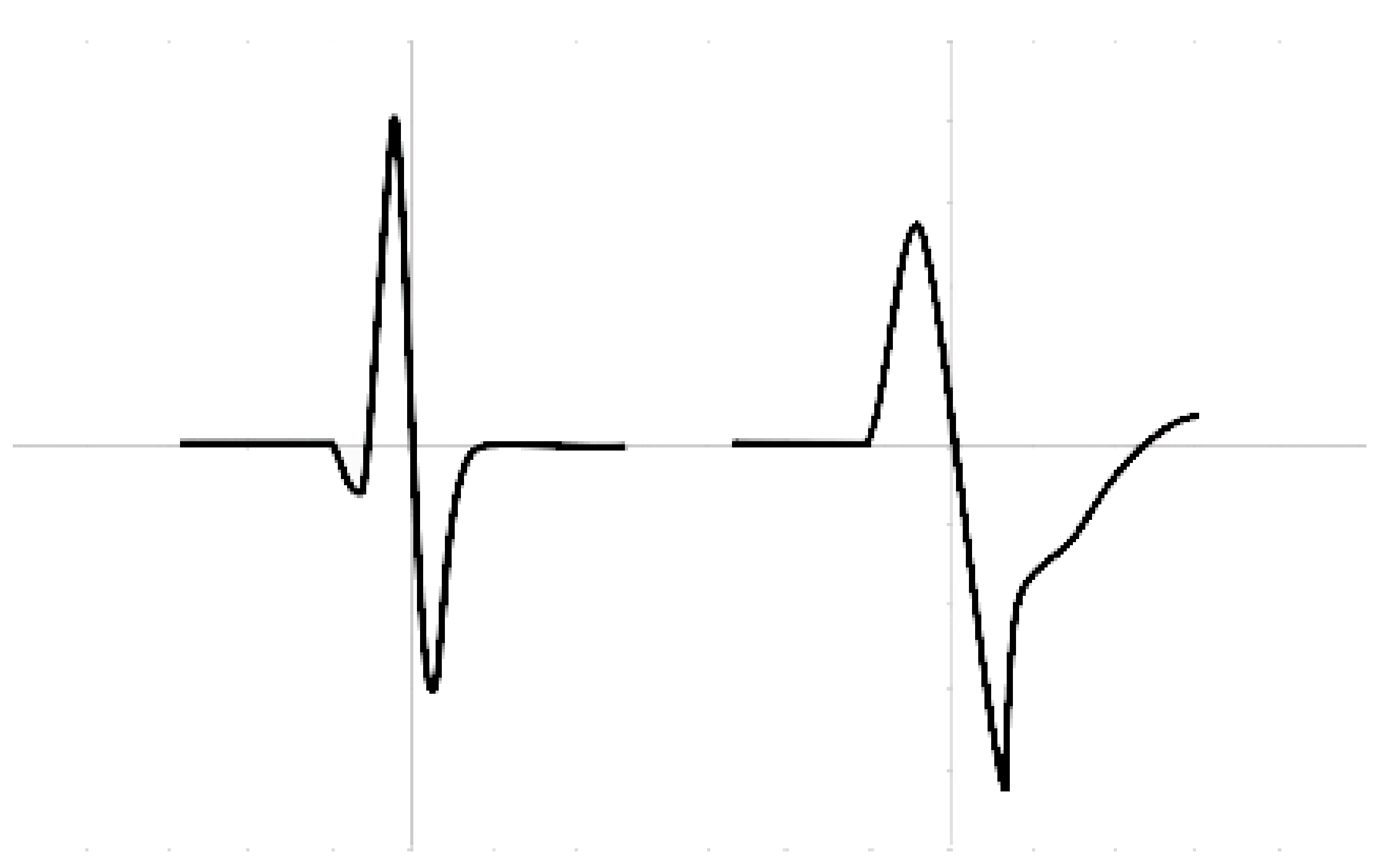
On an ECG, rhythm refers to the part of the heart that is controlling the initiation of electrical activity. Under normal circumstances, the sinoatrial node (SAN) initiates electrical activity because it undergoes spontaneous depolarization first at a rate of 60–100 bpm. When a rhythm originates from above the ventricles in the atria, it is termed a supraventricular (SVB) rhythm (narrow QRS or <120 ms), and when a rhythm originates from within the ventricles, it is termed a ventricular (VB) rhythm (broad QRS or >120 ms); these characteristics are represented in Figure 1.

The Association for the Advancement of Medical Instrumentation (AAMI) provides guidelines to classify heartbeats in an ECG signal into normal beats (N), supraventricular beats (SVB), ventricular beats (VB), fusion beats (FB), and unclassified beats (QB) [16,17]. However, because of their rarity in patients, the last two types of heartbeats are not usually included, and both QB and FB are relabeled simply as VB, leaving the task to classify only between NB, SVB, and VB.

An issue is the way research approaches the use of data sets. There are two accepted approaches to the problem, namely, inter- and intra-patient methodologies [18].

Works related to the inter-patient paradigm have lower performance against intra-patient works because of the use of different patients’ heartbeats in training, validation, and testing sets. However such works reflect the reality accurately since the inevitable variabilities among patients are incorporated in their results.

In this research, we present a review of previous work wherein it is shown that until nowm it has not been possible to overcome the variabilities among patients and train a generalized model from the databases available. The guidance of a physician is still needed to develop a patient adaptive model. This means that in the future, physicians would need to label new data because the signal for every individual patient changes in shape and heart rate, and the old parameters of the algorithm may need to be updated.

In this article, a novel unsupervised method is introduced that classifies between beats of supraventricular origin (SVBo), formed by the NB and SVB classes, and beats of ventricular origin (VBo), formed by the VB and FB. This approach does not require the assistance of a physician since it tries to capture the inherent patterns in the signal, and it uses heartbeat features from previous works across patients. Based on our experiments, it was concluded that this methodology works best when they are at least 40 VBo. The present approach may be used as a first step to distinguish between the remaining NB and SVB in future experiments.

The silhouette coefficient was implemented in MATLAB and used at the beginning to evaluate the quality of the clustering based on some parameters. For the experiments, an algorithm for clustering was implemented in MATLAB, and since this is an adaptive model for self-organizing maps, meaning that we could not use the silhouette score in general, and we would have to use it for every particular case or patient, which would yield just a distribution with no information worth for our purposes, as explained in Section 3.7, we chose between some parameters from the outcome that we derived from the comparison against the labels. In a future study with a modified algorithm, we aim to use the silhouette coefficient for the fine-tuning of the algorithm and better parameters.

2. Previous Research

Chazal et al. [19] extracted features in the time domain including heart rate and waveform descriptors of the ECG signal on both leads available in the MITBIH Arrhythmia Database. They used a linear discriminant classifier that outperforms their past work at that time. Llamedo et al. [20] presented a global classifier using the same training set as in Chazal et al. [19] but included two more databases to further test their method. He used the heart rate and features extracted from discrete wavelet transforms. He tested various sets of features and two different Bayesian linear classifiers ending with the linear discriminant classifier. Llamedo et al. [21] modified their past work to include more than two leads, using the same features and classifier. He used the INCART database in which every record has 12 leads. Using all the leads available, he outperformed their past work using this database. This is the only database available with 12 leads. Ye et al. [22] classified all types of heartbeats in the MITBIH database using the AAMI classification scheme. The morphological features used are coefficients of DWT and the result of applying independent components analysis, reducing the dimensionality with principal components analysis. The heart rate was also used as a feature. The classifier used is a support vector machine that combines the two leads of the MITBIH database. Once the features are extracted, the patients’ heartbeats are used for training and testing resulting in overoptimistic results of nearly 100%. However, the same model trained and tested as Chazal et al. [19] and Llamedo et al. [20,21] produced lower performance because of the variabilities among patients. Their results are comparable to Chazal et al. [19] and Llamedo et al. [20,21]. Mar et al. [23] principally worked on feature selection to classify ECG signals. They used a number of features in the temporal domain, morphological waveform features, statistical features, and features from the temporal–frequency domain using the DWT. The sequential forward floating search algorithm was used to determine relevant features, along with a linear discriminant classifier.

Once the optimal features are extracted, they are used to classify through a multilayer perceptron. The results are comparable to Chazal et al. [19], Llamedo et al. [20,21], and Ye et al. [22].

It is mentioned in [24] that general classification models are highly unreliable with ECG signals and are not widely used in practice. In order to overcome this problem faced by the intra-patient methodology, an adaptive patient model may be more effective because the patterns within a single patient are much easier to capture than in the inter-patient methodology. Such work involves the use of a certain number of beats previously labeled by a physician to train a learning algorithm. Works presented in [24,25] obtain results above 95% in almost all the cases, and some very close to 100%, in both precision and recall for the AAMI types of heartbeats.

Only Llamedo et al. [26] and Al Rahhal et al. [27] showed results without initial expert labeling. Wiens et al. [24] tested their algorithm developed using active learning with the same patients’ beats against the software from HAMILTON and with the advantage that it does not require data from the patient, but it only recognizes premature ventricular beats. Wiens et al. [24] outperformed HAMILTON. Llamedo et al. [26] modified their previous work in [21], which uses a general classifier by including a clustering algorithm, the K-means method. This modification slightly improves the performance, compared to their previous work, and also allows an expert to contribute to the output of the algorithm. The final results are around 95% with the help of the expert for each patient record. Al Rahhal et al. [27] used active classification through the deep learning approach. They suppressed the low frequency parts of the heartbeat and processed those employing an autoencoder algorithm to represent the signal in a lower dimension. A final softmax function is recorded similar to that in Chazal et al. [19], Llamedo et al. [20,21,27], Ye et al. [22], and Mar et al. [23]. Their results with beats labeled by an expert is close to 100% for every database they tested, while the automatic results when they used only the trained algorithm are much lower, representing the variability among patients. The only drawback is that a physician is needed to locate these labels on the ECG signal and as the heart’s beats rhythm and signals may change over time, future relabeling may be required to tune the trained model. Other interesting and related approaches are proposed in [15,28,29,30]; these deal with abnormalities in ECG segments based on supervised learning.

3. Materials and Methods

3.1. ECG Databases

All experiments were performed using selected records from public databases available in Physionet [31]. Each database has different files that correspond to the digitized signals, the information about the patients’ annotations, and the labels for heartbeats in the records. The following databases were used:

(a)

MIT-BIH Arrhythmia database (MITBIH), consisting of 48 half-hour signals recorded with two channels each one sampling at 360 samples per second with 11-bit resolution over 10 mV. The annotations for each heartbeat were made by cardiologists.

(b)

MIT-BIH Supraventricular Arrhythmia database (SUPRA), made up of 78 records, each 30 min long. Each record has two-lead signals, sampled at 120 Hz, with annotation files produced automatically first and then corrected by a medical student.

(c)

St. Petersburg Institute of Cardiological Technics (INCART) 12-lead Arrhythmia database, built up of 75 annotated records, each consisting of 12-lead signals sampled at 257 Hz for 30 min.

Following the labels suggested by the AAMI and the subsequent classification proposed in Llamedo and other works [20,21,26], the heartbeats were relabeled to NB, SB, and VB. For the purpose of this first unsupervised work, the later labels were changed to their anatomic origin in the heart as SVBo and VBo.

3.2. Summary Approach

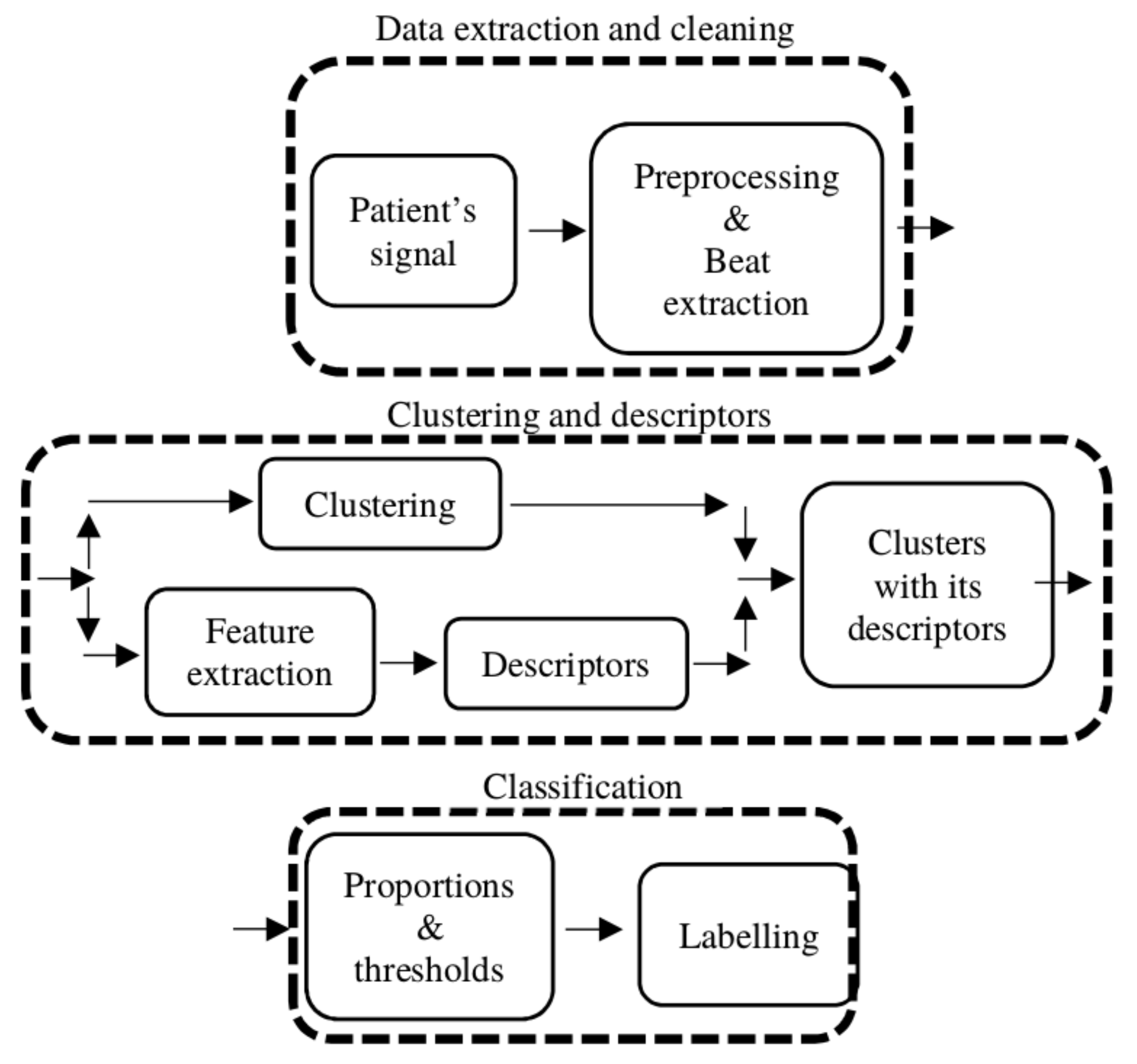
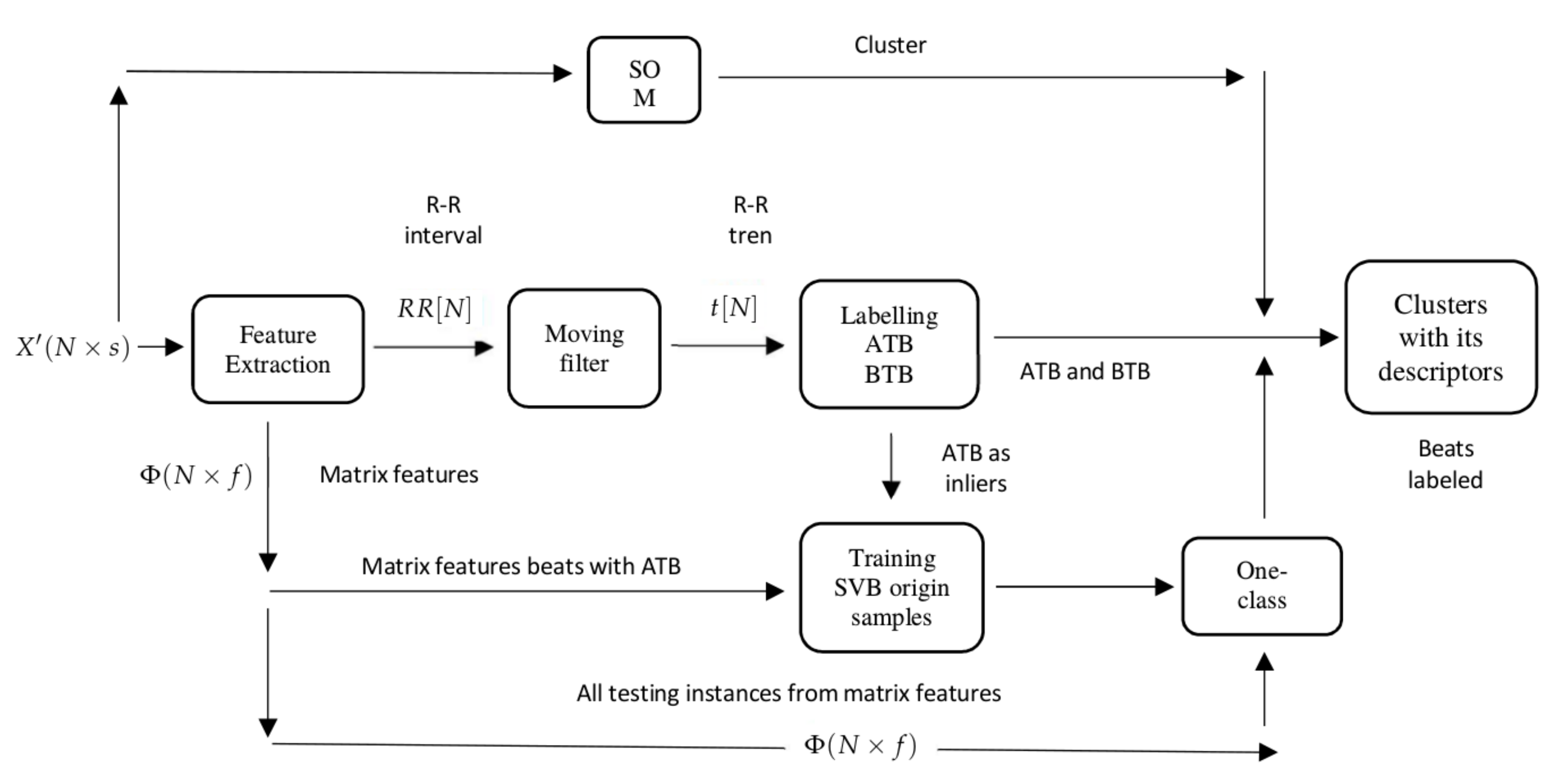
The algorithm requires a series of preprocessing and processing steps in order to cluster and distinguish the beats of supraventricular and ventricular origin. Figure 2 provides a high-level illustration of the processing pipeline divided into stages. In the first stage, Data extraction and cleaning, the patient signal is preprocessed and every beat of each record is sliced to form a matrix to work on. In stage 2, Clustering and descriptors, the clustering is performed and a set of different descriptors are computed to characterize each cluster (the expanded version of this stage is shown in Figure 3). The labeling processing is in stage 3, Classification, where the descriptors are used to compute a series of proportions for each cluster, and if these proportions reach a certain threshold, the cluster is classified as SVBo; otherwise, it is classified as VBo.

Three important assumptions for the algorithm are as follows:

(a)

With a significant number of VBo, the clustering algorithm is able to separate the signals;

(b)

If a trend is computed on the R–R interval signal, almost all the beats above this trend are going to be SVBo and most of the VBo occur below the trend, along with the rest of SVBo;

(c)

In the feature space, the SVBo signals are grouped together because they share similar waveform shapes, and the VBo signals are spread all over the feature space.

These assumptions were used to compute the descriptors and subsequently the proportions for the labeling of the clusters.

3.3. Data Extraction and Cleaning

The preprocessing of the signals is an important task to allow the extraction of useful information from them and for further analysis. The following four preprocessing procedures were performed:

(a)

Baseline wander removal;

(b)

Beat extraction;

(c)

Normalization;

(d)

Resample of signals.

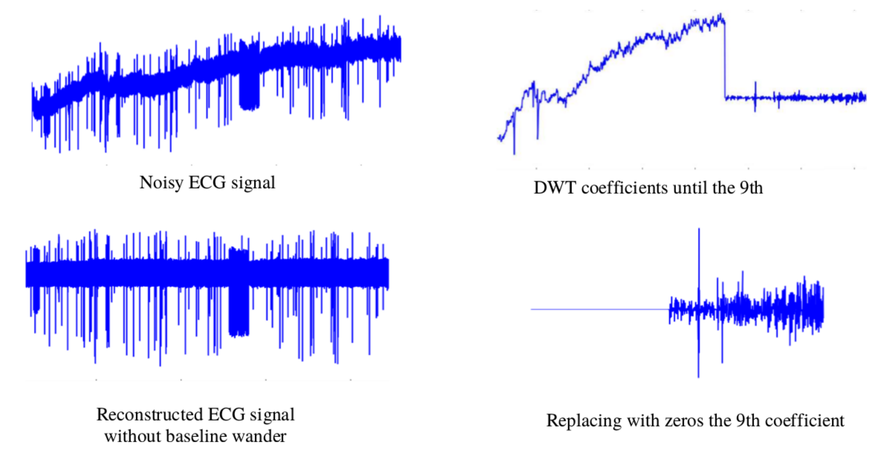
The baseline wander is generated by a low-frequency signal. Removing this noise benefits the extraction of time-domain features. For this task, the Discrete wavelet transform (DWT) is employed. Via the DWT coefficients, the ECG signal can be described in both time and frequency. The values of the coefficients are the results of passing the ECG signal through a series of high pass filters (HPFs) and low pass filters (LPFs). Depending on the wavelet applied, the LPF has specific coefficient values. The HPF is derived from the LPF as follows:

$$HPF[L-1-k]={[-1]}^{k}LPF\left[k\right]$$

(1)

where L is the length of the filter in the number of samples, and k are the coefficients of the filter. Each pair of filters can be represented as follows:

$$A\left[n\right]=\sum _{k=0}^{K}LPF\left[k\right]x[n-k]$$

(2)

$$D\left[n\right]=\sum _{k=0}^{K}HPF\left[k\right]x[n-k]$$

(3)

The filter has a half downsample after it to make the DWT efficient, represented as follows:

$$A_o\left[n\right]=A\left[2n\right]$$

(4)

$$D_o\left[n\right]=D\left[2n\right]$$

(5)

where n is the length of the signal produced. The DWT sends the signal through a cascade of HPF and LPF, resulting in an average signal detailed and differentiated for classification.

Following the recommendations in [32], the signal was decomposed into the ninth level using Daubechies wavelet family and the wavelet Daubechies 6 (db6), where the frequency in this level was about 0–0.351 Hz [32] levels of resolution. The signal proceeds through all the necessary levels to isolate the energy of the noise. To eliminate the baseline wander from the ECG, the signal was constructed from the eighth coefficient to the first, replacing the coefficients of the ninth with zeros. Figure 4 shows the denoising process of the ECG signal.

The heartbeats were extracted from the denoised signal. Every record had a file indicating the heartbeat location in the sample and its type. After analyzing the research and results of Martis et al. [32], which uses a window of approximately 552 ms and the research and results of Marinucci et al. [33] that uses a window of 700 ms, in our case, we considered a slightly wider window, i.e., 730 ms–330 ms before the R peak and 400 ms after it—which were enough to cover the heartbeats of our test signals, making sure the whole beat and its characteristic waveform are totally covered. Every beat has a length of 0.73 s but because the sampling frequency varies among the databases, the length in samples varies depending on the database employed:

(a)

MITBIH ECG signals consisted of 263 samples;

(b)

INCART consisted of 188 samples;

(c)

SUPRA had 93 samples.

Finally, the signal values were normalized between 0 and 1 and resampled at 360 Hz, the sampling frequency of the MITBIH database signals. This was carried out following the recommendations of Llamedo et al. [26].

3.4. Clustering and Descriptors

In the clustering and descriptors step, three major procedures were performed according to the assumptions previously stated.

Firstly, the signals were clustered in groups. This work proposes that the clustering algorithm, self-organizing maps (SOM), is able to distinguish between SVBo and VBo, then the problem is reduced to classifying the clusters in SVBo or VBo using a set of descriptors. The SOM is an arrangement of neurons connected in a single-layer network, with most of the cases presented in a two-dimensional network. It is characterized by soft competition between neurons in the output layer, where a winner neuron and its neighbors are updated at every iteration in the training. The SOM learns the distribution and topology of the input vectors, generally mapping data $R^n$ onto a regular bidimensional grid. A parametric reference vector $m_i\in R^n$ is associated with every node i in the map. Every input x is compared with every node, and the closest match is selected, and then the input is mapped onto that location $c=argmi{n}_i\parallel x-m_i\parallel$. Nodes topographically close to others in the array will learn from the same input with the following formula:

$$m_i(t+1)=m_i\left(t\right)+\infty *h_{c,i}\left(t\right)[x\left(t\right)-m_i\left(t\right)]$$

(6)

The heartbeats extracted are sliced from the 60th to 170th sample and clustered, using the self-organizing map (SOM) algorithm. The time frame extracted from the heartbeats ensures that the hearbeat QRS complex is used for clustering, which is an important differentiator between the SVBo and VBo.

Secondly, this work stated that if we computed the trend of the heart rate in a window time, most of the heartbeats above the trend are SVBo, and most of the VBo will be located below the trend. The heart rate is computed taking the distance in samples from the heartbeats that the R peak selected and the previous one. All databases identify a heartbeat with its R peak location; thus, every R peak is already identified in the data. The trend $t\left[N\right]$ is computed using a moving average filter as follows:

$$y\left[n\right]=\sum _{k=0}^{K}w\left[k\right]x[n-k]$$

(7)

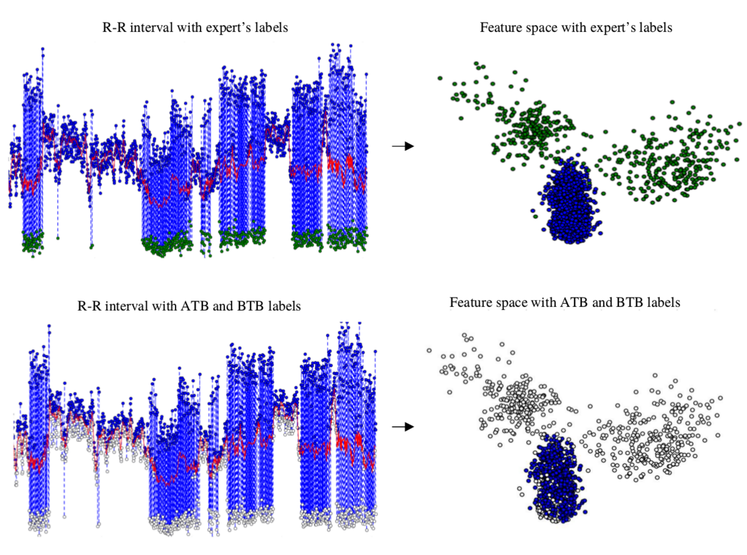
where k represents the index terms of the signal, $w\left[k\right]$ represents the window signal, $x[n-k]$ is the signal value that is being filtered shifting k terms, and $y\left[n\right]$ is the filtered output signal. RR features such as mean, kurtosis, and SD were not part of the inputs for final clustering. RR intervals as features were used as an initial reference to preclassify the clusters as “normal” if they were above the red trend line, as can be seen in Figure 5 and explained in Section 3.4.

The beats above the trend level are labeled as above-the-trend beats (ATBs), and they are used in the third step as SVBo, and all those below are labeled as below-the-trend beats (BTBs). These labels become descriptors for each cluster. In Figure 5, a patient’s R–R interval, its trend, and the labeling of ATB and BTB in the heart rate are shown.

The third assumption is that, in the feature space, most of SVBo are grouped and VBo are scattered. With the help of the second assumption, most heartbeats identified above the trend are labeled as SVBo and with this one class, the one-class SVM (OC-SVM) classifier algorithm is trained to create a nonlinear discriminant function to include more SVBo, and the rest of the heartbeats are classified as VBo. The OC-SVM separates the data using a subset of the class identified as reference for outliers by some prior value specified $v\in (0,1)$. The solution is to estimate a function f, which is a discriminant between the points marked as outliers and the insiders. The function f can be seen as

$$f\left(x\right)=\left\{\begin{array}{cc}{SVM}_o\hfill & \mathrm{if}x\in S\hfill \\ {VB}_o\hfill & \mathrm{if}x\in \overline{S}\hfill \end{array}\right.$$

(8)

where the ${SVM}_o$ are identified as the subset inside the function and VBo outside. For this, it is necessary to resolve the quadratic programming function

$$min\left(\frac{1}{2}{\parallel w\parallel }^2+\frac{1}{vN}\sum _{i=1}^N{\xi }_i-\rho \right)$$

(9)

subject to

$$\begin{array}{c}\hfill w·\varphi \left(x_i\right)⩾\rho -{\xi }_i\\ \hfill i=1,2,\dots ,N\\ \hfill x_i⩾0\end{array}$$

where $\varphi :X\to H$ represents a kernel map, which transforms the training examples to another space, N is the maximum number of training samples, w and $\rho$ are the weight and offset parameterizing the hyperplane in the feature space, and ${\xi }_i$ is the classic slack variable from the standard support vector machines to prevent over-fitting.

Resolving the quadratic problem, the decision boundary is as follows:

$$f\left(x\right)=sign(w·\varphi \left(x_i\right)-\rho )$$

(10)

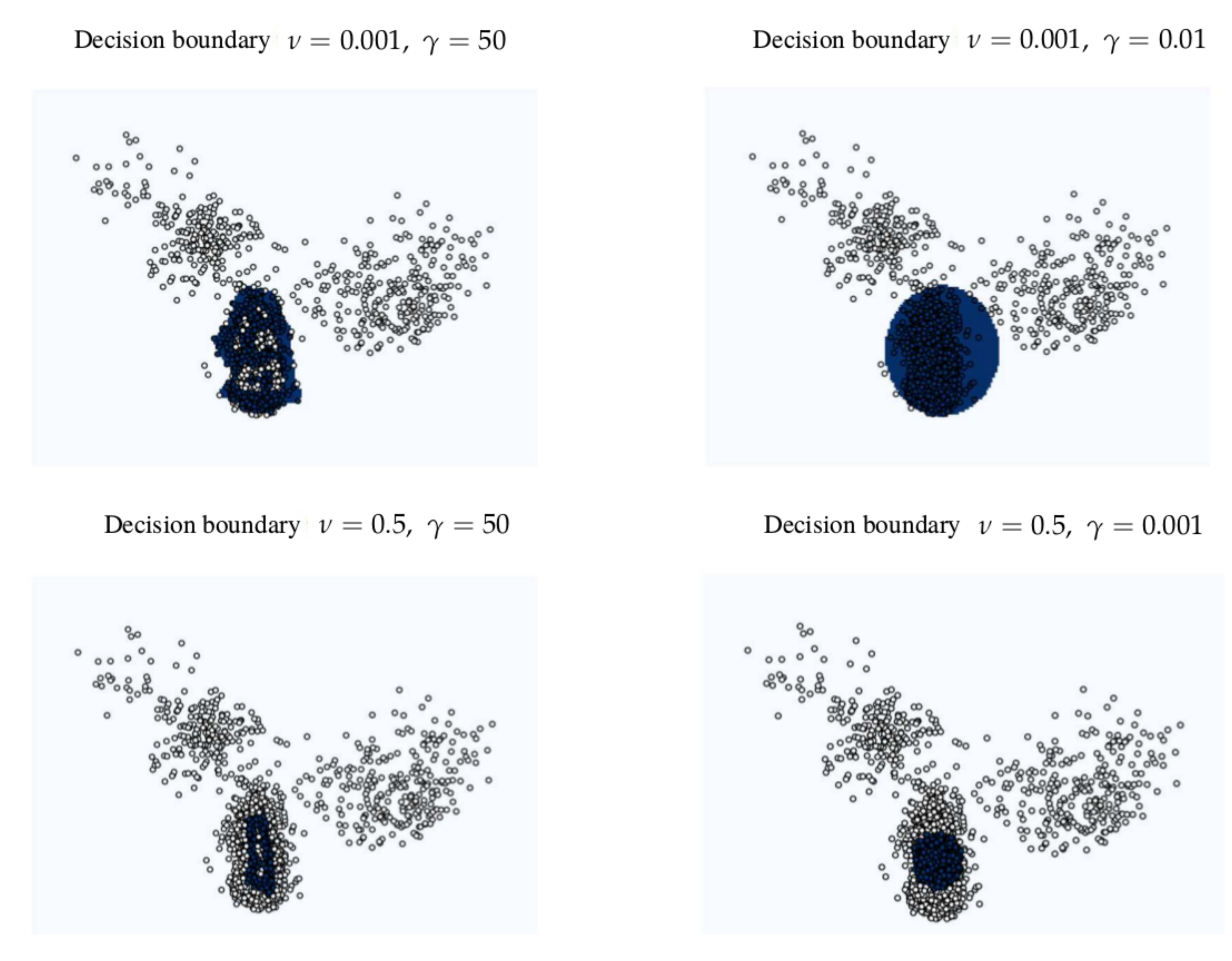
The matrix $X^{\prime }\left(s\right)\in R^{N\times S}$ containing the heartbeats is converted into feature space $\mathsf{\Phi }(N\times f)$, where f is the feature dimension used. In this work, different sets of features were used in experimentation and will be explained in the next sections. In order to help to distinguish which clusters are SVBo or VBo, a partial number of SVBo are identified utilizing One-Class SVM. The ATBs are used as SVBo class, the only class in this step, and the OC-SVM creates a discriminant function to englobe similar heartbeats. Furthermore, Figure 5 shows the beats above the trend located in a feature space. Figure 6 shows different decision boundaries in a feature space created with different hyperparameters in the OC-SVM. The beats identified as SVBo from the one-class SVM serve as well as descriptors to characterize each cluster.

In

Table 1. Example of ECG signal separated in clusters and its descriptors.

Cluster (clj)	# Beats in Cluster (clj)	# ATB in Cluster (clj)	# BTB in Cluster (clj)	# SVBo Identified
1	227	0	227	0
2	292	195	97	273
3	346	216	130	221
4	478	316	162	385
5	451	299	152	394
6	229	0	229	0

, an example of data separated in clusters with its descriptors is displayed; this is from the same signal used for Figure 5 and Figure 6.

3.5. Classification

To determine if a cluster ${cl}^j$ is SVBo or VBo, three proportions $P_i^{{cl}^j}$, where $i=1,2,3$ and ${cl}^j$ is a cluster, are computed using the descriptors previously defined. Each proportion $P_i^{{cl}^j}$ is compared with its corresponding $d_i$ threshold and the results from the comparisons are used to label that ${cl}^j$ as SVBo or VBo. The first proportion, $P_1^{{cl}^j}$ is computed as follows in Equation (11):

$$P_1^{{cl}^j}=\frac{\#\mathrm{SVBo}}{\#\mathrm{beats}\mathrm{in}{cl}^j}$$

(11)

This proportion is the percentage of SVBo identified in the cluster by the one-class SVM algorithm. If the proportion surpasses the threshold $d_1$, then the $c{l}^j$ is labeled as being SVBo.

The second proportion, $P_2^{{cl}^j}$ is shown in the next Equation (12).

$$P_2^{{cl}^j}=\frac{\#\mathrm{SVBo}}{\#\mathrm{beats}\mathrm{in}{cl}^j}$$

(12)

This proportion represents the error of the one-class SVM in labeling the SVBo or the error of SOM clustering SVBo with VBo. It is expected that clusters that are VBo only have mostly BTB and much less ATB. However, some of SVBo may be mixed in a cluster of VBo, and the one-class SVM may identify them as VBos. In such cases, comparing the rate between the number of SVBo in this cluster and the total number of BTB with its threshold $d_2$ tells us what type of cluster it is. A majority of BTB will not let the proportion reach the threshold. If the cluster does not contain any BTB, this proportion is not computed. $P_3^{{cl}^j}$ is shown in (13).

$$P_3^{{cl}^j}=\frac{\#\mathrm{ATB}}{\#\mathrm{beats}\mathrm{in}{cl}^j}$$

(13)

Lastly, as mentioned before, because it is hypothesized that most of the ATBs are SVBo because a great number of beats are NB in many signals, this rate represents the relation between the ATB and the number of beats in this cluster. The values of the thresholds are determined experimentally, as will be explained. If any of these thresholds are reached, the cluster is labeled as SVBo; otherwise, it is represented as VB.

3.6. Hyperparameters and Features

The approach has a great number of hyperparameters, changing their values may change the output of the approach. The SOMs parameters include the following:

• Type of grid for cluster nodes;
• Number of neurons;
• Number of neighbors;
• Number of iterations;
• Learning rate.

As the SOM is a clustering algorithm, in this case, a reproducibility experiment was performed to ensure that the results can be reproduced multiple times to guarantee its use outside this study.

The one-class SVM has the hyperparameter $\nu$, which determines the proportion of beats outside of the decision function. The kernel employs the radial basis function (RBF) that uses the $\gamma$ hyperparameter, which plays an important role in determining the decision boundary.

Additionally, the threshold $d_i$ to determine if a cluster is SVBo or VBo needs to be specified as well.

The default hyperparameters used for SOM training have a neighbor size of 3 and a hexagonal grid topology with 200 iterations.

Furthermore, the hyperparameters whose values are determined experimentally are as follows:

• The dimension of the grid of SOM;
• The $\nu$ in the One-Class SVM algorithm;
• $\gamma$ for the RBF kernel;
• The thresholds $d_i$.

Different subsets of features were extracted and merged together to form the final features set to be experimented with to reach the highest classification performance. The first feature subset is the DWT db3 coefficients of the QRS complex; the second feature subset is DWT db6 coefficients of the whole beat; the third feature subset feature is statistical computations of the sections before, after, and within the QRS complex; the fourth feature subset is the statistical computations of the QRS complex. The statistical computations are the mean, the standard deviation, the maximum, the minimum, the skewness, and the kurtosis. The final feature sets to experiment with were as follows: feature set 1 is the PCA transformation of the first features subset; feature set 2 is the PCA transformation of the second feature subset; feature set 3 is the merged of the first and fourth feature subsets; feature set 4 is the fourth feature subset; feature set 5 is the PCA transformation of the third feature subset; feature set 6 is the merged of the first and third feature subsets; features set 7 is the merge of the second and fourth feature subsets.

Table 2. Subset and Set of Features Formed.

Features	Description
subset feature 1	QRS complex + DWT db3
subset feature 2	Whole beat + DWT db6
subset feature 3	Sections + SO + HOS
subset feature 4	QRS complex + SO + HOS
feature set 1	feature 1 + PCA
feature set 2	feature 2 + PCA
feature set 3	feature 1 + feature 4
feature set 4	feature 4
feature set 5	feature 3 + PCA
feature set 6	feature 1 + feature 3
feature set 7	feature 2 + feature 4

summarizes the basic features and the set of features created with all these.

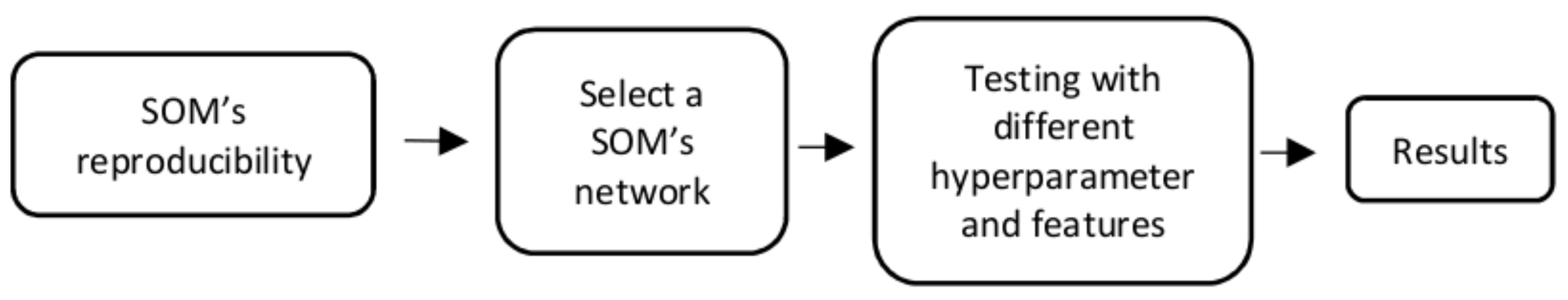
3.7. Experimentation Setup

Figure 7 shows the experimental setup. First, five types of topologies were used in SOM to determine which one is more appropriate for the given data: $2\times 2$, $3\times 2$, $3\times 3$, $4\times 3$, and $4\times 4$. Each type of SOM was run five times using the set of the default hyperparameters ($\nu =0.1$, $\gamma =1.5$, $d_1=0.5$, $d_2=0.7$, and $d_3=0.3$) and with the default set of features (DWT + PCA of the QRS complex of the signals) to determine the reproducibility of the results. These parameter values and features were selected because they produce good results in the first trials. Experimenting with these variables as defaults gave us an insight into the proper topology to use for this task.

Once a topology was selected, the set of features and parameters were determined first using three different values for each hyperparameter for each set of features for each database, and the best three sets of features were selected. Then, we experimented with five different values of hyperparameters and the best one was selected to obtain the final results to compare it with prior works.

3.8. Evaluation

Because of the high imbalance among the classes, the results are in terms of sensitivity (S) also known as recall and positive predictive value ($P^{+}$) also known precision, as presented in [26]. In addition, the F-score is presented here, which is the harmonic mean of these two parameters. F-score is computed as given in Equation (14).

$$F=2*\frac{S\times P^{+}}{S+P^{+}}$$

(14)

The F-score (F) can be seen as a measure of combined performance involving both S and $P^{+}$. With values between 0 and 1, highest performance with 1, each S and $P^{+}$ needs to be high to have a high F-score. In other words, it involves a balance between these two performance measures.

The searches for the best SOM topology and the best set of features and parameters values possible result in a great number of results in terms of S, $P^{+}$, and F. As for specific values of parameters and specific selection of features, the performance varies for each database, and changing these can cause increased or decreased performances.

The purpose of these experiments is to set the hyperparameters’ values that can maintain the best balance possible among the performance for the three databases. To achieve this, a modification of the F-score formula is made to compare the performance of each F-score for each database. We call it F-general ($Fg$), and the equation is shown in (15).

$$Fg=3*\frac{F_{SUPRA}\times F_{MITBIH}\times F_{INCART}}{F_{SUPRA}+F_{MITBIH}+F_{INCART}}$$

(15)

This equation is motivated by the way F-score is computed, from a precision value and recall. It is also a harmonic mean of the three F-scores for the three databases. The reason we used this equation is that we looked for hyperparameters and features not biased towards any of the databases. The purpose is to have a generalized set of hyperparameters and features that could balance the performance among the databases. This equation was applied to select the SOM network, the hyperparameters, and set of features.

4. Results

Table 3. SOM Reproducibility Experiments Results.

	SOM Topology	VBo	SVBo	VBo
		S	P+	S	P+	F Score
SUPRA	2 × 2	0.85905	0.78189	0.98632	0.99191	0.81866
		0.0002	0.00052	0.00004	0.00001	0.0003
	3 × 2	0.89814	0.79383	0.98654	0.99115	0.84277
		0.00216	0.00071	0.00019	0.00407	0.00109
	3 × 3	0.89386	0.77637	0.9853	0.99389	0.83095
		0.0046	0.00717	0.00067	0.00026	0.00299
	4 × 3	0.87991	0.79268	0.98368	0.99083	0.7909
		0.03701	0.09298	0.00667	0.00414	0.00551
	4 × 4	0.90934	0.68555	0.97617	0.99473	0.78168
		0.00798	0.014	0.00152	0.00046	0.01005
MITBIH	2 × 2	0.8075	0.94047	0.99576	0.98423	0.86893
		0.00027	0.00013	0.00001	0.00002	0.00021
	3 × 2	0.83549	0.91752	0.99377	0.986	0.87458
		0.00108	0.0031	0.00026	0.001	0.00116
	3 × 3	0.84905	0.88435	0.99078	0.98753	0.86631
		0.00207	0.00994	0.00092	0.00016	0.00378
	4 × 3	0.8544	0.84955	0.98738	0.98792	0.85177
		0.00229	0.02786	0.00273	0.00018	0.01351
	4 × 4	0.86079	0.85686	0.98807	0.98845	0.85879
		0.0023	0.01002	0.001	0.00018	0.00436
INCART	2 × 2	0.89461	0.94787	0.9936	0.9864	0.92047
		0.00119	0.0005	0.00006	0.00015	0.00071
	3 × 2	0.92128	0.91843	0.98936	0.98976	0.91985
		0.00178	0.00336	0.00048	0.00023	0.00188
	3 × 3	0.92325	0.88574	0.98452	0.98997	0.9041
		0.00231	0.00296	0.00043	0.0003	0.00231
	4 × 3	0.92732	0.86486	0.98116	0.99046	0.89498
		0.00226	0.00752	0.00122	0.00029	0.00381
	4 × 4	0.92359	0.87453	0.98277	0.99	0.89839
		0.00042	0.00249	0.00039	0.00005	0.00129

shows the results of inserting every patients’ signal through the algorithm for each network topology proposed with the default hyperparameters and set of features.

In order to ensure the reproducibility of the results, in terms of S and $P^{+}$, the mean and the standard deviation were taken from the five runs of every database for every network topology.

It can be seen that the standard deviation from the runs of every topology of every database has a value near zero, which means minimum or insignificant changes between the results within the topology but not between topologies.

In order to select one,

Table 4. Selecting the Best of SOM Topology.

	SUPRA	MITBIH	INCART	F-General
2 × 2	0.81866	0.86893	0.92047	0.75318503
3 × 2	0.84277	0.87458	0.91985	0.77126533
3 × 3	0.83095	0.86631	0.9041	0.75056012
4 × 3	0.7909	0.85177	0.89498	0.71276568
4 × 4	0.78168	0.85879	0.89839	0.71262883

presents the F of the VB origin because the results in the SVB origin are nearly 1 in every database. For the SUPRA database, the two F highest values are obtained with the topologies $3\times 2$, and $3\times 3$ with 0.8427 and 0.8309, respectively. With the MITBIH database, the highest valued topologies are $2\times 2$, $3\times 2$ and $3\times 3$, with F-scores of 0.8689, 0.8745, and 0.8663, respectively. The INCART database produces the highest values with the $2\times 2$ and $3\times 2$ topologies, with 0.9204 and 0.9198 F-scores values, respectively. The $3\times 2$ topology has the highest performances for SUPRA and MITBIH databases compared to other topologies, while for INCART, the $2\times 2$ topology is just slightly above $3\times 2$. However, the $Fg$ of each database shows that the $3\times 2$ topology has the highest performance for the three databases, and because of that, this SOM network was used to run the next experiments involving the selection of the parameters and set of features.

As the default parameters gave good results in the first tests, other similar and close values were tested as upper and lower bound values, with sets of features as presented before, in order to find better combination of hyperparameters and features to improve our results. The test values for each parameter are as follows: $\nu =0.001$, 0.1, 0.5; $\gamma =0.001$, 1.5, 3; $d_1=0.4$, 0.5, 0.6; $d_2=0.5$, 0.6, 0.7; $d_3=0.2$, 0.3, 0.4. Each parameter has three different values, giving rise to 243 experiments for each set of features for each record in every database. In each experiment, the S, $P^{+}$, and F for each set of features (for each database) were computed, and only the highest performance in terms of F are shown in

Table 5. Selecting the Best Three Features.

	SUPRA	MITBIH	INCART	F-General
feature	0.8892	0.8755	0.9214	0.801129807
set 1
feature	0.8602	0.8755	0.928	0.787117392
set 2
feature	0.8892	0.8755	0.9214	0.801129807
set 3
feature	0.8957	0.8723	0.9468	0.817466775
set 4
feature	0.8946	0.8721	0.8687	0.771506723
set 5
feature	0.8184	0.7725	0.9029	0.686694226
set 6
feature	0.8608	0.8721	0.8919	0.765261291
set 7

.

Results with the highest values are in Table 5, and these are presented for each set of features. For example, parameters for feature set $1=\nu =0.1$, $\gamma =1.5$, $d_1=0.4$, $d_2=0.5$, $d_3=0.3$. The $Fg$ is computed from with each VBos F of every database for every set of features. The best three were set of features 1, 3, and 4. It is important to mention that these features involve only the QRS complex, which, in fact, is very accurate medically in distinguishing the heartbeat between SVBo and VBo.

As the hyperparameters values for the three different sets of features were nearly the same, just varying $d_2=0.6$ in feature set 4 and $d_2=0.5$ in feature set 1 and 3, the final hyperpameter values to experiment with were as follows: $\nu =0.05$, 0.1, 0.15, 0.25, 0.3; $\gamma =1$, 1.25, 1.5, 2, 2.5; $d_1=0.3$, 0.35, 0.4, 0.45, 0.5; $d_2=0.55$, 0.575, 0.6, 0.625, 0.65; $d_3=0.25$, 0.275, 0.3, 0.325, 0.35. In this case, 3125 experiments were performed for each set of features for each database.

In order to select the best set of features with parameters,

Table 6. Example of ECG signal separated in clusters and its descriptors.

	SUPRA	MITBIH	INCART	F-General
feature	0.9005	0.8655	0.9276	0.80519243
set 1
feature	0.8892	0.8862	0.9187	0.80614369
set 3
feature	0.89569357	0.8862	0.9394	0.8220299
set 4

presents the $Fg$ values computed with the highest F for each database for each set of features. The hyperparameters of each feature set presented the best F were as follows: feature set 1 = $\nu =0.05$, $\gamma =2.25$, $d_1=0.45$, $d_2=0.55$, $d_3=0.35$; feature set 3 = $\nu =0.1$, $\gamma =1.25$, $d_1=0.3$, $d_2=0.55$, $d_3=0.3$; feature set 4 = $\nu =0.15$, $\gamma =1$, $d_1=0.35$, $d_2=0.55$, $d_3=0.3$. It has to be noticed that even though these set of features were selected with almost the same parameters values, they ended up with completely different and $Fg$ values. The best set of features with its parameters was feature set 4, with 0.8220%. With this, the experimentation concludes with a SOM network of $3\times 2$ neurons, with feature set 4 and the parameters $\nu =0.15$, $\gamma =1$, $d_1=0.35$, $d_2=0.55$, $d_3=0.3$.

The results of all the databases are compared with similar works in

Table 7. Comparing results with similar works.

Type of Model	Data	Work	NB		SVB		SVBo (N B and SVB)		VBo (VB and FB)		F-Score for VBo
			S	P+	S	P+	S	P+	S	P+
Generalized Models	MITBIH-AR DS2	Mar [9]	0.90	0.99	0.83	0.34			0.87	0.61	0.7171
		Chazal [5]	87	99	0.759	0.385			0.777	0.819	0.7974
		Llamedo [7]			0.77	0.39			0.81	0.87	0.8389
		Ye [8]			0.608	0.523			0.815	0.631	0.7112
		This work					0.9996	0.9848	0.8039	0.9945	0.8891
Patient adaptive (no training data from the same patient)	MITBIH-AR DS2	Llamedo [11]	0.93 ± 0	0.99 ± 0	0.77 ± 0	0.39 ± 0			0.82 ± 0	0.70 ± 0	0.7552
		This work					0.9996	0.9848	0.8039	0.9945	0.8891
	MITBIH-AR common tests records	Al Rahhal [12]			0.115	0.132			0.847	0.871	0.8588
		This work					0.9928	0.9797	0.8309	0.9335	0.8792
	MITBIH	Llamedo [11]	0.96 ± 0	0.98 ± 0	0.76 ± 2	0.43 ± 2			0.80 ± 2	0.82 ± 3	0.8098
		Al Rahhal [12]			0.41	0.429			0.91	0.795	0.8486
		HAMILTON [10]							0.928	0.795	0.8563
		This work					0.9957	0.9865	0.8360	0.9428	0.8862
	SUPRA	Llamedo [11]	0.94 ± 0	0.97 ± 0	0.47 ± 3	0.50 ± 1			0.82 ± 0	0.54 ± 1	0.6511
		Al Rahhal [12]			0.880	0.1431			0.6519	0.931	0.1639
		This work					0.9938	0.9941	0.8981	0.8930	0.8956
	INCART	Llamedo [11]	0.89 ± 0	0.99 ± 0	0.74 ± 4	0.8 ± 0			0.88 ± 0	0.96 ± 1	0.9182
		Al Rahhal [12]			0.1558	0.0254			0.7511	0.3763	0.5013
		This work					0.9946	0.9899	0.9220	0.9575	0.9394

. The approach was tested also with two databases derived from the MITBIH database, as in [21,27]. Even though some other authors such as Kiranyaz et al. [34] claim that the average detection accuracies of both VB and SPV ectopic beats were over 97% using the MIT-BIH arrhythmia database, for both training and testing of the algorithm, this shows that the supervised algorithms so far continue being of higher precision or accuracy.

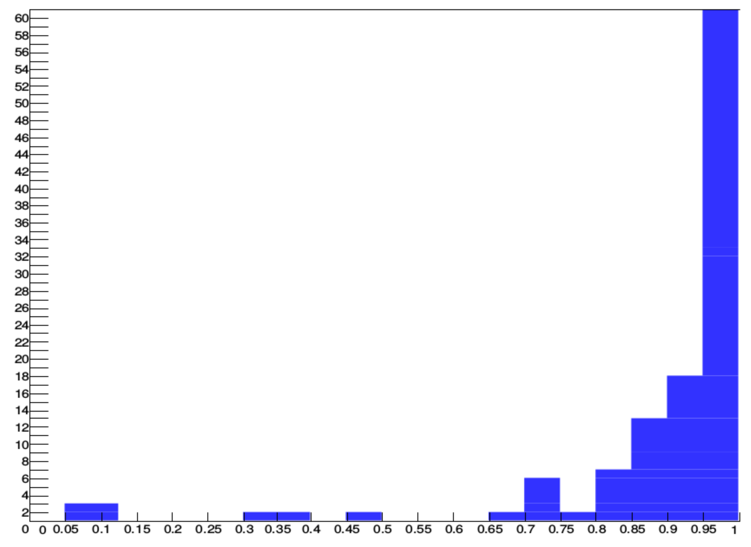
In Figure 8, the performance of the algorithm for 109 records that have at least 40 VBos is shown. The histogram shows that 89 out of 109 records have at least a 0.85 F-score, and 60 out of 109 are over 0.95 F-score. These records are 30 min long; in other words, there are approximately 1500 and up to 2500 heartbeats depending on the heart rate. These records represent most of the VBos in the three databases.

5. Discussion

One of the main differences among all works is the percentage of $P^{+}$ in VBo, where our approach produces percentages above 90%, with the exception of the SUPRA database with 0.8930%. This means that a great number of beats classified as VBo are indeed VBo.

The F-score of this work outperforms the general classifier models. Martis et al. [23] and Ye et al. [22] present the lowest F-score because of their $P^{+}$ around 0.60, plunging the F-score value, while Chazal et al. [19] and Llamedo et al. [20] maintain similar values for both S and $P^{+}$, with F-score of 0.79 and 0.83 respectively. The inevitable variability between patients lowers the performance of these general classifiers. The results for this work are higher, with 0.88, because it presents a $P^{+}$ near 100%.

An additional comparison is made with works where they present models that can be adapted to a patient. The results to be compared are the models before physician’s help is provided for the adaptive algorithms, otherwise, their results are nearly 95%. Only Llamedo et al. [26] and Al Rahhal et al. [27] presented this type of results, and Wiens et al. [24] presented the performance of the HAMILTON software on the MITBIH database for comparative results. As in the general models, the performance on the F-score for VBo in the algorithm proposed was superior over these methods. No patterns in their results exist showing misclassification measurements, which vary depending on the database. For example, Llamedo presents balanced results in the MIIBIH database, while a very low 0.54 in $P^{+}$ is presented in the SUPRA database, and in the INCART database, the $P^{+}$ is 0.96 against a 0.88 for S. Meanwhile, Al Ranhal et al. [27] have very similar results with the HAMILTON software, with a low performance of 0.79% for the MITBIH database in $P^{+}$, 0.93 for the SUPRA database for the same measurement, and very lower, 0.37, in the INCART database. Our approach has higher performance because it maintains an S always above 0.9 for $P^{+}$ in every database; in this way, the derived F-score presents a superior performance. Overall, our approach has produced better results in F-score for VBo, compared to these studies.

The physicians’ need for constant monitoring of the arrhythmias presented the opportunity for the creation of algorithms or methodologies that perform automatic measurements of arrythmia. Different approaches have been used by the scientific community, such as the intra- and inter-patient paradigms. Such approaches have historically employed manual data tagging by an expert. The works of Llamedo et al. [20] and Al Rahhal et al. [27] were the first to show results from prelabeled data.

Those studies showed progress, compared to previous studies, but they maintained the limitation of not being able to overcome the variations between patients or to train a general model that uses the available databases, as explained in Section 3.1. Our work introduces a new unsupervised method that classifies beats of SVBo origin, formed by classes NB and SVB, and beats of ventricular origin VBo, formed by VB and FB. This method does not require the assistance of an expert physician, as it captures the inherent patterns found in the captured signal and makes use of the heartbeat characteristics captured from previous patient studies.

Previous works need labels in order to create a heartbeat classifier. A general classifier, created by heartbeat samples from other patients, may not be the best solution as the inevitable variability lowers the performance of the classifier. Even though the adaptive patient classifiers are a promising solution in classifying arrhythmias, it needs a physician to identify a certain number of heartbeats to feed the algorithm for every patient.

In this work, a new unsupervised algorithm was proposed to classify between supraventricular and ventricular heartbeats in a single patient, in a window time, without previous labels provided by a physician.

Three assumptions were proposed to implement this algorithm. A never used one was that most of the heartbeats above a computed trend in the heart rate are of supraventricular nature. This can be used as a new feature in future works.

6. Conclusions

In this work, a new unsupervised algorithm was proposed to classify between supraventricular and ventricular heartbeats without the need for any labeling by a physician. A new feature is using as a reference the trend in the heart rate to classify the heartbeats above that trend as of “supraventricular” nature.

The results of this algorithm show better performance against other generalized models and/or adaptive patient models without the need for a physician’s assistance.

These results show a promising path for unsupervised models to classify these types of heartbeats, and it can be seen as a milestone to develop further stages for classification between supraventricular heartbeats and normal heartbeats.

This comes from the fact that this model adapts itself to the patient’s heartbeats waveform. Our algorithm works better without the need for a large number of VBo heartbeats. These results show a promising path for unsupervised models to be used as classifying indicators for SVBo and VBo types of heartbeats.

No other similar work has been developed thus far, though some improvements in the algorithm are needed to reach higher performance in precision and recall metrics. Although the purpose of this research is to develop an adaptive system granting better results, compared to those from other authors, we also concluded that the silhouette criterion can be applied in a new research study or proposal in the classification of ECG signals, which, to the best of our knowledge, nobody has performed thus far.