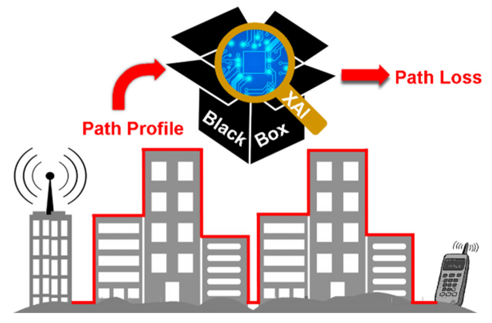
Explainable Deep-Learning-Based Path Loss Prediction from Path Profiles in Urban Environments

Abstract

This paper applies a deep learning approach to model the mechanism of path loss based on the path profile in urban propagation environments for 5G cellular communication systems. The proposed method combines the log-distance path loss model for line-of-sight propagation scenarios and a deep-learning-based model for non-line-of-sight cases. Simulation results show that the proposed path loss model outperforms the conventional models when operating in the 3.5 GHz frequency band. The standard deviation of prediction error was reduced by 34% when compared to the conventional models. To explain the internal behavior of the proposed deep-learning-based model, which is a black box in nature, eight relevant features were selected to model the path loss based on a linear regression approach. Simulation results show that the accuracy of the explanatory model reached 72% when it was used to explain the proposed deep learning model. Furthermore, the proposed deep learning model was also evaluated in a non-standalone 5G New Radio network in the urban environment of Taipei City. The real-world measurements show that the standard deviation of prediction error can be reduced by 30–43% when compared to the conventional models. In addition, the transparency of the proposed deep learning model reached 63% in the realistic 5G network.

1. Introduction

The emerging fifth-generation (5G) mobile communication systems are expected to bring a complete revolution in applications and experiences [1]. Mobile operators worldwide are racing to roll out 5G services. However, among the technical challenges, accurate channel models to predict path loss are vital for the design of 5G cellular communication systems.

Many path loss models for wireless communication networks have been studied by prior researchers. Popoola et al. presented extensive driving test measurement data of radio wave propagation in a campus environment and analyzed the correlation between the path loss and terrain information [2]. For 5G networks, standardization organizations, such as the International Telecommunications Union Radiocommunication Sector, have conducted channel measurements in urban and suburban environments for path loss modeling [3]. Shabbir et al. presented the comparison of 5G path loss models based on simulation results and evaluated the suitability of the models in different scenarios [4]. Sun et al. presented the comparison of the alpha–beta–gamma (ABG) and close-in (CI) path loss models using measured data and ray-tracing techniques, with carrier frequencies ranging from 2 GHz to 73 GHz [5]. The authors found that the physically based CI model yielded smaller prediction errors, with a standard deviation ranging from about 6 dB to 12 dB [5]. To improve the ABG model, a weighted ABG model was proposed in [6], which suitably integrated or combined different available datasets and obtained better results in terms of model accuracy. It was reported that the weighted ABG model could obtain better results, with a standard deviation of prediction errors ranging from 1.2 dB to 12.5 dB [6]. To predict the millimeter-wave path loss, probabilistic models were presented in [7]. Based on real-world 28 GHz and 73 GHz measurements, the authors obtained the line-of-sight (LOS) probabilities from ray-tracing techniques and proposed a hybrid path loss model, which was a weighted sum of LOS and non-line-of-sight (NLOS) propagation loss [7].

The above-mentioned models were built based on the traditional statistical approaches. Recently, the research community has migrated to data-dependent machine learning methods [8]. Moraitis et al. presented the accuracy of path loss predictions using machine learning methods, including support vector regression, random forest, and K-nearest neighbor algorithms, for long-term evolution networks [9]. Thrane et al. proposed a deep-learning-based path loss model utilizing satellite images aided by a simple path loss model [10]. Additionally, a deep learning approach to model radio propagation behaviors from satellite images was proposed in [11], where the path loss exponent and shadowing factor for the entire coverage area were estimated. Furthermore, an enhanced convolutional-neural-network-based path loss model was presented for millimeter-wave propagations [12]. It was reported that the root-mean-square error of the prediction could be reduced to 8.59 dB [12]. In addition to point-to-point path loss prediction, Ahmadien et al. proposed a method to evaluate path loss distribution in the coverage area directly from satellite images based on deep learning approaches [13]. Although deep learning approaches are indeed powerful in tasks involving prediction or classification, they often lack transparency [14]. The black-box nature of deep learning approaches decreases the insight and trust people have in the optimized modules. Therefore, explainable artificial intelligence is currently one of the most popular research topics [15].

The Taiwanese government completed its initial 5G spectrum auction at the beginning of 2020, and telecom operators are currently rolling out 5G services. The spectrum on offer covers 270 MHz in the 3.5 GHz band, 2500 MHz in the 28 GHz band, and 20 MHz in the 1.8 GHz band. In practice, mobile operators tend to roll out the initial 5G deployments in urban cities. Therefore, this paper focuses on path loss prediction in urban environments.

Among many path loss models, the COST231 Walfisch–Ikegami model is one of the most widely used models to predict path loss in urban environments [16,17]. It considers the obstruction of buildings in the propagation path. Specifically, the Walfisch–Ikegami model is a hybrid model combining diffraction down to street level and some empirical correction factors. Inspired by the Walfisch–Ikegami model, this paper proposes a path loss model based on the profile along the direct propagation path in urban environments for 5G cellular communication systems. The essential features of path loss are extracted out of the path profile through a deep neural network; then, the path loss can be predicted precisely according to them. To gain insight into the internal mechanism of the proposed deep neural network, this paper evaluates the relevance of some selected features by changing the input patterns. Subsequently, a linear regression model based on the relevant features is used to quantify the accuracy of the explainability. Figure 1 shows a conceptual graphic of the problem and the proposed solution. The main contributions of this paper lie are as follows:

• A deep-learning-based path loss model utilizing path profiles is presented for 5G mobile communication systems in urban propagation environments;
• The internal behavior of the proposed deep learning model is explored using an explainable linear model, which considers some selected geometric features of the path profile;
• Simulation results as well as field measurements in a 5G New Radio (NR) network are shown.

The rest of this paper is organized as follows. Section 2 reviews some conventional path loss models. Section 3 presents a detailed description of the proposed method. Subsequently, Section 4 explores the prediction performance based on numerical simulations. Section 5 examines the explainability of the proposed model. Section 6 evaluates the prediction performance in a real-world 5G system in urban Taipei City. Finally, Section 7 presents some concluding remarks.

2. Review of Conventional Path Loss Models

2.1. Walfisch–Ikegami Model

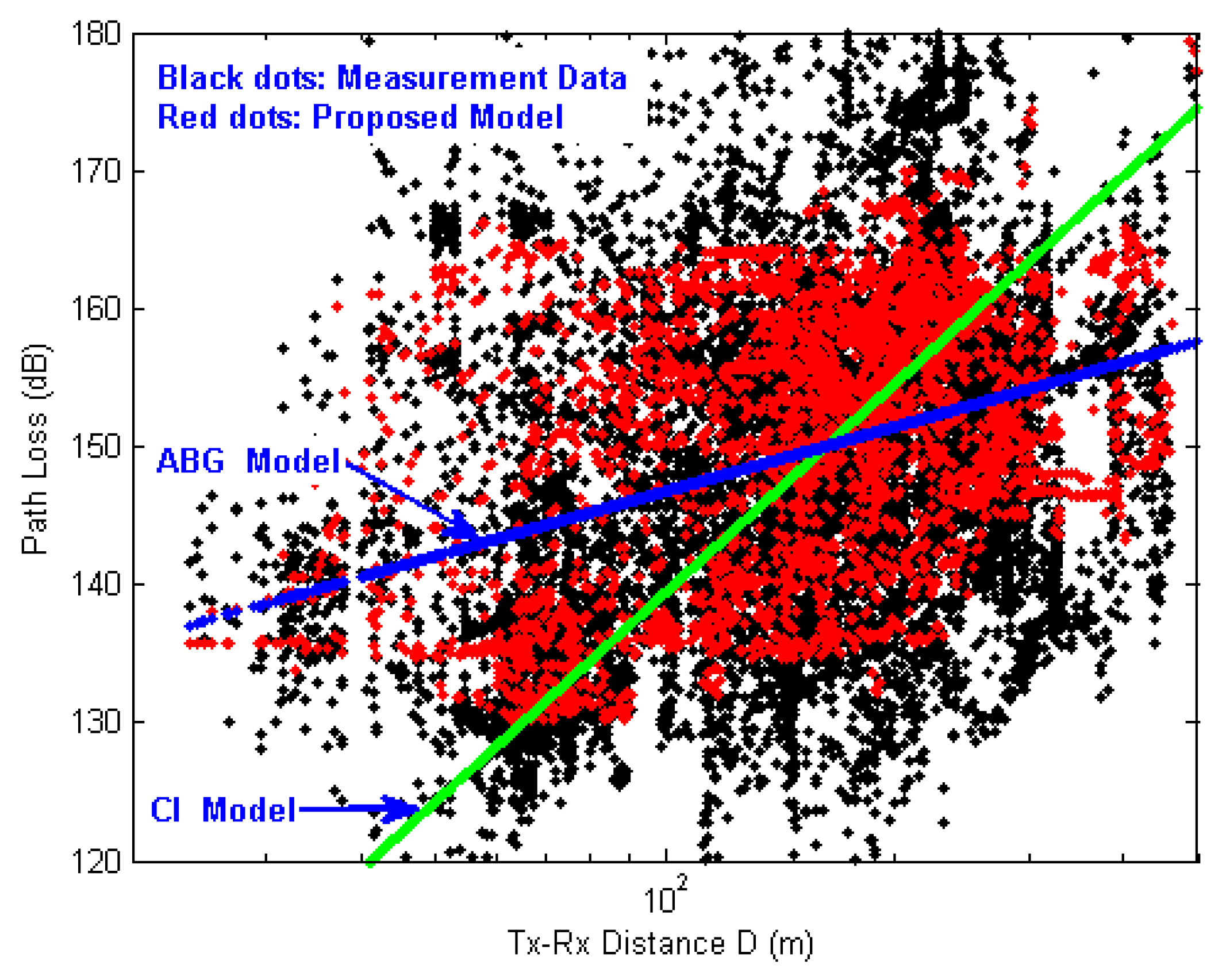
The Walfisch–Ikegami model computes the path loss by considering both LOS and NLOS conditions. The path loss in decibels is given by

$$P{L}^{WI}=L_{FS}+L_{rts}+L_{msd}$$

(1)

where $L_{FS}$ is the free space path loss, $L_{rts}$ is the roof-top-to-street diffraction and scatter loss, and $L_{msd}$ is the multiscreen diffraction loss [16,17]. These loss terms are all functions of the carrier frequency. In addition, they relate to some geometric parameters. For instance, $L_{FS}$ relates to the range between the transmitter (Tx) and receiver (Rx) pair; $L_{rts}$ relates to the average street width, the road orientation angle, and the average building height; and $L_{msd}$ relates to the average building separation, the height from the average building level to the Tx antenna, and a factor associated with diffraction loss. Note that the operating frequency for the Walfisch–Ikegami model ranges from 800 MHz to 2 GHz, although most of the 5G frequency bands are out of this range.

2.2. ABG Model

The ABG model is a simple extension to the alpha–beta (AB) model used in the 3rd Generation Partnership Project (3GPP) by adding a frequency-dependent parameter [5]. It is also one of the standard 3GPP models and is currently widely used in 5G applications [6]. The ABG model can be expressed as [5]:

$$P{L}^{ABG}=10\alpha {\log }_{10}R+\beta +10\gamma {\log }_{10}{f}_c$$

(2)

where $\alpha$ is the path loss exponent, $\beta$ is an offset term, and $\gamma$ represents the dependence of path loss on log-frequency. The optimal model parameters are typically achieved by performing linear regression with the measurement data [18].

2.3. CI Model

The CI free-space reference distance model with a 1 m reference distance is given by [5]:

$$P{L}^{CI}=L_{FS}\left(f_c,d_0\right)+10\alpha {\log }_{10}\left(R/d_0\right)$$

(3)

where $d_0$ is the close-in free-space reference distance, and $L_{FS}\left(f_c,d_0\right)$ is the free-space path loss in decibels at the carrier frequency $f_c$ and at a Tx–Rx separation distance of $d_0$. Additionally, the optimal model parameters are typically estimated by performing linear regression with measurement data [18].

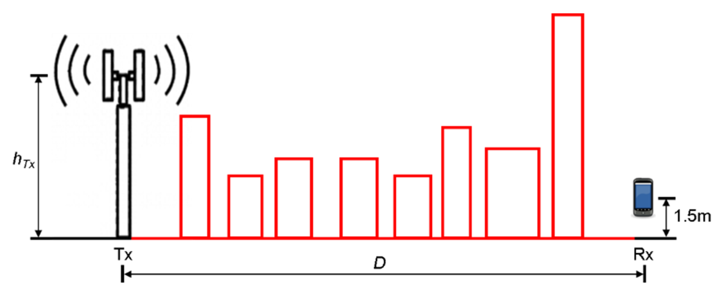
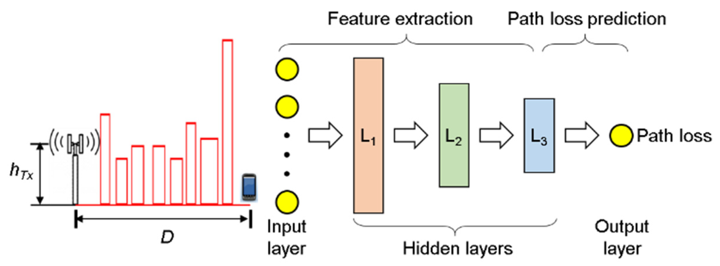
3. Problem Formulation and the Proposed Path Loss Model

In urban environments, the direct connection line between the Tx and Rx is very likely to be blocked by buildings. Figure 2 shows the conceptual overview of the Tx–Rx pair and the path profile along the direct connection line, where $h_{Tx}$ is the Tx height and $D$ is the horizontal distance. The obstruction of buildings results in excessive path loss, in addition to free space propagation. Therefore, this paper incorporates the path profile in path loss modeling.

The proposed model combines LOS and NLOS propagation scenarios. For LOS cases, where the radiation from the Tx is not blocked by buildings, the path loss is determined using the log-distance path loss model (2). For NLOS cases, this paper assumed that the excessive path loss in addition to the free space propagation is caused by the obstruction of buildings. Figure 3 shows the proposed deep-learning-based path loss model. The input data include the Tx height, $h_{Tx}$, the distance between the Tx–Rx pair, $D$, and the path profile. Assuming the cell radius is $Q$, the path profile is represented as a vector of length $Q$, with a sample distance of 1 m. The values in the profile vector stand for the building height along the path. As a result, the length of the input layer for the neural network is $Q+2$. Note that $D\le Q$, given that the Rx is within the coverage of the Tx. In the output layer, the proposed model requires only one neuron, which is used to predict the path loss. In between the input and output layers, three hidden layers, namely, L1, L2, and L3, are used to extract essential features that cause path loss.

Given the kth Tx–Rx pair, the input to the proposed deep neural network is represented as:

$$x_k={\left[\begin{array}{cccccc}{h}_{Tx,k}& D_k& q_{1,k}& q_{2,k}& \cdots & q_{Q,k}\end{array}\right]}^T$$

(4)

where $q_{i,k}$, for $1\le i\le Q$, is the building height of the kth path profile. The input should be normalized before being fed into the network because normalization has been proven to be able to accelerate the training process and improve the performance of neural networks [19]. The normalized inputs are denoted as ${\tilde{x}}_k$ and $\left({\theta }_1,b_1\right)$, $\left({\theta }_2,b_2\right)$, and $\left({\theta }_3,b_3\right)$ as the weights to be optimized at the hidden layers ${\mathrm{L}}_1$, ${\mathrm{L}}_2$ and ${\mathrm{L}}_3$, respectively. The dimensions of ${\theta }_i$ and $b_i$, for $i=1, 2, 3$, are the hyper-parameters and can be denoted as $N_i\times N_{i-1}$ and $N_i\times 1$, respectively. Note that $N_0$ is the length of the input vector, i.e., $Q+2$, and $N_1$, $N_2$ and $N_3$ are typically tuned manually by trial and error.

The features extracted by the three hidden layers can be expressed in a vector form as:

$$F_k\left(\Theta ,{\rm B}\right)={\phi }_3\left({\theta }_3{\phi }_2\left({\theta }_2{\phi }_1\left({\theta }_1{\tilde{x}}_k+b_1\right)+b_2\right)+b_3\right)$$

(5)

where $\Theta =\left({\theta }_1,{\theta }_2,{\theta }_3\right)$, ${\rm B}=\left(b_1,b_2,b_3\right)$, and ${\phi }_1$, ${\phi }_2$ and ${\phi }_3$ are the activation functions for the hidden layers. In this study, the rectified linear Unit (ReLU) activation function was adopted. Subsequently, the extracted features were used to predict the path loss based on non-linear regression. The resulting path loss, ${\widehat{y}}_k$, is given by:

$${\widehat{y}}_k\left(\Theta ,{\rm B},\mathsf{\vartheta },b\right)=\varphi \left(\mathsf{\vartheta }{F}_k\left(\Theta ,{\rm B}\right)+b\right)$$

(6)

where $\mathsf{\vartheta }$ is a row vector, $b$ is a scaler, and $\varphi$ is the sigmoid activation function. Both $\mathsf{\vartheta }$ and $b$ are also the network weights to be optimized. A training dataset of inputs is used to find the optimal weights in a supervised learning manner. The goal of optimization is to minimize the error provided by the mean squared error (MSE) function between the network output and the ground truth in the training dataset. The MSE function is given by:

$$J\left(\Theta ,{\rm B},\mathsf{\vartheta },b\right)=\frac{1}{M}{\displaystyle \sum }_{k=1}^M{\left({\widehat{y}}_k\left(\Theta ,{\rm B},\mathsf{\vartheta },b\right)-y_k\right)}^2$$

(7)

where $y_k$ is the path loss in the training dataset and $M$ is the total number of recorders. Minimizing the above cost function can be performed iteratively with the use of the error backpropagation algorithm [20]. In this study, the well-known Adam optimizer was adopted. In addition, mini-batch training was used to compute the gradient of the cost function with respect to the weights. To combat overfitting, dropout layers were also imposed.

Table 1. Hyper-parameters of the deep neural network in the proposed path loss modeling.

Category	Value
Input length	502
Output length	1
Number of hidden layers	3
Number of hidden neurons	502, 128, 8
Dropout rate	0.18
Batch size	128
Optimizer	Adam
Loss function	MSE
Activation function for feature extraction (${\phi }_i$)	ReLU
Activation function for path loss regression ($\varphi$)	Sigmoid

summarizes the hyper-parameters of the proposed path loss model. The purpose of this study is to predict path loss in urban environments; therefore, the cell radius, $Q$, was assumed to be 500 m. By trial and error, the numbers of neurons in the hidden layers were selected as $N_1=502$, $N_2=128$ and $N_3=8$.

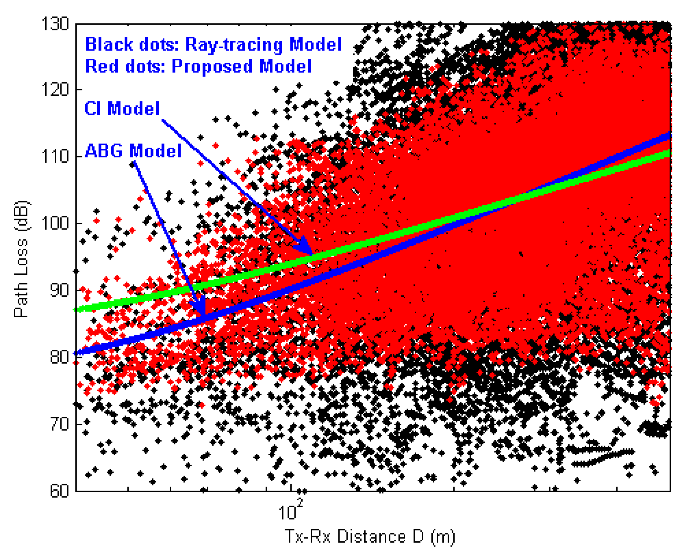
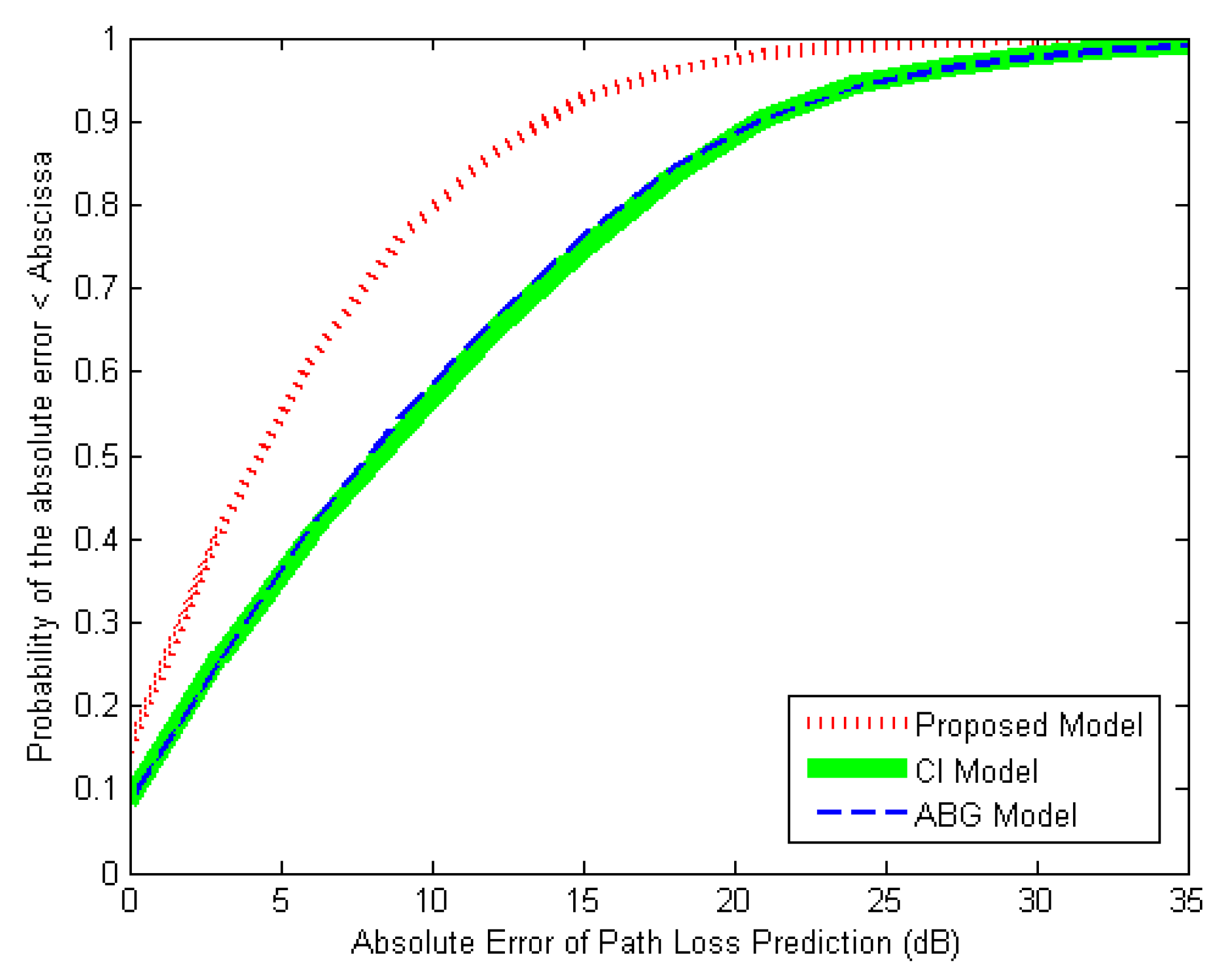
4. Analysis of Simulation Results

A software package, SignalPro^®, by EDX Wireless, Inc., was used to conduct the simulations. It provides a set of simulation tools for wireless communication systems. To facilitate simulations with site-specific geographic information, SignalPro^® supports the import of digital maps. In this study, a 3D map of urban Taipei City was imported to the software package. Figure 4 shows the top view of the simulation environment, which covered an area of 900 × 900 m². The polygons in the figure represent buildings with different heights. The means and standard deviations of building heights were 15.7 m and 8.7 m, respectively. The maximum and minimum building heights were 46 m and 4 m, respectively. Seven base stations with omnidirectional antennae were deployed and are designated by encircled crosses (⨁) in Figure 4. The center of the simulation environment was latitude 25.057457° N and longitude 121.534808° E. Readers can use Google Maps or OpenStreetMap to see more details about the regional information.

In the simulations, the effective isotropic radiated power and the height of the base stations were set to 50 dBm and 30 m, respectively. Receivers with a height of 1.5 m were placed on the roads. Distances between the Tx and Rx pairs ranged from 10 m to 500 m. The ray-tracing model was applied for the path loss calculations at the 3.5 GHz frequency band. As a result, the received power levels at all the Rx locations were recorded.

At the cost of high computational complexity, the performance of the ray-tracing model was satisfactory when compared to the field measurements [21,22]. In this work, the simulation results using the ray-tracing model were taken as the ground truth for the path loss predictions. In the simulations, 22,198 records were collected, where each record contained the receiving power and the path profile of the specific Tx–Rx pair. All the records were partitioned into training and test datasets, with an 80/20 split.

Using the test dataset, Figure 5 shows the prediction performance of the proposed path loss model and the conventional models, i.e., the ABG model and the CI model. Note that the Walfisch–Ikegami model is excluded here because the operation frequency of 3.5 GHz is out of its frequency range. In the figure, black dots are the ground-truth values, whereas red dots are the predicted values by using the proposed model. The conventional models exhibited good matches with the mean values of path loss, while the variations between the predictions and the ground-truth values are large.

Defining prediction error as the difference between the predicted value and the ground-truth value, i.e., $e_i={\widehat{y}}_i-y_i, 1\le i\le M$,

Table 2. Path loss prediction error in simulations.

	Mean Error (dB)	Standard Deviation (dB)
ABG model	0.05	13.84
CI model	0.15	13.97
Proposed model	0.04	9.13
Improvement over the ABG model	-	4.71 (34%)
Improvement over the CI model	-	4.84 (34%)

shows the statistics of the prediction errors. In terms of mean error, all the models showed good performance with only slight variances. In terms of the standard deviation, however, the proposed model outperformed the ABG and the CI models by reductions of about 4.71 dB and 4.84 dB, respectively. Furthermore, Figure 6 shows the cumulative distribution of the absolute error of path loss prediction, $\left|e_i\right|$. The proposed model outperformed the conventional models. At the 67th percentile, it reduced the error by about 41.6% from 12.29 dB to 7.17 dB when compared to the ABG model, and reduced it by about 43.6% from 12.71 dB to 7.17 dB when compared to the CI model.

5. Explainability of the Proposed Model

To obtain insight into the internal mechanism of the proposed deep-learning-based path loss model, particular inputs were selected to explore the behavior of the deep neural network. Specifically, eight relevant features were considered, as follows:

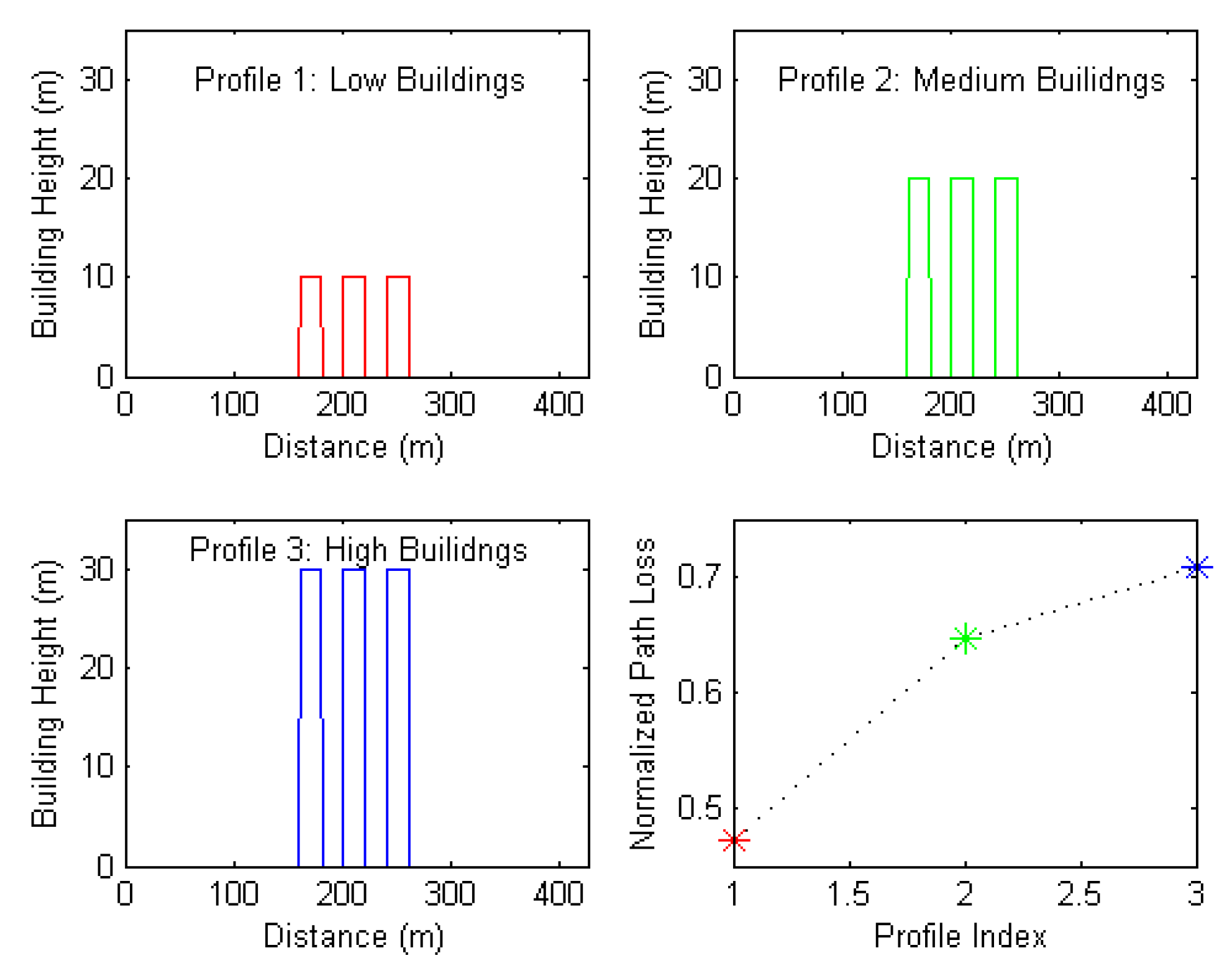
• Mean value of building height: the obstruction of buildings results in propagation loss; therefore, this feature is the arithmetic mean of building heights along the profile. Figure 7 shows three selected path profiles with low, medium, and high values of this feature. These profiles were inputted into the network and their corresponding outputs were reordered. The subfigure in the bottom right of Figure 7 shows the relationship between the path losses and the path profiles. The x-axis in the subfigure is the index of the path profile, and the y-axis is the output of the proposed deep learning model, which is a normalized path loss. This subfigure can be interpreted as the mean value of building height being relevant to outcomes of the proposed path loss model. Note that although the three classes, namely, low, medium and high, may not be sufficient to derive the exact relationship, e.g., linear, cubic, quadratic, etc., they are sufficient to verify the relevance between the feature and the path loss.
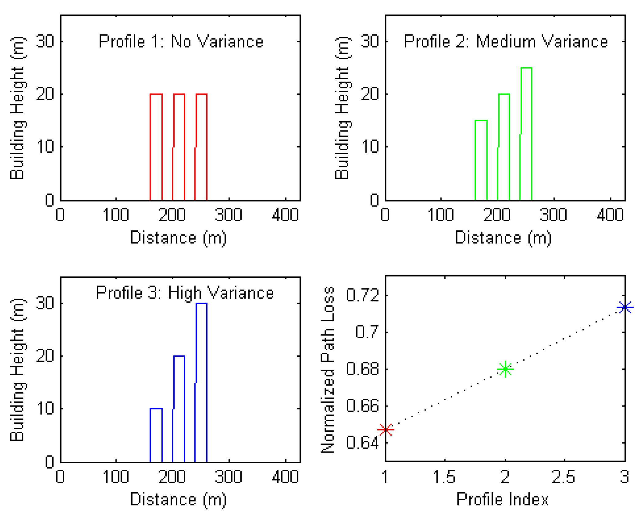
• Standard deviation of building height: this feature refers to the standard deviation of building heights along the profile. Figure 8 shows three selected path profiles with zero, medium, and high values of this feature. These three profiles were inputted into the network and their corresponding outputs were reordered. The subfigure in the bottom right of Figure 8 suggests a positive linear correlation between this feature and the predicted path loss.
• Normalized mean value of building distance: analogously to the two aforementioned features which take the statistics in the vertical axis, this feature and the subsequent one take the statistics in the horizontal axis. This feature is the arithmetic mean of the distances from the Tx to the buildings along the profile. The mean value is normalized by the Tx–Rx separation distance. Figure 9 shows three selected path profiles with buildings that are near the Tx, far from the Tx, and in between the Tx–Rx pair. These profiles were inputted into the network and their corresponding outputs were reordered. The subfigure in the bottom right of Figure 9 indicates a non-linear relationship between this feature and the predicted path loss.
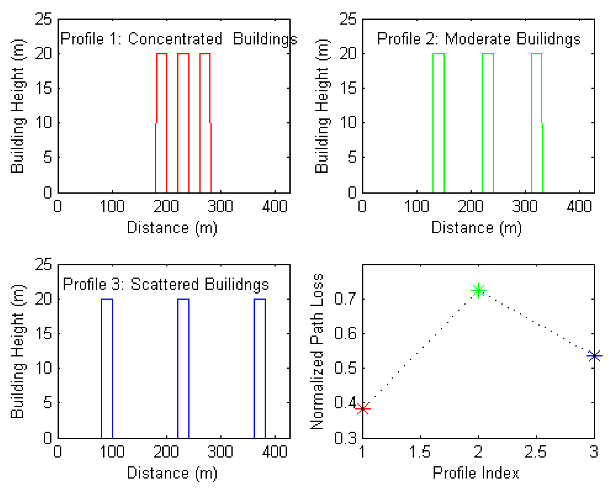
• Normalized standard deviation of building distance: this feature refers to the standard deviation of the distances from the Tx to the buildings along the profile. The standard deviation is normalized by the Tx–Rx separation distance. Figure 10 shows three selected path profiles with concentrated buildings, scattered buildings, and moderate buildings. These profiles were inputted into the network and their corresponding outputs were reordered. The subfigure in the bottom right of Figure 10 indicates a non-linear relationship between this feature and the predicted path loss.
• Building density: in addition to the above two statistics in the horizontal axis, this feature describes the percentage of buildings along the profile. Figure 11 shows three selected path profiles with low, medium, and high values of this feature. These profiles were inputted into the network and their corresponding outputs were reordered. The subfigure in the bottom right of Figure 11 shows that this feature and the predicted path loss have a positive relationship that can be approximated in a linear form.
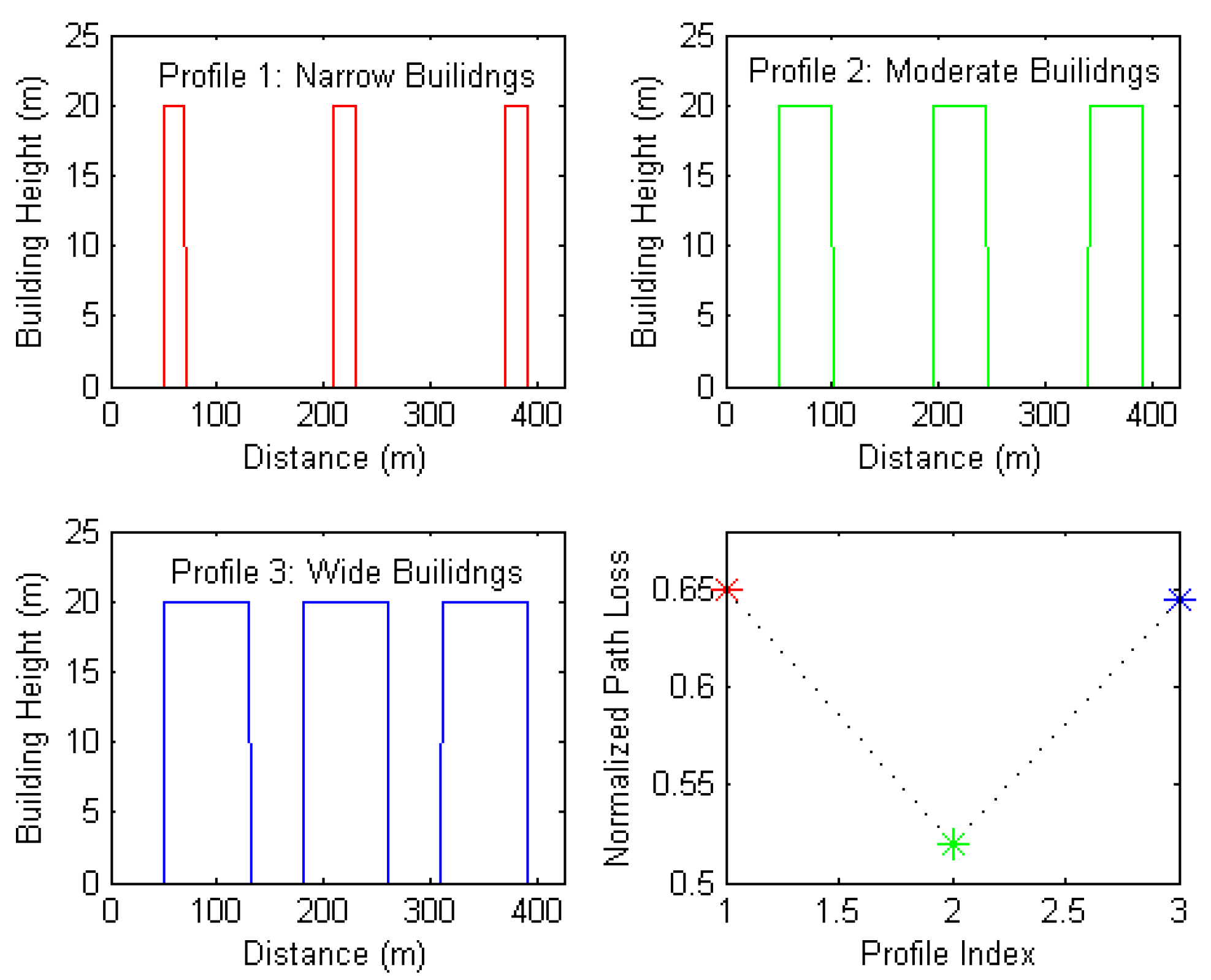
• Average building width: this feature refers to the arithmetic mean building width along the profile. It also implies the average street width. Figure 12 shows three selected path profiles with narrow buildings, wide buildings, and moderate buildings. These profiles were inputted into the network and their corresponding outputs were reordered. The subfigure in the bottom right of Figure 12 indicates a non-linear relationship between this feature and the predicted path loss
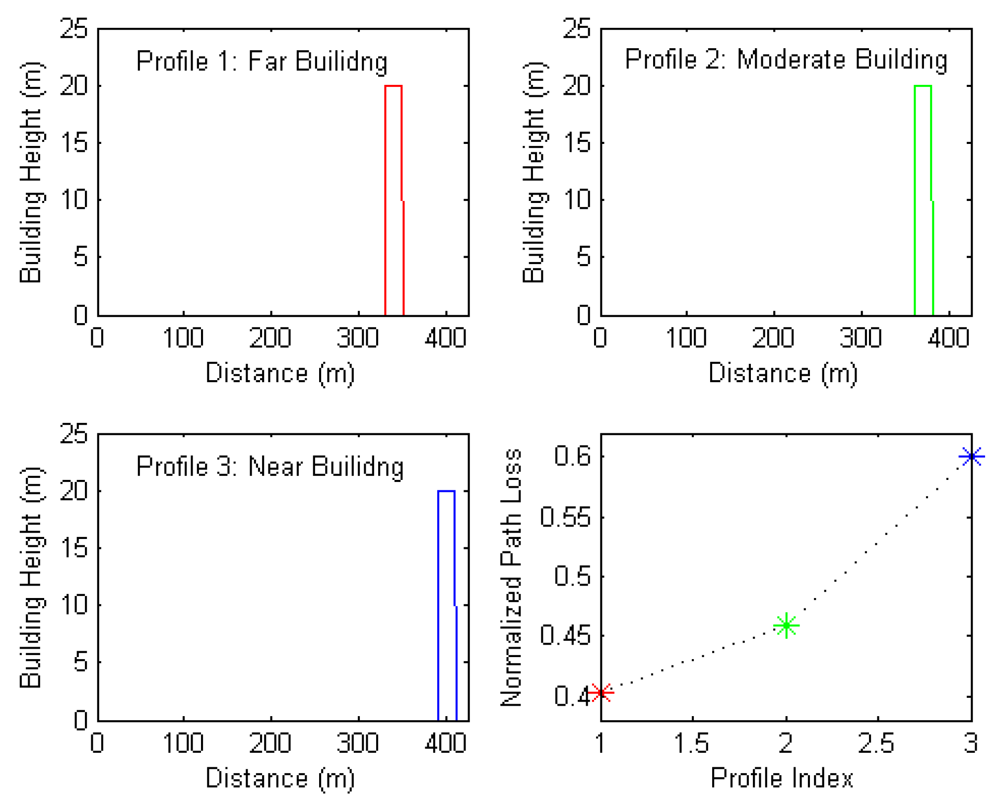
• Distance to the nearest building from the Rx: in general, the path loss tends to be high when a high building is close to the Rx. This feature refers to the distance from the Rx to the nearest building along the profile. Figure 13 shows three selected path profiles with a building far from the Rx, near the Rx, and at a moderate distance. These profiles were inputted into the network and their corresponding outputs were reordered. The subfigure in the bottom right of Figure 13 indicates that this feature is relevant to the path loss prediction.
• Height of the nearest building from the Rx: this feature is the height of the nearest building along the profile from the Rx. Figure 14 shows three selected path profiles with low, medium, and high values of this feature. These profiles were inputted into the network and their corresponding outputs were reordered. The subfigure in the bottom right of Figure 14 suggests a positive linear correlation between this feature and the predicted path loss.

To evaluate the quality and appropriateness of the explainability of the proposed deep neural network, the aforementioned features were used to model the path loss based on the approach of linear regression. For single-frequency scenarios, the log-frequency term in Equation (2) can be merged into the left-hand side. Here, the coefficient $\gamma$ in Equation (2) is set to two. The path loss for the kth Tx–Rx pair is given by

$$P{L}_k^{XAI}=10\alpha lo{g}_{10}{R}_k+\beta +{\displaystyle \sum }_{i=1}^8{u}_i{z}_{i,k}+{\displaystyle \sum }_{i=1}^8{v}_i{z}_{i,k}^2$$

(8)

where $z_{i,k}$, for $1\le i\le 8$, stands for the eight aforementioned features. $\alpha$, $\beta$, $u_i$, and $v_i$ are model parameters to be optimized. Although some features seem to be linearly correlated with the path loss prediction, their quadratic forms are also considered in Equation (8), because they do no harm to the path loss model. To achieve the optimal model parameters based on the least-square regression, Equation (8) can be expressed in matrix form as:

$$Y=\Gamma \mathsf{\omega }$$

(9)

where:

$$Y={\left[\begin{array}{cccc}{y}_1& y_2& \cdots & y_M\end{array}\right]}^T$$

(10)

$${\rm Z}=\left[\begin{array}{cccccccccc}10lo{g}_{10}{R}_1& 1& z_{1,1}& z_{2,1}& \cdots & z_{8,1}& z_{1,1}^2& z_{21}^2& \cdots & z_{8,1}^2\\ 10lo{g}_{10}{R}_2& 1& z_{1,2}& z_{2,2}& \cdots & z_{8,2}& z_{1,2}^2& z_{2,2}^2& \cdots & z_{8,2}^2\\ ⋮& ⋮& ⋮& ⋮& \ddots & ⋮& ⋮& ⋮& \ddots & ⋮\\ 10lo{g}_{10}{R}_M& 1& z_{1,M}& z_{2,M}& \cdots & z_{8,M}& z_{1,M}^2& z_{2,M}^2& \cdots & z_{8,M}^2\end{array}\right]$$

(11)

$$\mathsf{\omega }={\left[\begin{array}{cccccccccc}\alpha & \beta & u_1& u_2& \cdots & u_8& v_1& v_2& \cdots & v_8\end{array}\right]}^T$$

(12)

As a result, the optimal parameter that minimizes the fitting error is given by [6]:

$${\mathsf{\omega }}_{\mathrm{OPT}}={\left({{\rm Z}}^T{\rm Z}\right)}^{-1}{{\rm Z}}^{T}Y$$

(13)

Additionally, the predicted path loss can be expressed as:

$${\widehat{y}}_k=z_k{\mathsf{\omega }}_{\mathrm{OPT}}$$

(14)

where $z_k=\left[\begin{array}{cccccccccc}10lo{g}_{10}{R}_k& 1& z_{1,k}& z_{2,k}& \cdots & z_{8,k}& z_{1,k}^2& z_{2,k}^2& \cdots & z_{8,k}^2\end{array}\right]$.

Figure 15 shows the prediction performance of the proposed deep learning model and the explanatory model. The graphics are plotted in the sense of time series. The blue curve is the outcome of the deep learning model, whereas the red dots are the values predicted using the explanatory model. To quantify the accuracy of the explanatory model, the accuracy metric is defined as the correlation coefficient between the explanatory model and the proposed deep learning model. ${\mu }_{\tilde{y}}$ and ${\mu }_{\widehat{y}}$ are denoted as the mean values of the path loss predictions by using the explanatory model and the proposed deep learning model, respectively. Additionally, ${\sigma }_{\tilde{y}}$ and ${\sigma }_{\widehat{y}}$ are denoted as the standard deviation of the path loss predictions by using the explanatory model and the proposed deep learning model, respectively. The accuracy metric is defined as:

$$\rho =\frac{E\left[\left(\tilde{y}-{\mu }_{\tilde{y}}\right)\left(\widehat{y}-{\mu }_{\widehat{y}}\right)\right]}{{\sigma }_{\tilde{y}}{\sigma }_{\widehat{y}}}$$

(15)

where $E\left[·\right]$ is the expectation operation. As a result, the accuracy reaches 72%. Note that this accuracy metric can be also considered as the transparency of the proposed deep learning model, which is a black box in nature.

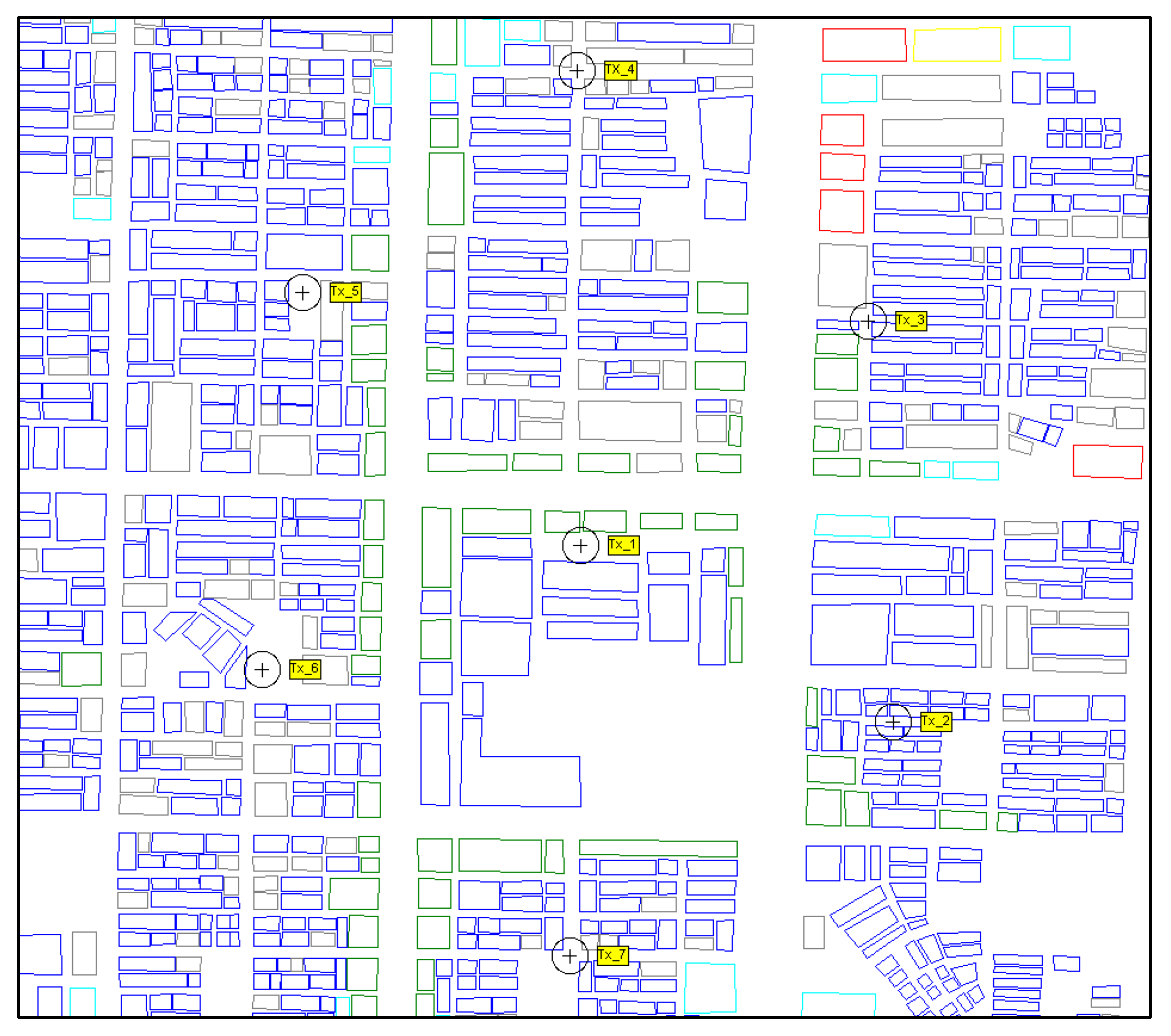
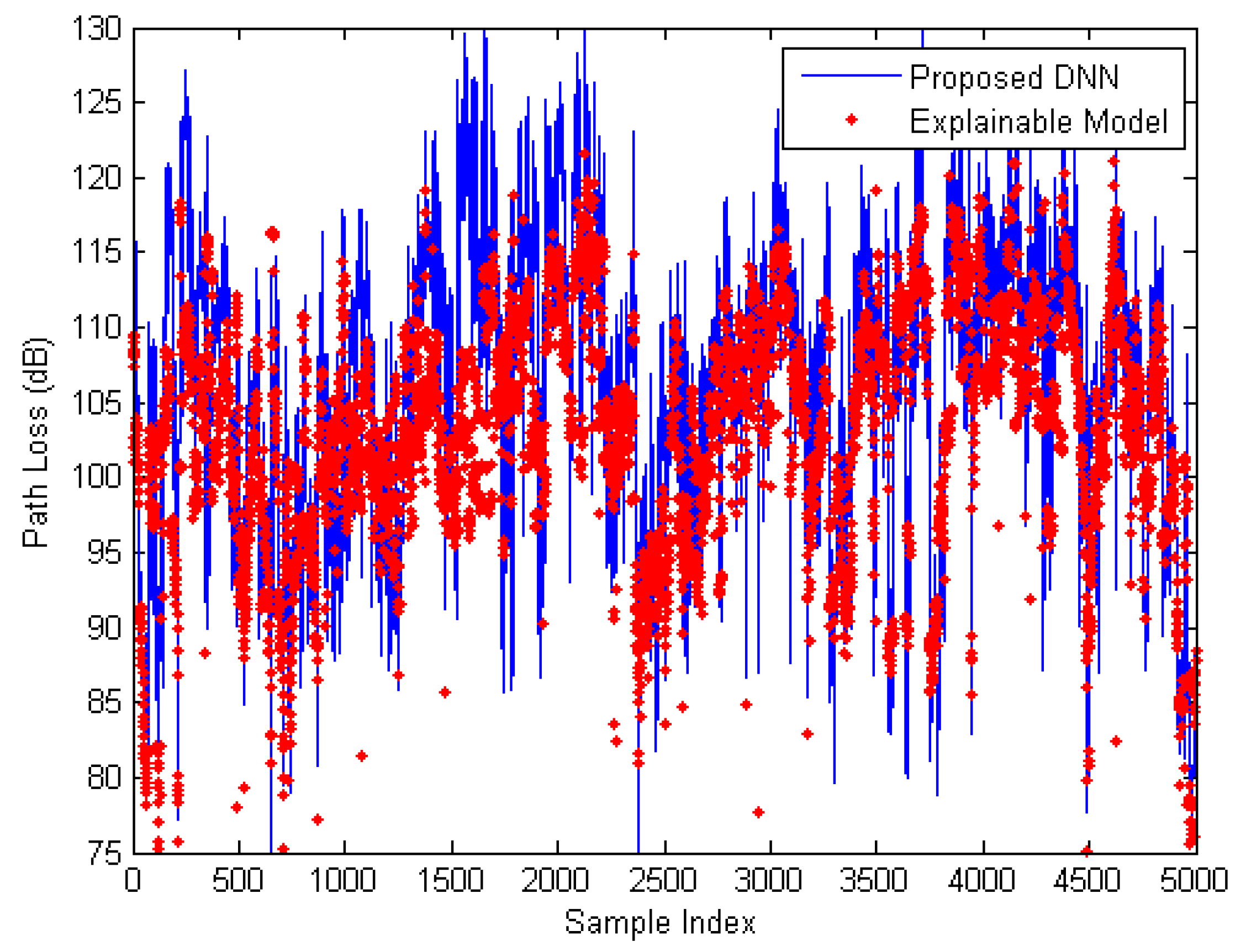
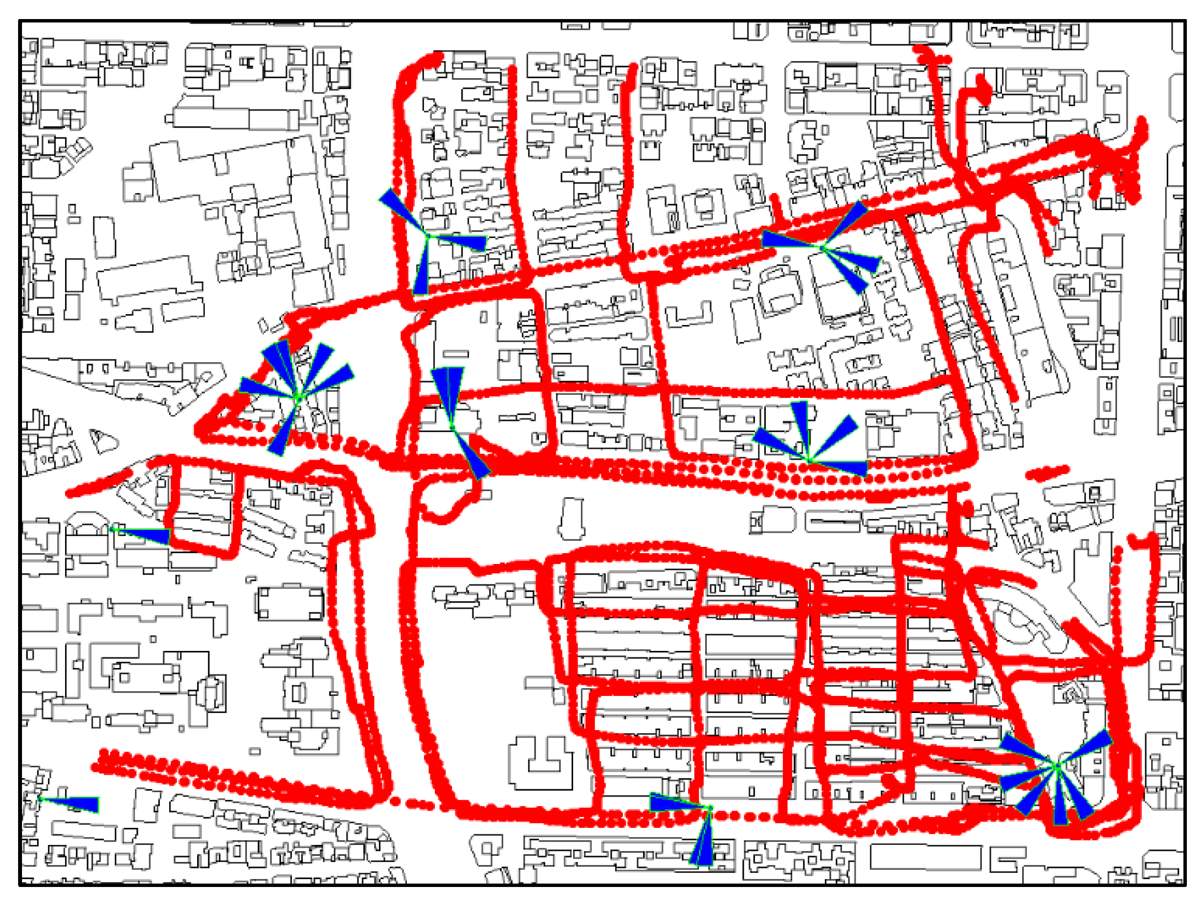
6. Verifying Performance using 5G NR Measurement Data

The proposed deep-learning-based path loss model was further applied to a real non-standalone 5G NR system in the urban environment of Taipei City. As shown in Figure 16, the measurement environment was located at latitude 25.044773° N and longitude 121.539456° E, and covered an area of 1 × 1 km². Nine base stations operating in the 2.1 GHz frequency band were included in the measurement area. Measurement equipment was placed in a vehicle driving along selected routes. The measurement reports include the reference symbol received power (RSRP), E-UTRAN cell identity (ECI), and the vehicle’s GNSS coordinates. Then, the path losses between the Tx–Rx pairs were calculated according to the link budgets.

There were 16,359 records collected during the measurement tasks. Figure 17 shows the prediction performance of the proposed path loss model and the conventional models. The black dots are the measurements, whereas the red dots are the values predicted using the proposed model. The blue and the green curves represent the predictions using the ABG and CI models, respectively.

Table 3. Path loss prediction error in measurements.

	Mean Error (dB)	Standard Deviation (dB)
ABG model	0.00	11.11
CI model	−0.84	13.69
Proposed model	0.42	7.70
Improvement over the ABG model	-	3.41 (30%)
Improvement over the CI model	-	5.99 (43%)

shows the statistics of prediction error resulting from the measurements. The conventional models and the proposed model show good matches in terms of the mean prediction error. In terms of the standard deviation, however, the proposed model outperformed the ABG model and the CI model by reducing it by about 3.41 dB and 5.99 dB, respectively. Furthermore, Figure 18 shows the cumulative distribution of the absolute error of path loss prediction. The proposed model outperformed the conventional models. At the 67th percentile, it reduced the error by about 32.1%, from 9.30 dB to 6.31 dB, when compared to the ABG model, and by about 42.3%, from 10.95 dB to 6.31 dB, when compared to the CI model. Additionally, the explanatory model was used to evaluate the explainability of the proposed deep learning model in the realistic 5G environment. The measurement data show that the accuracy $\rho$ reached 63%.

7. Conclusions

By applying deep learning methodology, this paper has presented a path loss model based on a profile along the direct propagation path between Tx–Rx pairs in urban environments for 5G cellular communication systems. The neural network of the proposed model extracts important features and then predicts the path loss based upon them. Simulation results showed that the proposed model outperforms conventional models. The standard deviation of prediction error was reduced by 34% when compared to the conventional models. In addition to pursuing the prediction performance empowered by the nonlinear mapping of the deep learning method, this paper has also explored the internal mechanism of the neural network. Eight explainable features were tested and used to predict the path loss, based on a linear regression approach. The simulation results showed that the accuracy of the explainable model reached 72%. Furthermore, the proposed deep learning model was also evaluated in a non-standalone 5G NR network in urban Taipei City. The measurements show that the standard deviation of prediction error was reduced by 30–43% when compared to the conventional models, and that the accuracy of the explanatory model reached 63% in the realistic 5G network.

References

1. Vannithamby, R.; Talwar, S. Towards 5G: Applications, Requirements and Candidate Technologies; Wiley: Hoboken, NJ, USA, 2017. [Google Scholar]
2. Popoola, S.I.; Atayero, A.A.; Arausi, O.D.; Matthews, V.O. Path loss Dataset for Modeling Radio Wave Propagation in Smart Campus Environment. ELSEVIER Data Brief 2018, 17, 1062–1073. [Google Scholar] [CrossRef]
3. Salous, S.; Lee, J.; Kim, M.D.; Sasaki, M.; Yamada, W.; Raimundo, X.; Cheema, A.A. Radio Propagation Measurements and Modeling for Standardization of the Site General Path Loss Model in International Telecommunications Union Recommendations for 5G Wireless Networks. Radio Sci. 2020, 55, e2019RS006924. [Google Scholar] [CrossRef] [Green Version]
4. Shabbira, N.; Kütta, L.; Alamb, M.M.; Roosipuub, P.; Jawadc, M.; Qureshic, M.B.; Ansarid, A.R.; Nawaze, R. Vision Towards 5G: Comparison of Radio Propagation Models for Licensed and Unlicensed Indoor Femtocell Sensor Networks. ELSEVIER Phys. Commun. 2021, 47, 101371. [Google Scholar] [CrossRef]
5. Sun, S.; Rappaport, T.S.; Thomas, T.A.; Ghosh, A.; Nguyen, H.C.; Kovács, I.Z.; Rodriguez, I.; Koymen, O.; Partyka, A. Investigation of Prediction Accuracy, Sensitivity, and Parameter Stability of Large-Scale Propagation Path Loss Models for 5G Wireless Communications. IEEE Trans. Veh. Technol. 2016, 65, 2843–2860. [Google Scholar] [CrossRef]
6. Casillas-Perez, D.; Camacho-Gómez, C.; Jiménez-Fernandez, S.; Portilla-Figueras, J.A.; Salcedo-Sanz, S. Weighted ABG: A General Framework for Optimal Combination of ABG Path-Loss Propagation Models. IEEE Access 2020, 8, 101758–101769. [Google Scholar] [CrossRef]
7. Samimi, M.K.; Rappaport, T.S.; MacCartney, G.R., Jr. Probabilistic Omnidirectional Path Loss Models for Millimeter-Wave Outdoor Communications. IEEE Wirel. Commun. Lett. 2015, 4, 357–360. [Google Scholar] [CrossRef]
8. Zhang, Y.; Wen, J.; Yang, G.; He, Z.; Wang, J. Path Loss Prediction Based on Machine Learning: Principle, Method, and Data Expansion. Appl. Sci. 2019, 9, 1908. [Google Scholar] [CrossRef] [Green Version]
9. Moraitis, M.; Tsipi, L.; Vouyioukas, D. Machine Learning-Based Methods for Path Loss Prediction in Urban Environment for LTE Networks. In Proceedings of the IEEE International Conference on Wireless and Mobile Computing, Networking and Communications (WiMob), Thessaloniki, Greece, 12–14 October 2020. [Google Scholar]
10. Thrane, J.; Zibar, D.; Christiansen, H.L. Model-Aided Deep Learning Method for Path Loss Prediction in Mobile Communication Systems at 2.6 GHz. IEEE Access 2020, 8, 7925–7936. [Google Scholar] [CrossRef]
11. Ates, H.F.; Hashir, S.M.; Baykas, T.; Gunturk, B.K. Path Loss Exponent and Shadowing Factor Prediction from Satellite Images using Deep Learning. IEEE Access 2019, 7, 101366–101375. [Google Scholar] [CrossRef]
12. Cheng, H.; Ma, S.; Lee, H. CNN-Based mmWave Path Loss Modeling for Fixed Wireless Access in Suburban Scenarios. IEEE Antennas Propag. Lett. 2020, 19, 1694–1698. [Google Scholar] [CrossRef]
13. Ahmadien, O.; Ates, H.F.; Baykas, T.; Gunturk, B.K. Predicting Path Loss Distribution of an Area from Satellite Images Using Deep Learning. IEEE Access 2020, 8, 64982–64991. [Google Scholar] [CrossRef]
14. Adadi, A.; Berrada, M. Peeking Inside the Black-Box: A Survey on Explainable Artificial Intelligence (XAI). IEEE Access 2018, 6, 52138–52160. [Google Scholar] [CrossRef]
15. Guo, W. Explainable Artificial Intelligence for 6G: Improving Trust between Human and Machine. IEEE Commun. Mag. 2020, 58, 39–45. [Google Scholar] [CrossRef]
16. Saunders, S.R. Antennas and Propagation for Wireless Communication Systems; Wiley: Hoboken, NJ, USA, 1999. [Google Scholar]
17. Har, D.; Watson, A.M.; Chadney, A.G. Comment on Diffraction Loss of Rooftop-to-Street in COST 231-Walfisch–Ikegami Model, IEEE Trans. Veh. Technol. 1999, 48, 1451–1452. [Google Scholar] [CrossRef]
18. Sun, S.; Rappaport, T.S.; Rangan, S.; Thomas, T.A.; Ghosh, A.; Kovacs, I.Z.; Rodriguez, I.; Koymen, O.; Partyka, A.; Jarvelainen, J. Propagation Path Loss Models for 5G Urban Micro- and Macro-Cellular Scenarios. In Proceedings of the IEEE Vehicular Technology Conference, Nanjing, China, 15–18 May 2016. [Google Scholar]
19. Hochreiter, S.; Schmidhuber, J. Long short-term memory. Neural Comput. 1997, 9, 1735–1780. [Google Scholar] [CrossRef] [PubMed]
20. Siddique, M.N.H.; Tokhi, M.O. Training neural networks: Backpropagation vs. genetic algorithms. In Proceedings of the International Joint Conference on Neural Networks, Washington, DC, USA, 15–19 July 2001. [Google Scholar]
21. Ai, B.; Guan, K.; He, R.; Li, J.; Li, G.; He, D.; Zhong, Z.; Huq, K.M.S. On Indoor Millimeter Wave Massive MIMO Channels: Measurement and Simulation. IEEE J. Sel. Areas Commun. 2017, 35, 1678–1690. [Google Scholar] [CrossRef]
22. Zhu, M.; Singh, A.; Tufvesson, F. Measurement Based Ray Launching for Analysis of Outdoor Propagation. In Proceedings of the 6th European Conference Antennas and Propagation (EUCAP), Prague, Czech Republic, 26–30 March 2012. [Google Scholar]
Figure 1. Conceptual graphic of the proposed solution.
Applsci 11 06690 g001
Figure 2. Illustration of the Tx–Rx pair and its path profile.
Applsci 11 06690 g002
Figure 3. The network architecture of the proposed deep-learning-based path loss modeling.
Applsci 11 06690 g003
Figure 4. Top view of the simulation environment which covers an area of 900 m × 900 m. Buildings are represented by colored polygons. The base stations with omnidirectional antennae are designated by the encircled crosses (⨁).
Applsci 11 06690 g004
Figure 5. Prediction performance of the proposed path loss model and the conventional models in simulations.
Applsci 11 06690 g005
Figure 6. The cumulative distribution of the absolute error of path loss predictions in simulations.
Applsci 11 06690 g006
Figure 7. The relevance of the mean value of building height to the proposed path loss model.
Applsci 11 06690 g007
Figure 8. The relevance of the standard deviation of building height to the proposed path loss model.
Applsci 11 06690 g008
Figure 9. The relevance of the normalized mean value of building distance to the proposed path loss model.
Applsci 11 06690 g009
Figure 10. The relevance of the normalized standard deviation of building distance to the proposed path loss model.
Applsci 11 06690 g010
Figure 11. The relevance of the density of buildings to the proposed path loss model.
Applsci 11 06690 g011
Figure 12. The relevance of the average building width (or average street width) to the proposed path loss model.
Applsci 11 06690 g012
Figure 13. The relevance of the distance to the nearest building from the Rx to the proposed path loss model.
Applsci 11 06690 g013
Figure 14. The relevance of the height to the nearest building from the Rx to the proposed path loss model.
Applsci 11 06690 g014
Figure 15. Prediction performance of the proposed deep learning model and the explanatory model.
Applsci 11 06690 g015
Figure 16. Top view of the measurement environment, where the polygons, triangles, and red dots represent the buildings, cell sectors, and receivers, respectively.
Applsci 11 06690 g016
Figure 17. Prediction performance of the proposed path loss model and the conventional models in measurements.
Applsci 11 06690 g017
Figure 18. The cumulative distribution of the absolute error of path loss prediction in simulations.
Applsci 11 06690 g018