A Co-Rotational Meshfree Method for the Geometrically Nonlinear Analysis of Structures

Abstract

This paper presents a co-rotational beam formulation, which is used for geometric nonlinear analysis with the differential reproducing kernel (DRK) approximation collocation method. The present formulation, based on the Timoshenko beam hypothesis, is capable of effectively solving geometrically nonlinear problems such as large deformation, postbuckling, lateral buckling, and snap-through problems. The kinematics have been constructed with the concept of co-rotational formulation adopted in the finite element method (FEM). A meshfree method based on the differential reproducing kernel (DRK) approximation collocation method, combined with the Newton–Raphson method, is employed to solve the strong forms of the geometrically nonlinear problems. The DRK method takes full advantage of the meshfree method. Moreover, only a scattered set of nodal points is necessary for the discretization. No elements or mesh connectivity data are required. Therefore, DRK will be able to completely circumvent the problems of mesh dependence and mesh distortion. The effectiveness of this study and its performance are shown through several numerical applications.

1. Introduction

The geometrically nonlinear analysis of a beam structure undergoing large displacement remains a strong topic of interest, with applications in various fields such as civil engineering over the past few decades. Various formulation strategies and numerical procedures using FEM have been developed to deal with the large deformation problems [1,2,3,4,5,6,7,8,9,10,11,12,13,14,15,16,17,18,19,20,21,22]. For the large displacements and finite rotation problems of a geometrically nonlinear analysis, the description of the kinematics can be regarded as the dominant factor. The formulations used to describe the kinematics of beam structures in the literature might be divided into three categories: total Lagrangian (TL) formulation [2,5,9,11,12,15], updated Lagrangian (UL) formulation [3,7,18], and co-rotational (CR) formulation [4,8,10]. The main difference between these formulations lies in their definitions of the reference of the coordinates adopted in FEM. In the total Lagrangian formulation, the initial undeformed configuration is adopted as the reference configuration. Consequently, the system equations are defined with respect to the fixed global coordinate system through the analysis. In contrast, the updated Lagrangian formulation adopted the local coordinate system, updated with the current configuration, as the reference configuration—that is, the system equations were constructed at the current deformed beam configuration. Generally, the system equations expressed in the updated Lagrangian formulation will be simpler than the corresponding equations in the total Lagrangian formulation. However, if the displacement from the current configuration to the last equilibrium configuration is large, it will be in violation of the basic assumption and will lead to unreliable results. To circumvent this problem, the co-rotational formulation was introduced. In the co-rotational framework, there are global coordinates and co-rotational coordinates, kept fixed at the deformed beam segment during the analysis procedure. The co-rotational coordinate rotates and translates with each element but does not deform with it. Therefore, the total motions of the element can be divided into the rigid body part and the purely deformational part.

For the finite element formulation, another important issue is the choice of the primary interpolated variables. No matter which of the above formulations is adopted to describe the kinematics, most of the large deformation analyses performed with the FEM use the conventional displacement approach with the principle of virtual work or minimum potential energy [2,3,4,5]. Both displacements and rotations or rotations alone are taken as the interpolated variables in the finite element implementation. Hence, the choice of the primary interpolated variables is also an important issue in the finite element formulation. In standard finite element formulations, the stress resultants solved by the equilibrium equations, and those computed by the constitutive equations, are not equal since the differentiated quantities are, as a rule, one order less accurate than the quantity itself. When formulations based on displacement and rotation were employed, the strains had to be computed by differentiating toward the assumed kinematic field. The internal forces and moments will be evaluated by the constitutive law with the recovered strain field. However, the accuracy of the differentiated quantities may decline. In particular, employing low-order shape functions to solve the shear flexible models may yield locking problems. Therefore, the performance of the element may deteriorate rapidly while dealing with shear flexible models such as thinner beam problems. However, the numerical effect can be corrected with the aid of reduced integration. Still, the displacement–rotation-based formulations may acquire inaccurate stress fields due to recovery by the differentiation procedure, even if the displacement fields can be solved accurately. To circumvent the numerical problem, some researchers have taken strain vectors [13] or stress resultants [16] as the primary variables. For instance, Zupan and Saje [13] presented a formulation in terms of the strain vectors such that the additive interpolation has no restrictions. On the contrary, Cannarozzi and Molari [16] took the stress vectors as the only interpolated degree of freedom. In this way, the displacement can be obtained by integration of the kinematic equations. Magisano et al. [21] developed a large rotation finite element analysis of three-dimensional beams based on the Mixed Integration Point (MIP) Newton iterative scheme [22], in which the co-rotational nodal rotations defined by incremental nodal rotation vectors are interpolated for the evaluation of the nonlinear strains. In the above studies, whether the stress or strain vectors have been employed to be the interpolated variables in the finite element formulation, it still deals with the weak form based on the principle of virtual work or the principle of minimum potential energy.

As opposed to FEM, adopted to solve numerical analysis, in this study a meshfree method based on the Differential Reproducing Kernel (DRK) Approximation collocation method combined with the Newton–Raphson method was adopted to analyze geometrically nonlinear problems. The kinematics of beam structures undergoing large deformation are derived with the concepts of the co-rotational framework. It is well-known that the primary characteristic of meshfree methods is that the domain is completely discretized by a scattered set of nodal points instead of elements. However, this naturally circumvents mesh problems may result in numerical problems in FEM. Therefore, in the present scheme the solution of nonlinear equilibrium equations such as displacements, rotations, and force resultants of a beam that has undergone large deformation will be directly solved toward the strong form of the governing equations. The DRK implementation of the three-dimensional co-rotational beam formulation, leading to differentiation of the assumed kinematic field, is not necessary while evaluating strains, internal forces, and moments. This also shows that the primary interpolated variables will not be the dominant factor in the present scheme.

In the literature, meshfree methods have been used by numerous researchers [23,24,25,26,27,28,29,30,31,32,33,34]. Several meshfree methods, including collocation and finite point methods based on different approximations, have been proposed to solve the strong form problems. Aluru [28] implemented a point collocation method to solve the differential equations by reproducing kernel approximations.

Onate et al. [29] adopted weighted least squares interpolations to develop a finite point method to analyze elasticity problems. Yang et al. [30] proposed a radial basis collocation method with a strong-form generalized displacement control method to solve geometrically nonlinear problems. Most point collocation methods are based on the idea of reproducing kernel (RK)approximations. However, conventional RK methods compute the derivatives of the shape functions by differentiating toward the shape functions directly. In particular, this may lead to complex expressions and computations while computing high-order derivatives. Several methods were developed to solve the complicated problems. Wang et al. [31] employed a trivial numerical implementation of second-order smoothed gradients to develop a superconvergent gradient smoothing meshfree collocation method. Wang et al. [32], Yang et al. [33], and Yeh [34] developed the DRK method for one-dimensional and two-dimensional elasticity analysis.

In comparison with the conventional RK approximations, the DRK approximations involve the calculation of the derivatives of shape functions in the conventional RK. In the DRK approximations, the derivatives will be determined by the differential reproducing conditions instead of differentiating toward the shape functions directly in the conventional RK. In the present paper, the meshfree method based on the DRK approximations proposed by Wang et al. [32,33] and Yeh [34] is adopted to solve the geometrically nonlinear problems. In addition to the advantage of having no mesh, the DRK method also allows for easy computation of the derivative of the shape function. This characteristic enables the DRK approximations to construct system equations easily and directly from the governing equations. The aim of the present paper is to develop a three-dimensional co-rotational beam formulation with the aid of the DRK approximations combined with the Newton–Raphson method. The effectiveness of this approach and its performance are shown by numerical examples.

2. Theoretical Formulation

2.1. Basic Assumptions

The following assumptions are made in the derivation of the three-dimensional co-rotational beam formulation:

• The Timoshenko beam hypothesis is valid.
• The theory is limited to elasticity problems.
• The twist rate and unit extension of the centroid axis of the beam are uniform.
• The displacements and rotations of the beam can be large.
• The out-of-plane warping of the cross section is excluded.

2.2. Geometry and Kinematics of Three-Dimensional Beam

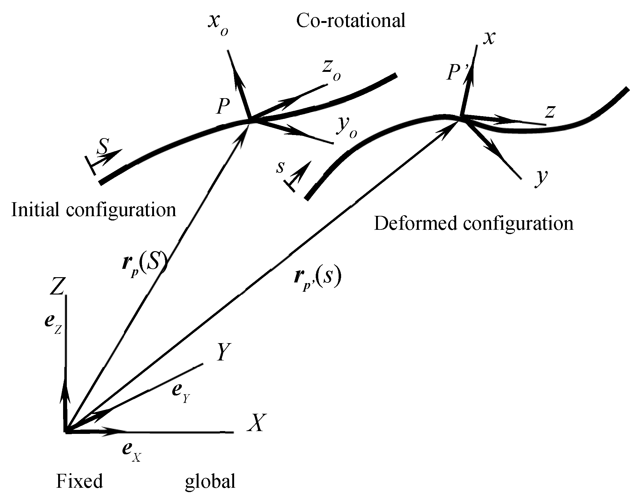
2.2.1. Coordinate System

In order to describe the geometry and kinematics of the beam in the undeformed and deformed configurations, we defined two sets of right-handed rectangular Cartesian coordinate systems:

1. Fixed global coordinates:

As shown in Figure 1, the global coordinate, which remains fixed during the entire analysis, describes the displacements, rotation, and curvature of the structure. The governing equations of the system are also constructed with respect to the global coordinates.

2. Co-rotational local rectangular Cartesian coordinates:

The DRK collocation method adopts a scattered set of nodal points to fulfill the discretization instead of the element adopted in FEM. Hence, a set of co-rotational local coordinates has to be defined, associated with the nodal points collocated on the centroidal axis of each cross section. The origin of the co-rotational local coordinate system is tied to the centroid of the cross section. The x_o and y_o axes of the co-rotational local coordinates are taken as the principal directions of the cross section. In addition, the z_o axis is selected to coincide with the normal direction of the cross section. In this way, this co-rotational local coordinate will be co-rotated with the beam undergoing large deformation.

2.2.2. Kinematics of Deformed Beam

From the kinematic assumptions made in the present paper, the deformations of the beam can be described by the displacements and rotation of the beam centroid axis. As shown in Figure 1, the position vector of an arbitrary point P on the beam centroidal axis at the undeformed and deformed configuration can be expressed as follows:

r_p(S) = X_o(S) e_X + Y_o(S) e_Y + Z_o(S) e_Z

(1)

And

r_p’ (s) = X(s) e_X + Y(s) e_Y + Z(s) e_Z,

(2)

where e_X, e_Y, and e_Z are the unit basis vector of the global coordinates; S and s are the arc length of beam centroidal axis in undeformed and deformed configuration, respectively. Moreover, X_o(S), Y_o(S), Z_o(S) and X(s), Y(s), Z(s) are the coordinate components of the position vector associated with undeformed and deformed configuration.

From the geometric relationship between the global and co-rotational local coordinates at deformed configuration, Equation (3) can be given as follows:

e_z(s) = dr(s)/ds.

(3)

The relationship between the global and co-rotational local coordinate associated with each nodal point by collocation point method on the deformed beam axis can be represented by the rotation matrix R(s):

e_xyz(s) = R(s) e_XYZ,

(4)

where R is the rotation matrix defined according to the Rodrigues formula [35], as follows:

$$R=I+\frac{\sin \vartheta }{\vartheta }\mathsf{\Theta }+\frac{1-\cos \vartheta }{{\vartheta }^2}{\mathsf{\Theta }}^2$$

$$\vartheta =\left[\begin{array}{l}\phi \\ \chi \\ \psi \end{array}\right],\Theta =\left[\begin{array}{ccc}0& -\psi & \chi \\ \psi & 0& -\phi \\ -\chi & \phi & 0\end{array}\right],{\mathsf{\Theta }}^2=\mathsf{\Theta }\mathsf{\Theta }=\left[\begin{array}{ccc}-({\chi }^2+{\psi }^2)& \chi \phi & \phi \psi \\ \chi \phi & -({\psi }^2+{\phi }^2)& \psi \chi \\ \phi \psi & \psi \chi & -({\phi }^2+{\chi }^2)\end{array}\right].$$

(5)

The rotation $\vartheta$ is a vector that lies on the axis of rotation, with its length equal to the angle of rotation. The rotation vector $\vartheta$ can be written as a column matrix composed of components $\phi$, $\chi$, and $\psi$ in the fixed global coordinates. Furthermore, $\mathsf{\Theta }$ is a skew-symmetrical matrix composed from the rotation vector.

For the convenience of later derivation, the curvature vector is defined to represent the bending and twisting of the beam in terms of the co-rotational local coordinate as follows:

ω = ω_x e_x + ω_y e_y + ω_z e_z,

(6)

where ω_x, ω_y, and ω_z are curvatures with respect to the x, y, and z axes of the co-rotational coordinates, respectively. Hence, the change rates of unit vectors with respect to the chord length of beam axis at deformed configuration can be expressed as follows:

$${\mathit{e}}^{\prime }{}_{xyz}=K{e}_{xyz}$$

(7)

where $K=\left[\begin{array}{ccc}0& {\omega }_z& -{\omega }_y\\ -{\omega }_z& 0& {\omega }_x\\ {\omega }_y& -{\omega }_x& 0\end{array}\right]$ is the curvature matrix, and $\left[\begin{array}{l}{e}_x\\ e_y\\ e_z\end{array}\right]$ is the basis vectors of the co-rotational local coordinates.

From Equations (4) and (7), the curvature matrix can be represented in terms of the rotation matrix as follows:

$$K={\mathit{R}}^{\prime }{\mathit{R}}^{\mathit{T}}$$

(8)

Then, substituting Equation (5) into Equation (8) will yield the curvature of the beam at the deformed configuration as follows:

$$\begin{array}{c}{\omega }_x=\frac{1}{{\vartheta }^4}\{d\chi /ds\left[{\vartheta }^2(\phi \chi +\psi -\psi \cos \vartheta )-\vartheta \phi \chi \sin \vartheta \right]\\ +d\psi /ds\left[{\vartheta }^2(-\chi +\phi \psi +\chi \cos \vartheta )-\vartheta \phi \psi \sin \vartheta \right]\\ +d\phi /ds\left[{\vartheta }^2{\phi }^2+\vartheta ({\chi }^2+{\psi }^2)\sin \vartheta \right]\}\end{array}$$

(9)

$$\begin{array}{c}{\omega }_y=\frac{1}{{\vartheta }^4}\{d\phi /ds\left[{\vartheta }^2(\phi \chi -\psi +\psi \cos \vartheta )-\vartheta \phi \chi \sin \vartheta \right]\\ +d\psi /ds\left[-{\vartheta }^2(-\phi -\chi \psi +\phi \cos \vartheta )-\vartheta \chi \psi \sin \vartheta \right]\\ +d\chi /ds\left[{\vartheta }^2{\chi }^2+\vartheta ({\phi }^2+{\psi }^2)\sin \vartheta \right]\end{array}$$

(10)

$$\begin{array}{c}{\omega }_z=\frac{1}{{\vartheta }^4}\{d\psi /ds\left[{\vartheta }^2{\psi }^2+\vartheta ({\phi }^2+{\psi }^2)\sin \vartheta \right]\\ +d\phi /ds\left[{\vartheta }^2(\chi +\phi \psi -\chi \cos \vartheta )-\vartheta \phi \psi \sin \vartheta \right]\\ +d\chi /ds\left[{\vartheta }^2(-\phi +\chi \psi +\phi \cos \vartheta )-\vartheta \chi \psi \sin \vartheta \right]\}\end{array}$$

(11)

The change rate of rotation with respect to the arc length at deformed configuration can be obtained by solving Equations (9)–(11) as follows:

$$\begin{array}{c}d\phi /ds=\frac{1}{2{\vartheta }^2}[2{\omega }_x{\phi }^2+{\vartheta }^2({\omega }_z\chi -{\omega }_y\psi )+2\phi ({\omega }_y\chi +{\omega }_z\psi )\\ +\vartheta (-{\omega }_y\sigma \phi \chi -{\omega }_z\tau \phi \psi +{\omega }_x\kappa ({\chi }^2+{\psi }^2))\cot \frac{\mathrm{J}}{2}]\end{array}$$

(12)

$$\begin{array}{c}d\chi /ds=\frac{1}{2{\vartheta }^2}[2\chi ({\omega }_x\kappa \phi +{\omega }_y\sigma \chi )+{\omega }_x\kappa ({\phi }^2+{\chi }^2)\psi +{\omega }_x\kappa {\psi }^3\\ -{\omega }_z\tau ({\phi }^3-2\chi \psi +\phi ({\chi }^2+{\psi }^2))+\mathrm{J}(-\chi ({\omega }_x\kappa \phi +{\omega }_z\tau \psi )+{\omega }_y\sigma ({\phi }^2+{\psi }^2))\cot \frac{\vartheta }{2}]\end{array}$$

(13)

$$\begin{array}{c}d\psi /ds=\frac{1}{2{\vartheta }^2}[({\omega }_y\sigma \phi -{\omega }_x\kappa \chi )({\phi }^2+{\chi }^2)+2({\omega }_x\kappa \phi +{\omega }_y\sigma \chi )\psi \\ +(2{\omega }_z\tau +{\omega }_y\sigma \phi -{\omega }_x\kappa \chi ){\psi }^2+\vartheta ({\omega }_z\tau ({\phi }^2+{\chi }^2)-({\omega }_x\kappa \phi +{\omega }_y\sigma \chi )\psi )\cot \frac{\vartheta }{2}].\end{array}$$

(14)

In addition, from Equations (3)–(5), the relationships between the fixed global coordinate and the rotation vector $\vartheta$ at the deformed configuration can be expressed in terms of the rotation vector as follows:

$$dX/ds=\frac{\phi \psi }{{\vartheta }^2}(1-\cos \vartheta )+\frac{\chi }{\vartheta }\sin \vartheta$$

(15)

$$dY/ds=\frac{\psi \chi }{{\vartheta }^2}(1-\cos \vartheta )-\frac{\phi }{\vartheta }\sin \vartheta$$

(16)

$$dZ/ds=1-\left[1-{(\frac{\psi }{\vartheta })}^2\right](1-\cos \vartheta )$$

(17)

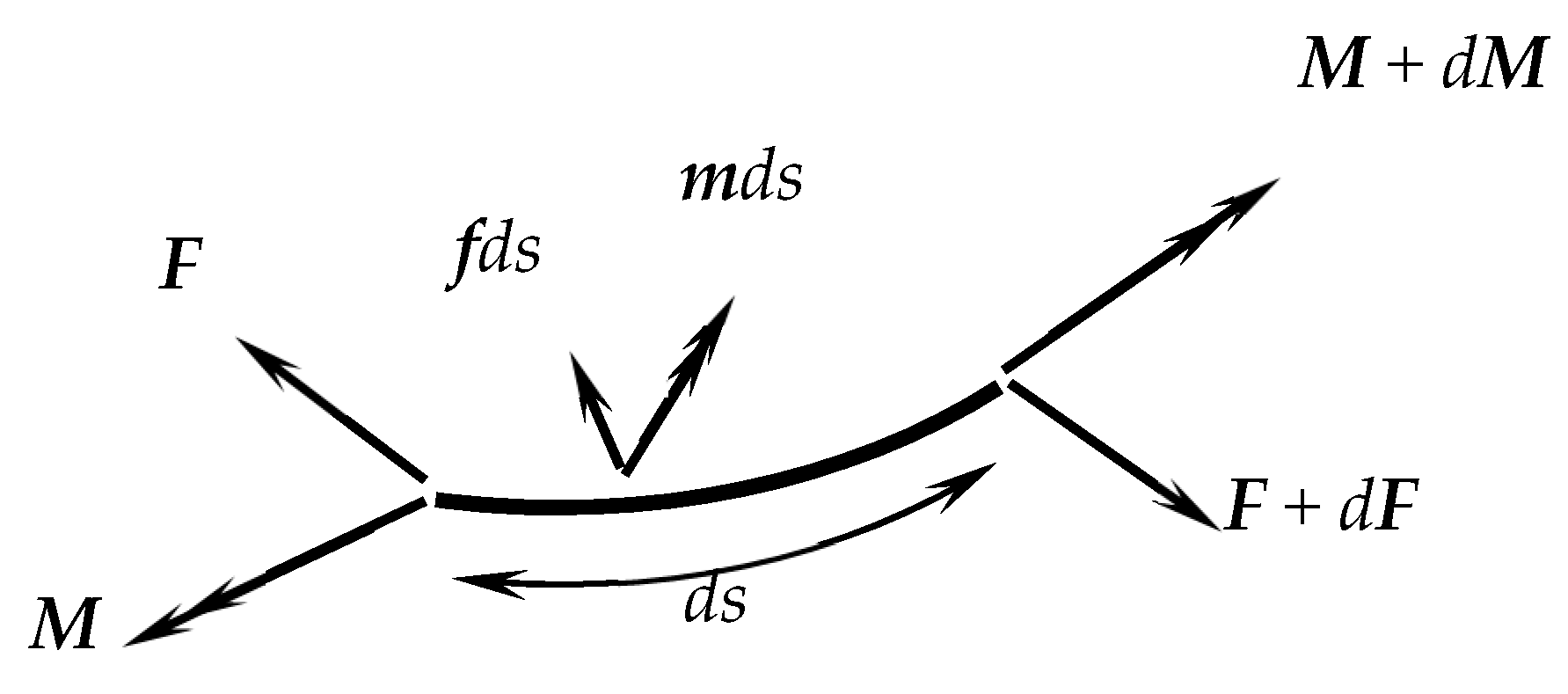
2.3. Equilibrium and Constitutive Equations

As shown in Figure 2, the fulfilment of equilibrium of the beam segment with distributed forces and moments has to satisfy the following conditions:

dF_XYZ/ds + f = 0

(18)

dM_XYZ/ds + (dr/ds) × F_XYZ + m = 0.

(19)

The co-rotational scheme means the equilibrium condition can be constructed directly with respect to the local coordinate system. Hence, Equations (21) and (22) can be given by the following transformation:

dG_XYZ/ds = dG_xyz/ds + ω × G,

(20)

where G_XYZ and G_xyz represent any vector with reference to the global coordinate and local coordinate, respectively:

dF_xyz/ds + ω × F + f = 0

(21)

dM_xyz/ds + ω × M + e_z × F + m = 0.

(22)

In the present study, we established the constitutive equations with the Timoshenko beam hypothesis. Therefore, the constitutive laws between the external forces and deformation can be expressed as follows:

M_x = EI_xx (ω_x − ω_xo + dγ_y/ds)

(23)

M_y = EI_yy (ω_y − ω_yo − dγ_x/ds)

(24)

M_z = GJ (ω_z − ω_zo)

(25)

F_x = k_xGAγ_x

(26)

F_y = k_yGAγ_y

(27)

F_z = EAε

(28)

where E is the Young’s modulus, A is the cross-sectional area, J is the torsional constant, G is the shear modulus, ε is the axial strain of beam axis, γ_x and γ_y are the average shear strain, k_x and k_y are the shear modificatory factors, and I_xx and I_yy are the moments of inertia about the x and y axes, respectively.

2.4. Governing Equations

The above equations have been constructed from the arc length of the beam axis, s, at the deformed configuration. For the convenience of later derivation, the equations can be represented with respect to the arc length of the undeformed beam axis, S, by the relationship of the chord length between the undeformed and deformed configuration as follows:

$$df/ds={(1+F_z/EA)}^{-1}(df/dS).$$

(29)

Substituting Equation (29) into the kinematics and equilibrium equations leads to the governing equations:

$$dX/dS=(1+F_z/EA)\left[\frac{\phi \psi }{{\vartheta }^2}(1-\cos \vartheta )+\frac{\chi }{\vartheta }\sin \vartheta \right]$$

(30)

$$dY/dS=(1+F_z/EA)\left[\frac{\psi \chi }{{\vartheta }^2}(1-\cos \vartheta )-\frac{\phi }{\vartheta }\sin \vartheta \right]$$

(31)

$$dZ/dS=(1+F_z/EA)\left[1-\left[1-{(\frac{\psi }{\vartheta })}^2\right](1-\cos \vartheta )\right]$$

(32)

$$\begin{array}{c}d\phi /dS=\frac{(1+F_z/EA)}{2{\vartheta }^2}[2{\omega }_x{\phi }^2+{\vartheta }^2({\omega }_z\chi -{\omega }_y\psi )\\ +2\phi ({\omega }_y\chi +{\omega }_z\psi )+\vartheta (-{\omega }_y\phi \chi -{\omega }_z\phi \psi +{\omega }_x({\chi }^2+{\psi }^2))\cot \frac{\vartheta }{2}\end{array}$$

(33)

$$\begin{array}{c}d\chi /dS=\frac{(1+F_z/EA)}{2{\vartheta }^2}[2\chi ({\omega }_x\phi +{\omega }_y\chi )+{\omega }_x({\phi }^2+{\chi }^2)\psi +{\omega }_x{\psi }^3\\ -{\omega }_z({\phi }^3-2\chi \psi +\phi ({\chi }^2+{\psi }^2))+\vartheta (-\chi ({\omega }_x\phi +{\omega }_z\psi )+{\omega }_y({\phi }^2+{\psi }^2))\cot \frac{\vartheta }{2}]\end{array}$$

(34)

$$\begin{array}{c}d\psi /dS=\frac{(1+F_z/EA)}{2{\vartheta }^2}[({\omega }_y\phi -{\omega }_x\chi )({\phi }^2+{\chi }^2)+2({\omega }_x\phi +{\omega }_y\chi )\psi \\ +(2{\omega }_z+{\omega }_y\phi -{\omega }_x\chi ){\psi }^2+\vartheta ({\omega }_z({\phi }^2+{\chi }^2)-({\omega }_x\phi +{\omega }_y\chi )\psi )\cot \frac{\vartheta }{2}]\end{array}$$

(35)

$$d{F}_x/dS=(1+F_z/EA)({\omega }_z{F}_y-{\omega }_y{F}_z-f_x)$$

(36)

$$d{F}_y/dS=(1+F_z/EA)({\omega }_x{F}_z-{\omega }_z{F}_x-f_y)$$

(37)

$$d{F}_z/dS=(1+F_z/EA)({\omega }_y{F}_x-{\omega }_x{F}_y-f_z)$$

(38)

$$d{M}_x/dS=(1+F_z/EA)({\omega }_z{M}_y-{\omega }_y{M}_z+F_y-m_x)$$

(39)

$$d{M}_y/dS=(1+F_z/EA)({\omega }_x{M}_z-{\omega }_z{M}_x-F_x-m_y)$$

(40)

$$d{M}_z/dS=(1+F_z/EA)({\omega }_y{M}_x-{\omega }_x{M}_y-m_z)$$

(41)

where

$${\omega }_x=M_x/E{I}_{xx}+{\omega }_x{}_0-(1+F_z/EA)d(F_y/{\kappa }_{y}GA)/dS$$

(42)

$${\omega }_y=M_y/E{I}_{yy}+{\omega }_y{}_0+(1+F_z/EA)d(F_x/{\kappa }_{x}GA)/dS$$

(43)

$${\omega }_z=M_z/GJ+{\omega }_z{}_0$$

(44)

The 12 nonlinear ordinary differential equations, Equations (30)–(41), are derived to solve the spatial beam with naturally curved and twisted beams undergoing large deformations.

3. Differential Reproducing Kernel Approximation Collocation Method (DRK)

3.1. Reproducing Kernel Approximation

Most numerical methods transform a differential equation into the integration form while solving it, such as the Galerkin method [23,27]. However, the DRK approximations adopted in this paper can circumvent the numerical mesh for numerical integration. The DRK collocation method is developed based on the DRK approximation [32,33,34]. The DRK approximation can be derived from the kernel function with a reproducing condition or the moving least square method. Two kinds of derivations represent different characteristics of the DRK approximation. In this section, a brief introduction is given with regard to the moving least square method. Consider a set of N nodal points scattered in a domain Ω and let x* be the reference point. The DRK approximation of a variable u(x) in the neighborhood of the reference point x*, denoted by u^h(x), is

$$u\left(\mathit{x}\right)\approx u^h\left(x\right)={\displaystyle \sum _{i=1}^M{p}_i}\left({\mathit{x}}^{*}-\mathit{x}\right)a_i={\mathit{p}}^T\left({\mathit{x}}^{*}-\mathit{x}\right)\mathit{a}$$

(45)

where ${\mathit{p}}^T=\left\{p_1(\mathit{x}),p_2(\mathit{x}),\dots ,p_M(\mathit{x})\right\}$ is a linear independent basis; $a^T=\left\{a_1,a_2,\dots ,a_M\right\}$ is a vector of undetermined coefficients. Hence, the error in the weighted least-squares of N nodes at neighborhood with respect to the reference point x* can be expressed as follows:

$$\begin{array}{ll}J& ={\displaystyle \sum _{i=1}^{Ne}{w}_a(x^{*}-x_j){[p^T(x^{*}-x_j)a-u(x_j)]}^2}\\ & =(a^{T}P(x^{*})-u^T)W(x^{*})(P^T(x^{*})a-u)\end{array}$$

(46)

where $w_a({\mathit{x}}^{*}-\mathit{x})$ is the local weight function and Ne is the number of neighboring nodes of x*. The index a is the radius of support and u(x_j) is the approximation of u(x) at node x_j. By minimizing the error of the weighted least-square, the approximation u^h(x) can be obtained as follows:

$$u^h(x)=p^T(x^{*}-x)M^{-1}(x^{*})B(x^{*})u=N^T(x;x^{*})u,$$

(47)

where $M(x^{*})=P(x^{*})W(x^{*})P^T(x^{*})$, $B(x^{*})=P(x^{*})W(x^{*})$, $u^T=\left\{u(x_1),u(x_2),\dots u(x_N)\right\}$ and $N^T(x;x^{*})$ is the shape function that can be defined as follows:

$$N^T(x;x^{*})=p^T(x^{*}-x){\mathit{M}}^{-1}(x^{*})B(x^{*})$$

(48)

The approximation u^h(x) in Equation (47) is a local approximation in the neighborhood with respect to the refence point x*. However, the global approximation can be fulfilled by the moving least-square method by imposing x = x* such that point x* will move with the point that has to be computed. In this way, the global approximation can be expressed as follows:

$$u^h(x)=p^T(0)M^{-1}(x)B(x)u=N^T(x)u$$

(49)

where $N^T(x)=p^T(0)M^{{}^{-1}}(x)B(x)$.

3.2. Differential Reproducing Kernel Approximation

Different from conventional RK approximants, the derivatives of the shape function in DRK are computed by differentiating toward the reproducing condition instead of directly with a shape function. Hence, no special treatment is needed in DRK while computing a different order derivative of the shape function. The derivative of the reproducing kernel function can be obtained by differentiating Equation (47) directly:

$$\frac{{\partial }^k{N}^T\left(x;x^{*}\right)}{\partial x^k}=\frac{{\partial }^k{p}^T(x^{*}-x)}{\partial x^k}{M}^{-1}(x^{*})\mathrm{B}(x^{*})$$

(50)

By moving the least squares method and imposing x = x*, the derivatives of the global approximation can be obtained as follows:

$$\frac{{\partial }^k{N}^T\left(x\right)}{\partial x^k}=\frac{{\partial }^k{p}^T(x^{*}-x)}{\partial x^k}|{}_{x=x^{*}}{M}^{-1}(x)\mathrm{B}(x)$$

(51)

Thus, the procedures for computing the different order derivative in DRK are the same. In addition, by imposing the point collocation method with the moving least squares method, a boundary valued problem can be expressed as in the following equations:

$$L_{\mathsf{\Omega }}\{p^T(x^{*}-x)\}|{}_{x=x^{*}}{M}^{-1}(x_j)B(x_j)u=f(x_j)$$

(52)

$$L_{\partial \mathsf{\Omega }}\{p^T(x^{*}-x)\}|{}_{x=x^{*}}{M}^{-1}(x_j)B(x_j)u=g(x_j)$$

(53)

where $\mathsf{\Omega }$ and $\partial \mathsf{\Omega }$ are the domain and boundary of the problem; $L_{\mathsf{\Omega }}$ and $L_{\partial \mathsf{\Omega }}$ are linear differential operators. If the number of nodes in the domain is N_p, the number of nodes on the boundary is N_b. Equations (52) and (53) lead to

$$G_{(Np+Nb)\times Np}{u}_{Np\times 1}=f_{(Np+Nb)\times 1}$$

(54)

The variables in the above equation are unknown, so the least squares method is adopted to find the optimum solutions.

Similar to most meshfree methods, the influence of the nodal values of the neighboring nodes is estimated by the weight function. Therefore, domain ${\mathsf{\Omega }}_I$ should contain the nodal point $x^{*}$ itself and also make the shape function to be zero outside. In the following analysis, the cubic spline is adopted to be the weight function as follows:

$$w\left(d\right)=\{\begin{array}{c}\frac{2}{3}-4d^2+4d^3\\ \frac{4}{3}-4d+4d^2-\frac{4}{3}{d}^3\\ 0\end{array}\begin{array}{c}ford\le \frac{1}{2}\\ for\frac{1}{2}<d\le 1\\ ford>1\end{array},$$

(55)

where the normal distance $d=|x_j-x^{*}|/a$ and a is the radius of support.

However, the radius of support also has to be small enough to exhibit the local character and cannot be too small to yield an ill-conditioned problem at the same time. Hence, it is necessary to determine the optimum range of radius of support. The present scheme is capable of tuning with the density of nodes automatically such that the radius of support can exhibit the local character and not lead to an ill-conditioned problem. For a point at $x^{*}$, the number of neighboring nodes, Ne, is determined by the order of basis functions. Then we can sort the neighboring nodes by the distance to the point $x^{*}$. The distance of the Ne-th neighboring node is adopted as the radius of support. In this way, the radius of support can be tuned automatically with the density of nodes instead of being fixed.

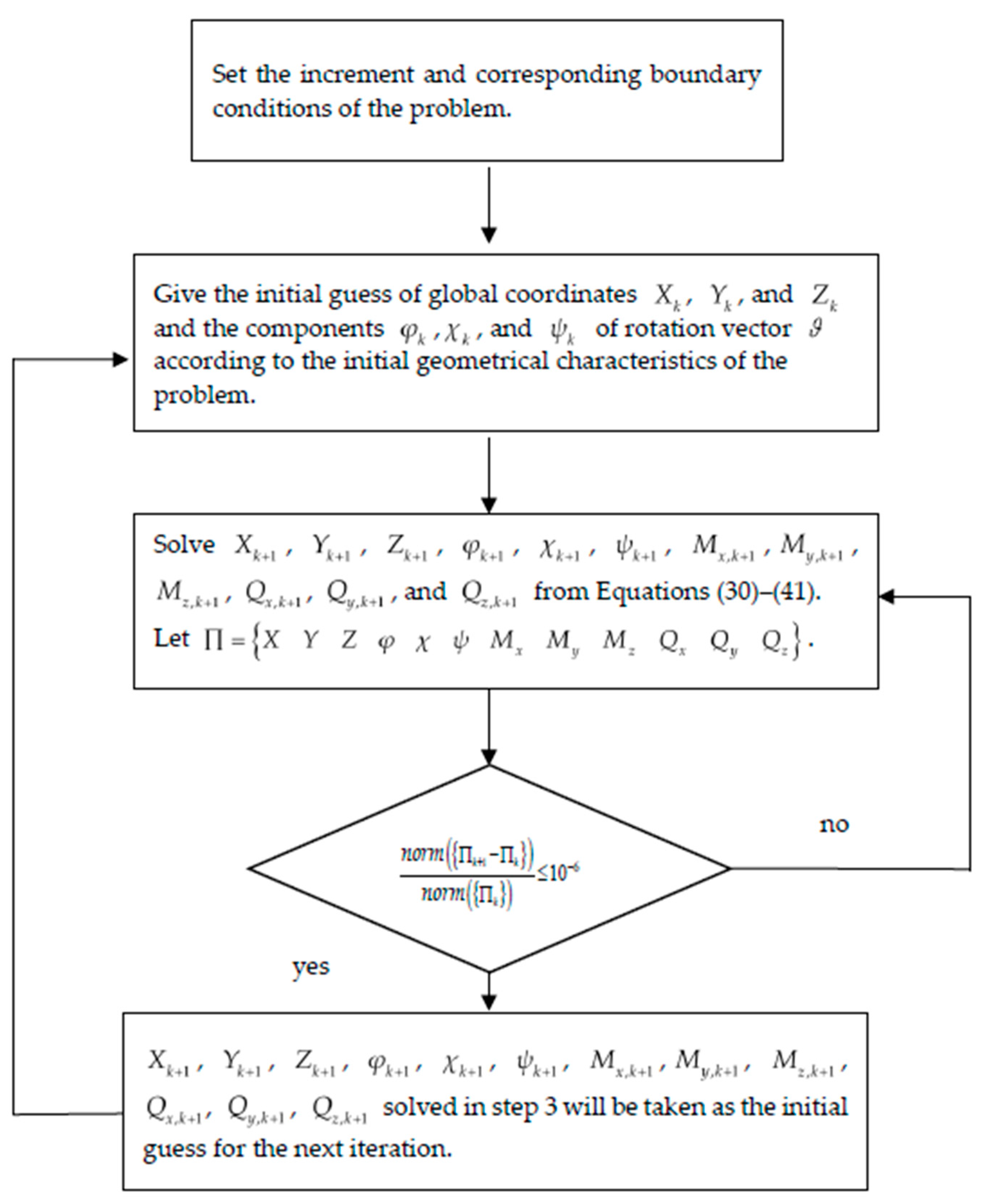
3.3. Strategy for Incremental–Iterative Procedure

An incremental–iterative method combining the DRK approximations with the Newton–Raphson method was adopted to solve the 12 coupled, nonlinear ordinary differential equations, Equations (30)–(41). In the present incremental–iterative procedure, force or displacement will be adopted as the prescribed increment. Whichever kind of increment is adopted, the solution from the preceding iteration will be taken as the new initial guess for the next one. Let $X_k$, $Y_k$, $Z_k$, ${\phi }_k$, ${\chi }_k$, ${\psi }_k$, $M_{x,k}$, $M_{y,k}$, $M_{z,k}$, $Q_{x,k}$, $Q_{y,k}$, and $Q_{z,k}$ denote the solutions of the Kth incremental step. The incremental–iterative steps adopted in the present scheme are as shown in Figure 3.

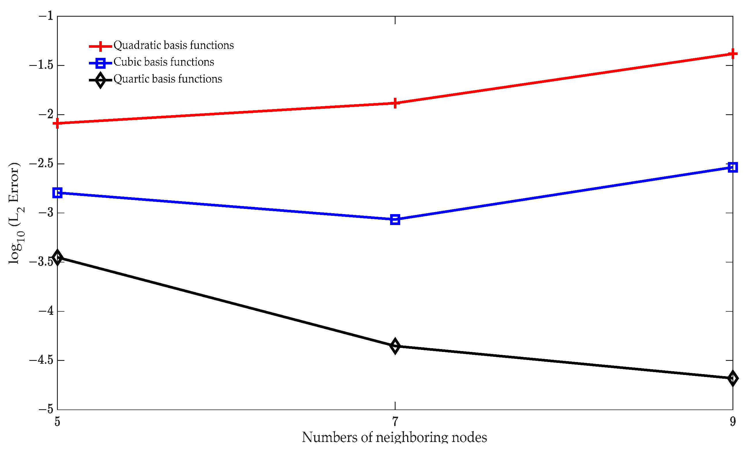
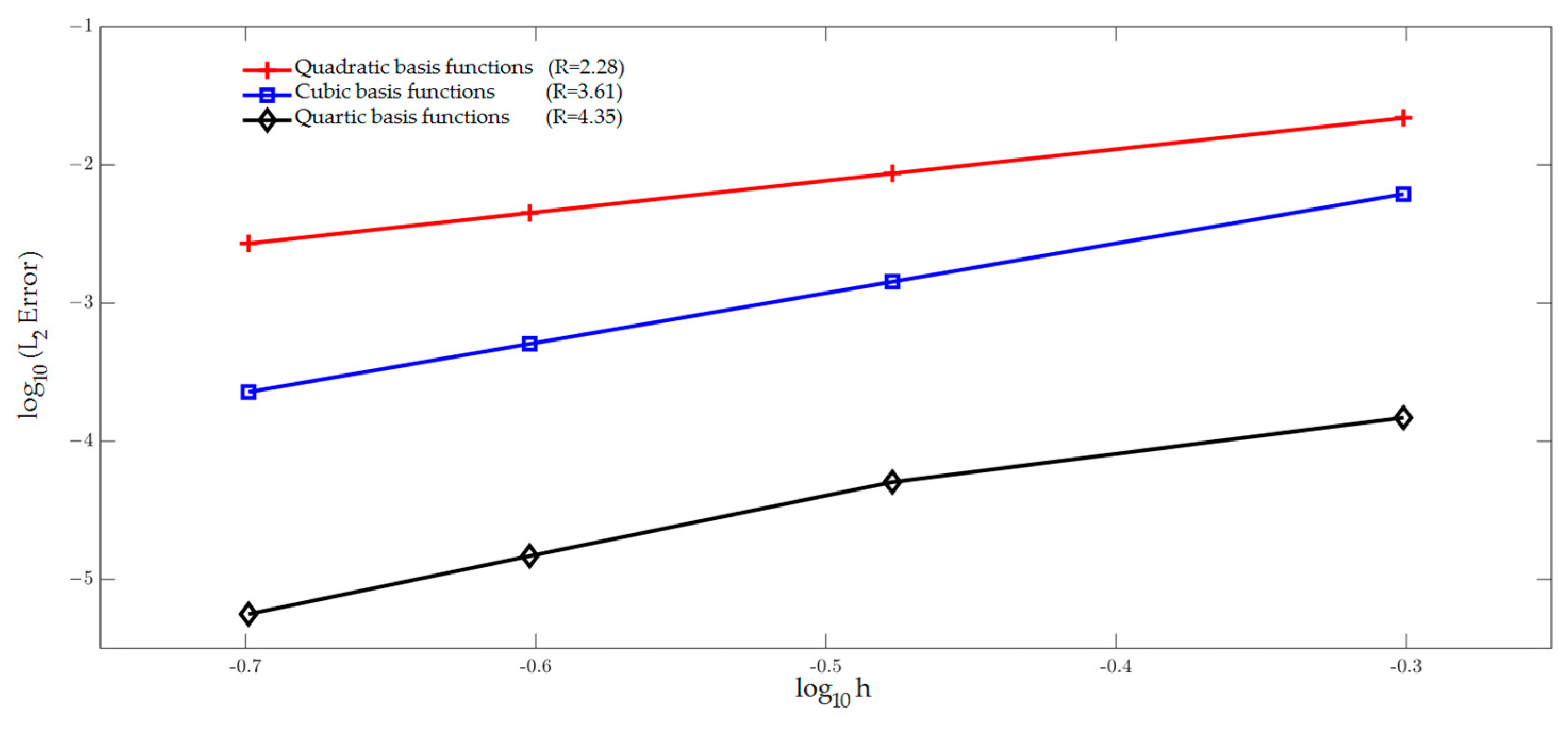
4. Numerical Examples

Five numerical examples, including large deformation, postbuckling of two-dimensional beam structures, stability, and lateral buckling problems of three-dimensional beam structures, are presented to show the effectiveness and performance of the proposed three-dimensional co-rotational beam formulation.

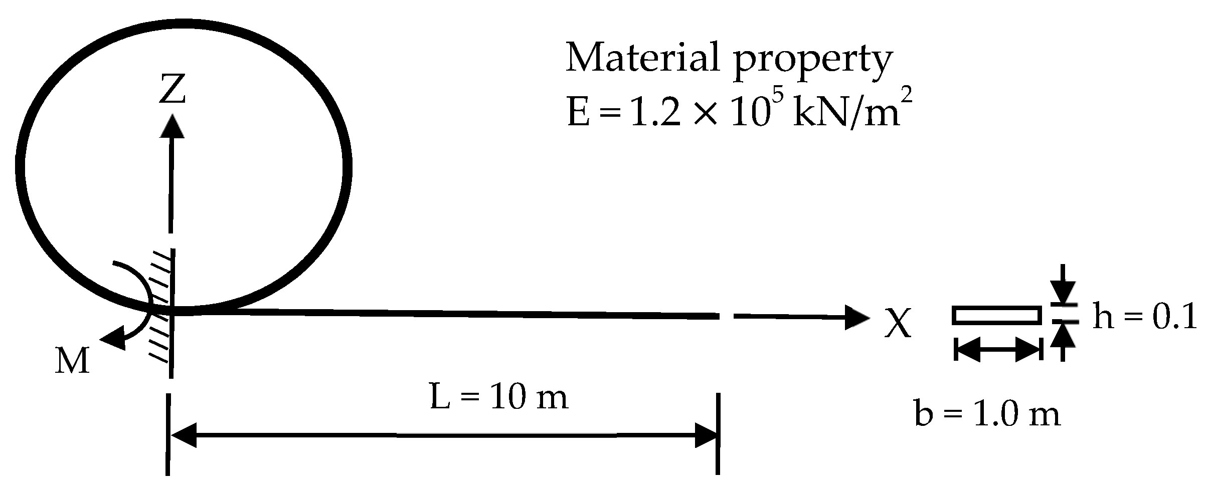
4.1. Cantilever Curved Beam Subjected to End Moment

Figure 4 represents the geometrically nonlinear analysis of a cantilever curved beam with an initial circle shape such that the fixed and free ends can be reduplicated. The geometry and material properties of the curved beam are: L = 10.0 m, b = 1.0 m, h = 0.1 m, and E = 1.2 × 10⁵ kN/m². The basic equation of the fixed global coordinates and end moment can be written as follows:

$$Z^2+X^2={\left(\frac{EI}{M}\right)}^2$$

(56)

Hence, a curved beam with an initial circular shape will bend into a straight beam when the end moment, $M=\left(\frac{2\pi EI}{L}\right)$, is applied. If the end moment reaches $M=\left(\frac{4\pi EI}{L}\right)$, the beam will bend into a circle in the opposite direction.

To find the optimal number of neighboring nodes and order of basis function, the L2 error for a combination of neighboring nodes 3, 5, and 7 with respect to the basis functions of quadratic, cubic, and quartic was plotted in Figure 5. It shows that the optimal relationship between the number of the neighboring nodes and basis functions can be given as follows:

Ne = (2m − 1),

(57)

where Ne is the number of the neighboring nodes and m is the number of basis functions. The computational time of the above combinations shown in Figure 5 was less than 10 s. Additionally, the above optimal combination of neighboring nodes with order of basis function was adopted to plot Figure 6, which shows the convergence corresponding to the number of nodal points of 21, 31, 41, and 51 with quadratic, cubic, and quartic basis functions, respectively. It should be noted that h, shown in Figure 6, means the spacing of nodal points. The results show that the DRK approximations with a higher degree basis and more nodal points can effectively improve the solution accuracy. Moreover, the higher degree basis functions will achieve better solution accuracy even if the same number of nodal points is adopted. A combination of quadratic basis functions and five neighboring nodes was adopted in the following examples.

The moment–displacement curves of the curved cantilever beam are plotted in Figure 7, solved by 31 nodal points with 10 loading increments. The number of iterations of each increment is less than three. As can be seen, the present theory can provide accurate solutions.

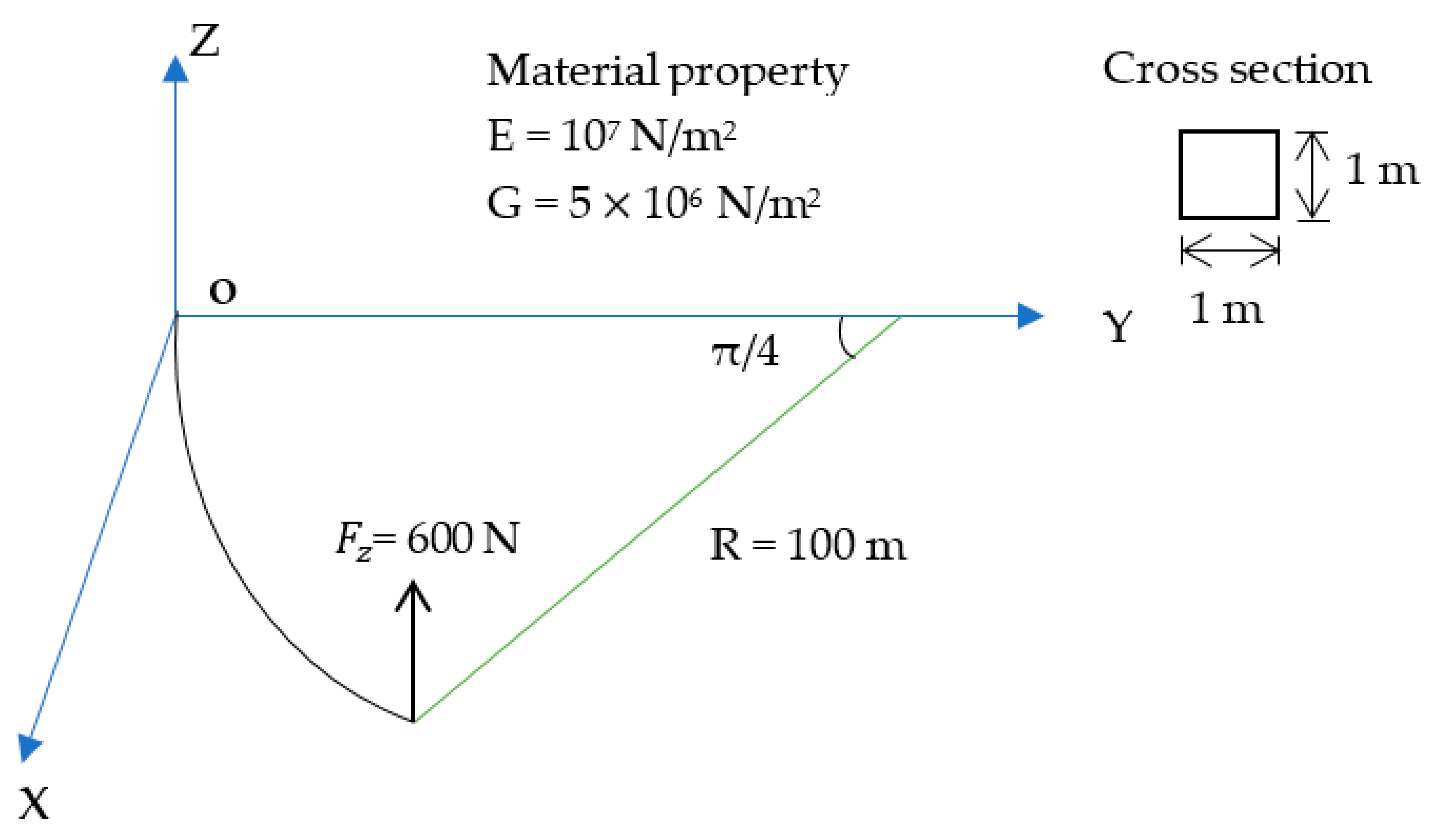
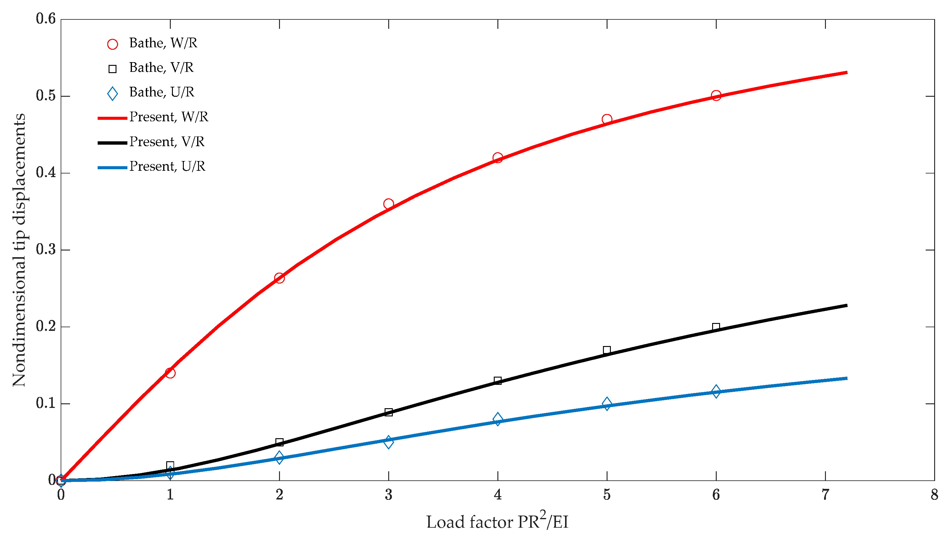
4.2. A cantilever Beam Initially Curved to π/4 Subjected to a Concentrated Tip Load

As shown in Figure 8, a cantilever beam initially curved to an arch of radius 100 m with 45-degree bending was subjected to a concentrated end load. This example was originally proposed by Bathe [1] and has also been adopted by a number of other researchers [2,3,12,13,21]. The beam has a unit square cross section and lies in the X–Y plane with initial tip position 70.71 m, 29.29 m, 0 m of the fixed X–Y–Z global coordinates. The material was linear and elastic, with the following properties: Elastic modulus, E = 10⁷ N/m², and Shear modulus, G = 5 × 10⁶ N/m². In the above reference, the beam was modeled by straight and curved beam elements with the nodes on the centroidal axis of the beam. In the present study, DRK was fulfilled by nodal points to simulate a beam undergoing large deformation.

Figure 9, solved by 31 nodal points with 10 loading increments, shows the evolution of tip displacement as a function of the applied load modulus. The number of iterations is fewer than five within each increment.

Table 1. Free-end position of the cantilever 45-degree under out-of-plane force.

Model	Nelm	Nnode	X	Y	Z
Present		31	47.89	15.96	53.10
Bathe and Bolourchi [1]	-		47.20	15.90	53.4
Simo and Vu-Quoc [2]	8 (linear, straight)		47.23	15.79	53.37
Cardona and Geradin [3]	8 (linear, straight)		47.04	15.96	53.50
Zupan et al. [13]	8 (linear, curved)		46.89	15.61	53.60
Magisano et al. [21]	4 (CR-Incremental)		-	-	53.47

shows the free end position of the initial curved cantilever beam under out-of-plane force. A comparison of the free end position from these references is also given in Table 1. The results show that the present theory can provide accurate solutions.

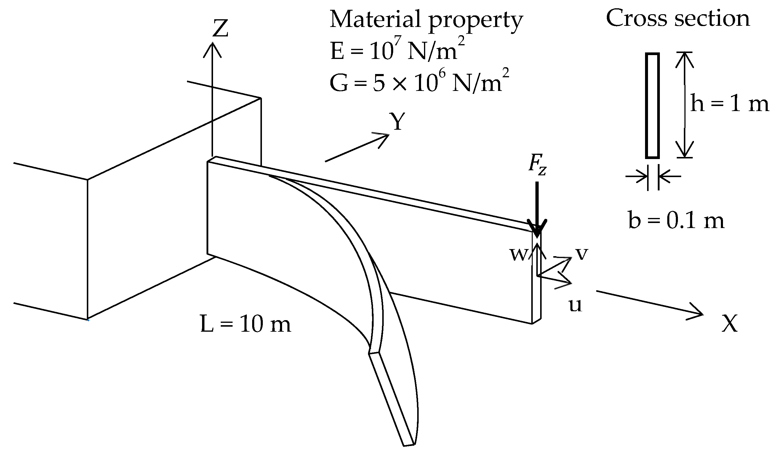
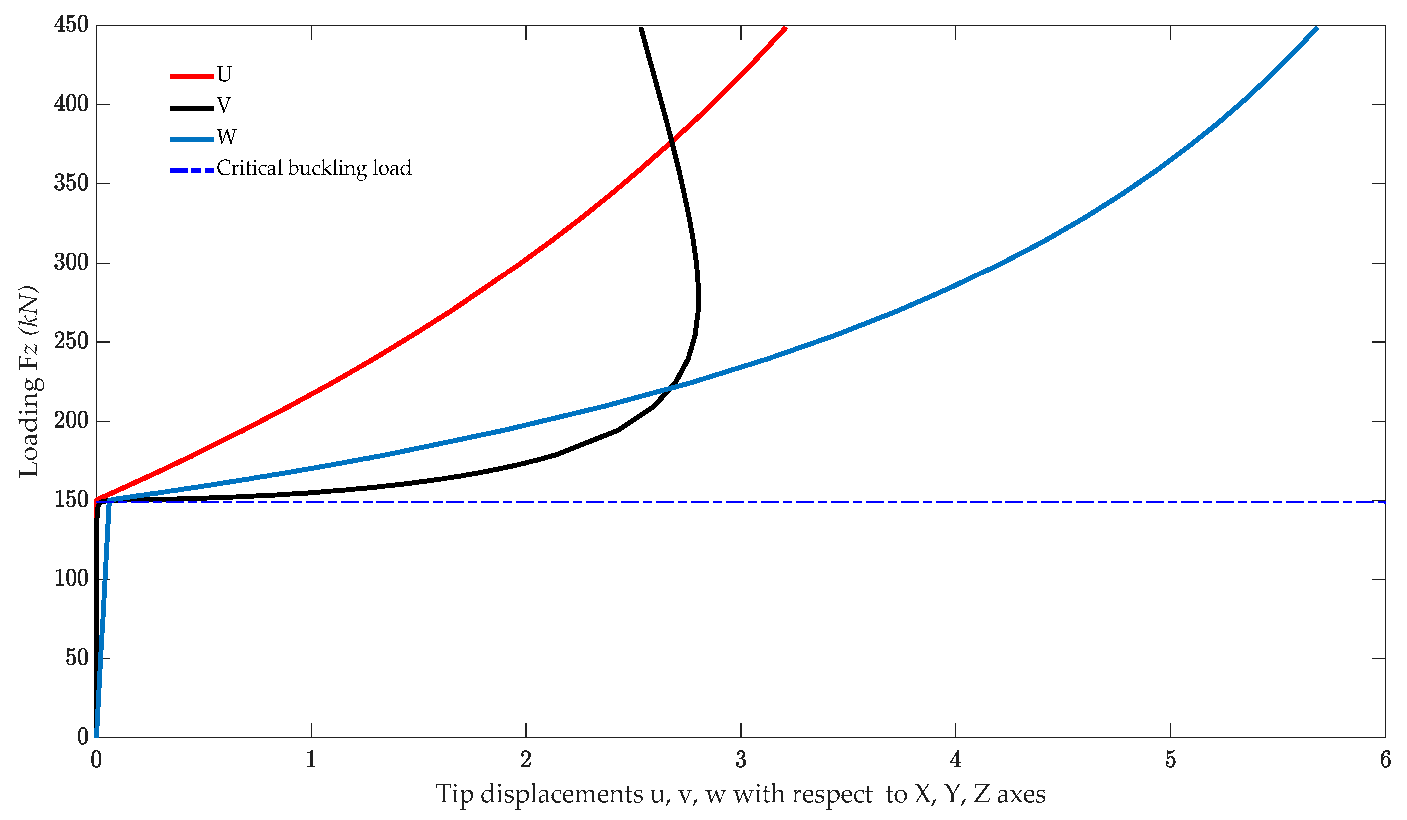
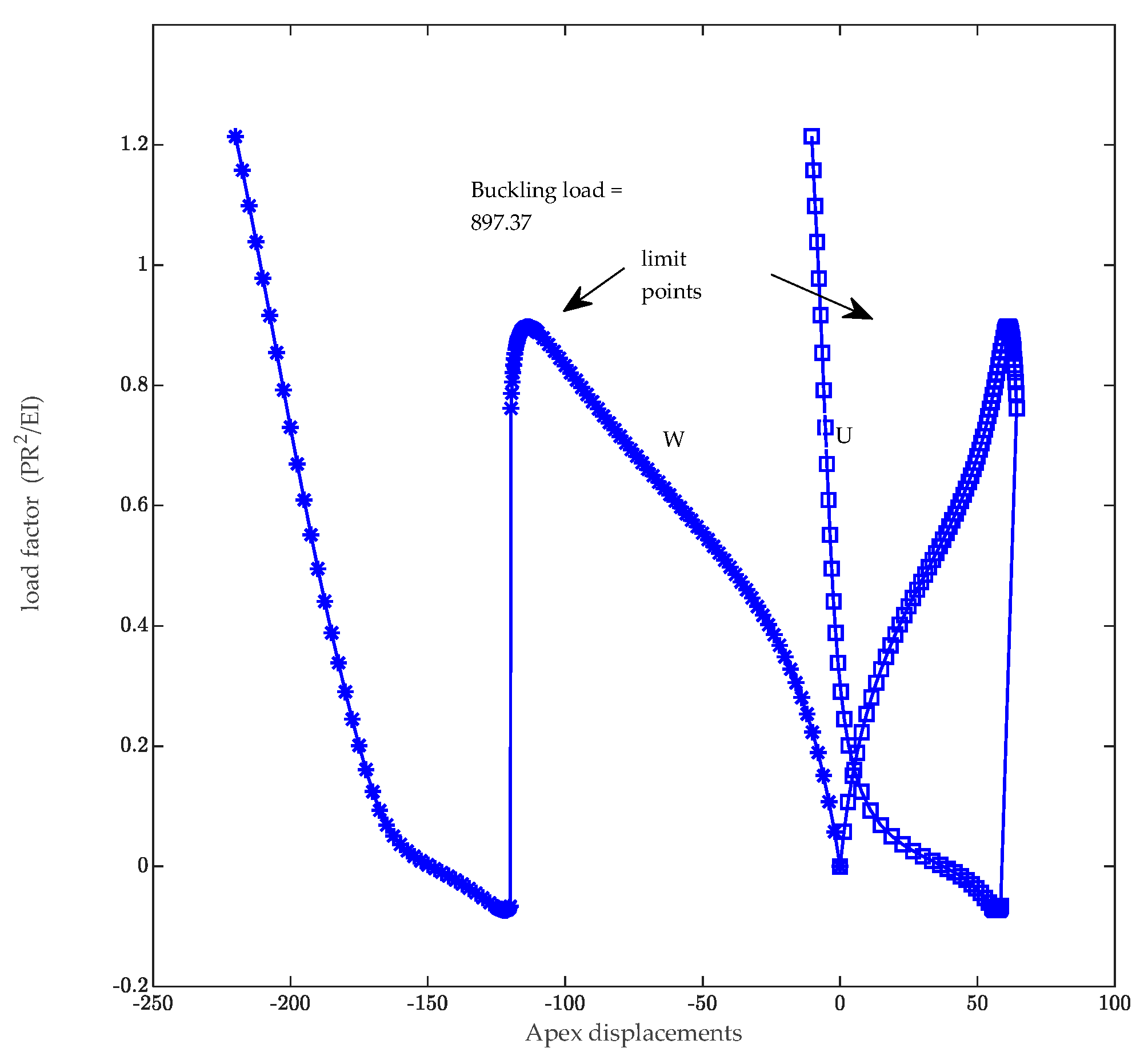
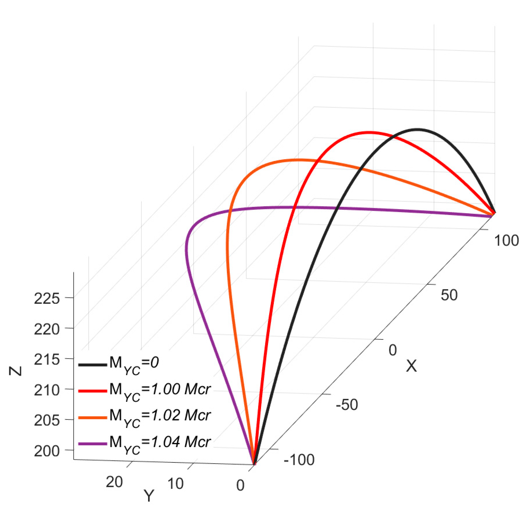
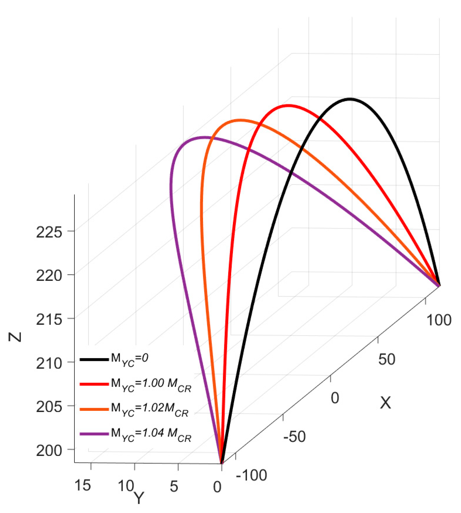
4.3. Lateral Buckling of a Cantilever Beam

This example presents the lateral buckling of a cantilever beam with a narrow rectangular cross section. As shown in Figure 10, a transverse force, Fz, is loaded on the direction of the strong axis of the cross section. The geometry and material properties of the cantilever beam are: E = 10⁷ kN/m², G = 5 × 10⁶ kN/m², b = 0.1 m, h = 1.0 m, and L = 10.0 m. The theoretical buckling load is given by Timoshenko [36] as follows:

$$P_{cr}=\frac{4.013599344\sqrt{{EI}_{x}GJ}}{L^2}$$

(58)

where EI_x is the flexural rigidity of the weak axis of the cross section, a is the torsional rigidity, and L is the length of the beam. The deformation processes of the cantilever beam with a downward concentrated load up to instability are shown in Figure 11. Figure 12 shows the load deflection curves obtained by 31 nodal points, with 62 loading increments up to three times the buckling load. The number of iterations is fewer than five within each increment. The buckling load, Pcr = 149.557 kN, obtained from Timoshenko [36], was indicated. It can be seen that the present numerical solution agrees well with the analytical solution.

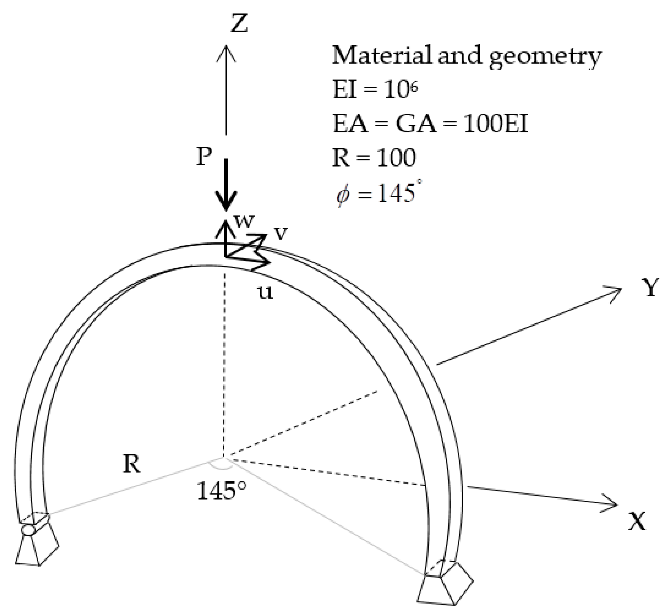
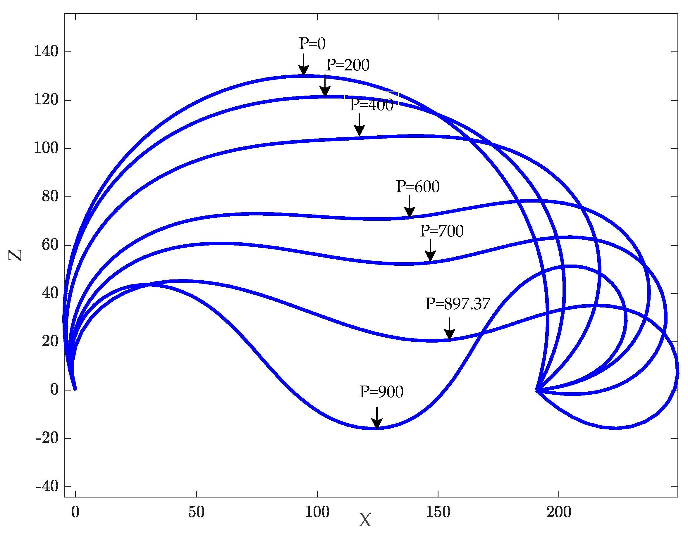
4.4. Postbuckling of a Clamped–Hinged Circular Arch

This famous example presents the geometrically nonlinear analysis of the pre- and postbuckling deformation of the circular arch, clamped at one end and hinged at the other end, with a concentrated load applied at the apex as shown in Figure 13. The material and geometric data for the arch are R = 100, EI = 10⁶, EA = GA = 100EI, $f={145}^{°}$.

Different numbers of nodal points were adopted to evaluate the buckling load, and 72 nodal points were capable of acquiring good results. The deformation processes of the circular arch subject to a concentrated load up to instability are plotted in Figure 14. An analytical solution by DaDeppo and Schmidt is also available in [37]. Figure 15 shows that the load factor–deflection curves of the pre- and postbuckling analysis were solved by 72 nodal points and 136 displacement increments. The number of iterations is fewer than ten within each increment. Moreover, a comparison of numerical solutions of the buckling load with FEM by Simo [2], Ibrahimbegovic [7], and Kapania [12] is given in

Table 2. Buckling load of clamped-hinged circular arch.

Model	Nelm	Nnode	Limit Buckling Load
Present		72	897.37
Simo [1]	40 (2-noded, straight)		905.28
Ibrahimbegovic [5]	20 (3-noded, curved)		897.30
Kapania [11]	6 (4-noded, curved)		897.27
Zupan [13]	80 (3-noded, curved)		897.87
Classical solution			897.00

.

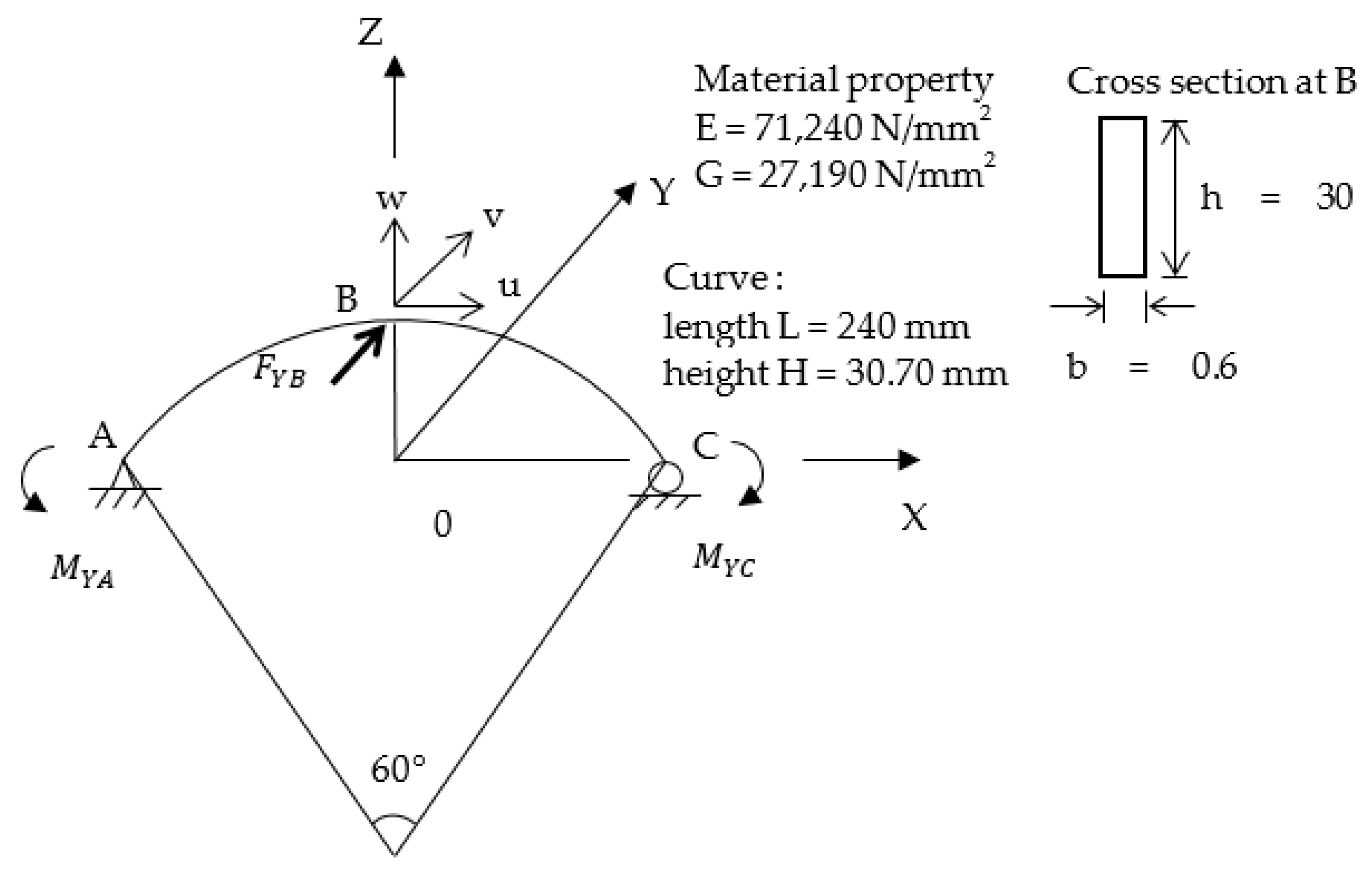
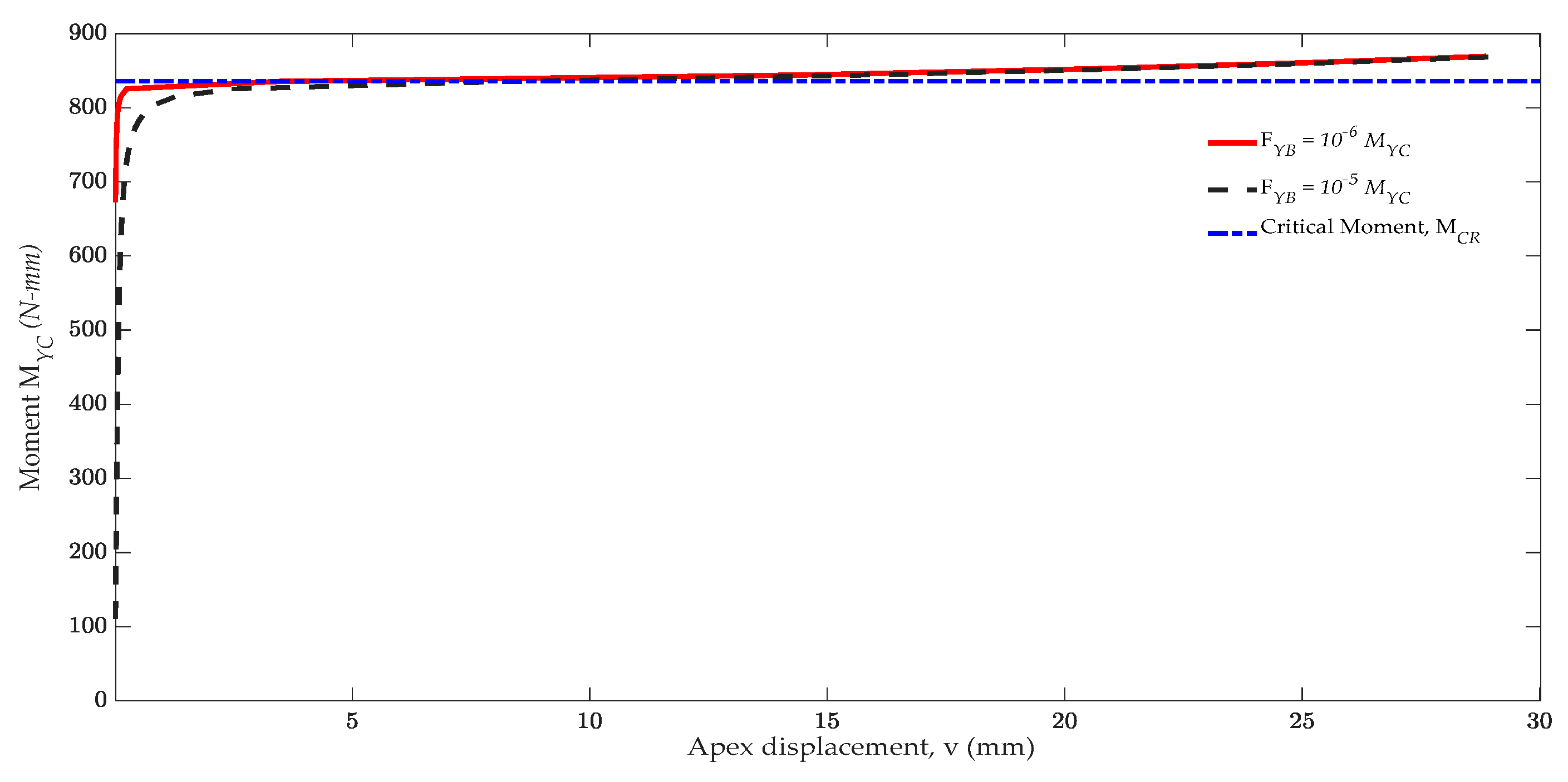
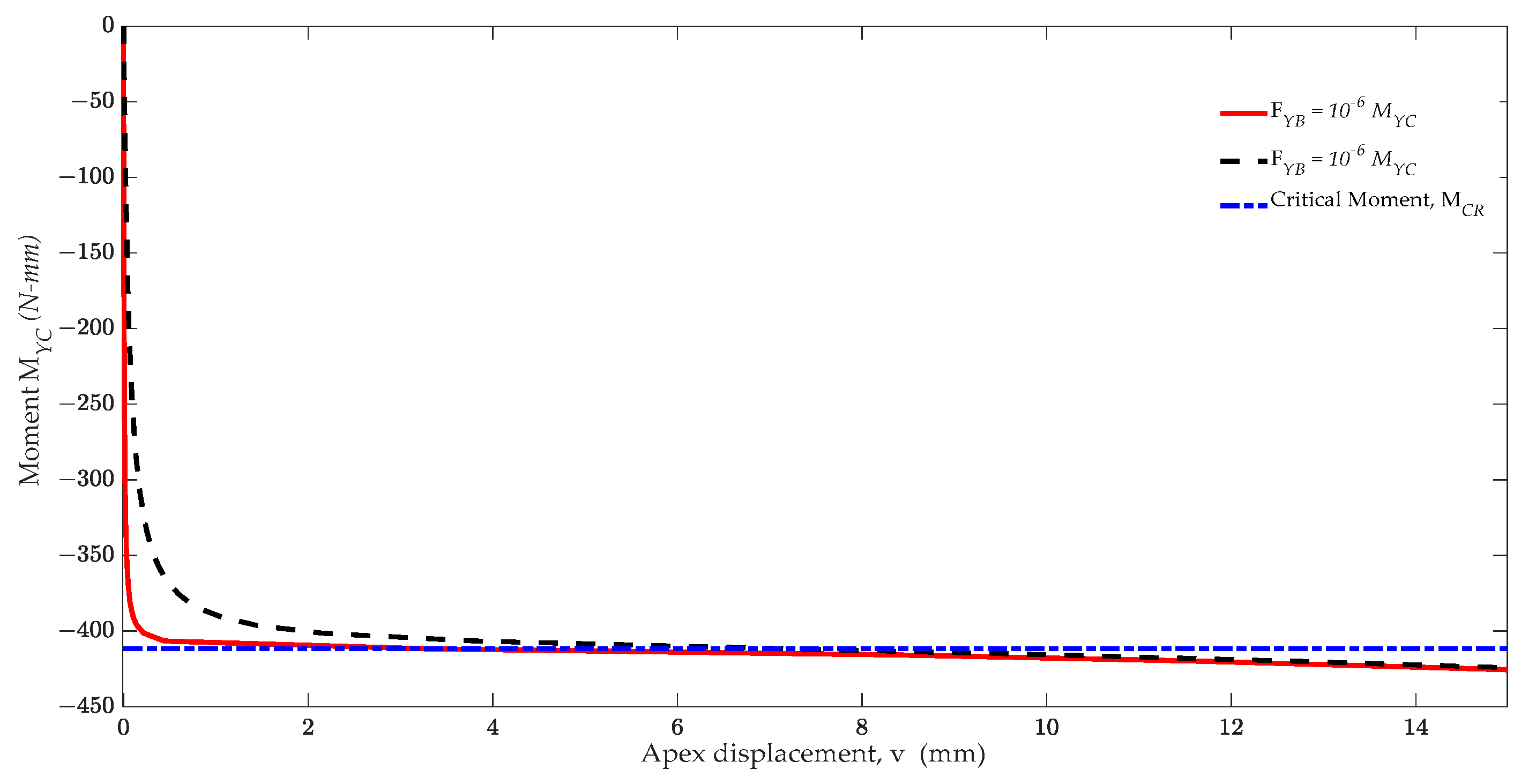
4.5. Lateral Buckling of a Curve Beam

This example presents the performance of the three-dimensional nonlinear analysis of the lateral buckling of a curve beam. As shown in Figure 16, there is a simply supported curve beam with a subtended angle of $60°$. Note that the rotation with respect to the principal axes of inertia of the cross section is allowable, but it is unable to rotate about the normal direction of the cross section. The geometric and material properties of the curved beam are: curve length L = 240 mm, b = 0.6 mm, h = 30 mm, E = 71,240 N/mm², and G = 27,190 N/mm².

A comparison of the effect of imperfect loading is given by several imperfect loadings, F_YB = $\alpha$M_YA, applied at central point B. The coefficients of imperfection loads, $\alpha$, adopted to trigger the lateral deformation, are 10⁻⁵ and 10⁻⁶, respectively. Figure 17 and Figure 18 show the moment–displacement curves associated with different imperfection loads, F_YB, under positive and negative moments, in which 82 nodal points and 36 loading increments were adopted. The maximum number of iterations was seven during the iteration computation. The critical moments, Mcr = 835.82 N-mm and −411.70 N-mm, obtained from the curve beam theory of Yang [38], are also indicated. Moreover, the postbuckling deformation processes of the curved beam from buckling moment, Mcr, to 1.04 Mcr are also shown in Figure 19 and Figure 20.

5. Conclusions

A three-dimensional co-rotational beam formulation for the geometrically nonlinear analysis of a spatial beam was constructed in the context of a co-rotational formulation and Timoshenko beam hypothesis. In this paper, the Rodrigues formula was adopted to represent the finite rotation in a co-rotational scheme; this also circumvents the famous Gimbal lock problem that may occur with rotation in terms of the Euler angle. The numerical implementation of the DRK approximation collocation method, combined with the Newton–Raphson method, directly solved the strong forms of the geometrically nonlinear problems—different from FEM, which solves the weak form by means of the variation method. The present scheme means that the stress field can be solved directly from the governing equations instead of recovering through the differentiation procedure toward the kinematic field. That is, the primary interpolated variables will not be the dominant factor. The scheme presented is also capable of effectively solving geometrically nonlinear analyses such as large deformation, snap-through, postbuckling, and lateral buckling problems. Numerical examples are given to demonstrate the validity and effectiveness.

References

1. Bathe, K.; Bolourchi, S. Large displacement analysis of three-dimensional beam structures. Int. J. Numer. Meth. Eng. 1979, 14, 961–986. [Google Scholar] [CrossRef]
2. Simo, J.C.; Vu-Quoc, L. A three-dimensional finite-strain rod model. Part II: Computational aspects. Comput. Methods Appl. Mech. Eng. 1986, 58, 79–116. [Google Scholar] [CrossRef]
3. Cardona, A.; Geradin, M. A beam finite element non-linear theory with finite rotations. Int. J. Numer. Meth. Eng. 1988, 26, 2403–2438. [Google Scholar] [CrossRef]
4. Crisfield, M.A. A consistent co-rotational formulation for non-linear, three-dimensional, beam elements. Comput. Methods Appl. Mech. Eng. 1990, 81, 131–150. [Google Scholar] [CrossRef]
5. Jelenic, G.; Saje, M. A kinematically exact space finite strain beam model-finite element formulation by generalized virtual work principle. Comput. Methods Appl. Mech. Eng. 1995, 120, 131–161. [Google Scholar] [CrossRef]
6. Ibrahimbegovic, A. On finite element implementation of geometrically nonlinear reissner’s beam theory: Three-dimensional curved beam elements. Comput. Methods Appl. Mech. Eng. 1995, 122, 11–26. [Google Scholar] [CrossRef]
7. Ibrahimbegovic, A.; Shakourzadeh, H.; Batoz, J.L.; Mikdad, M.A.; Guo, Y.Q. On the role of geometrically exact and second-order theories in buckling and post-buckling analysis of three-dimensional beam structures. Comput. Struct. 1996, 61, 1101–1114. [Google Scholar] [CrossRef]
8. Hsiao, K.M.; Yang, R.T.; Lin, W.Y. A consistent finite element formulation for linear buckling analysis of spatial beams. Comput. Methods Appl. Mech. Eng. 1998, 156, 259–276. [Google Scholar] [CrossRef]
9. Jelenic, G.; Crisfield, M.A. Geometrically Exact 3D Beam Theory: Implementation of a strain-invariant finite element for statics and dynamics beams. Comput. Methods Appl. Mech. Eng. 1999, 171, 141–171. [Google Scholar] [CrossRef]
10. Hsiao, K.M.; Lin, W.Y. A co-rotational finite element formulation for buckling and postbuckling analyses of spatial beams. Comput. Methods Appl. Mech. Eng. 2000, 188, 567–594. [Google Scholar] [CrossRef]
11. Yang, Y.B.; Kuo, S.R.; Wu, Y.S. Incrementally small-deformation theory for nonlinear analysis of structural frames. Eng. Struct. 2002, 24, 783–798. [Google Scholar] [CrossRef]
12. Kapania, R.K.; Li, J. A formulation and implementation of geometrically exact curved beam elements incorporating finite strains and finite rotations. Comput. Mech. 2003, 30, 444–459. [Google Scholar] [CrossRef]
13. Zupan, D.; Saje, M. Finite-element formulation of geometrically exact three-dimensional beam theories based on interpolation of strain measures. Comput. Methods Appl. Mech. Eng. 2003, 192, 5209–5248. [Google Scholar] [CrossRef] [Green Version]
14. Zupan, D.; Saje, M. The three-dimensional beam theory: Finite element formulation based on curvature. Comput. Struct. 2003, 81, 1875–1888. [Google Scholar] [CrossRef]
15. Makinen, J. Total lagrangian reissner’s geometrically exact beam element without singularities. Int. J. Numer. Meth. Eng. 2007, 70, 1009–1048. [Google Scholar] [CrossRef]
16. Cannarozzi, M.; Molari, L. Stress-based formulation for non-linear analysis of planar elastic curved beams. Int. J. Nonlin. Mech. 2013, 55, 35–47. [Google Scholar] [CrossRef]
17. Ye, J.; Xu, L. Member discrete element method for static and dynamic responses analysis of steel frames with semi-rigid joints. Appl. Sci. 2017, 7, 714. [Google Scholar] [CrossRef] [Green Version]
18. Silva, R.; Lavall, A.; Costa, R.; Viana, H. Formulation for second-order inelastic analysis of steel frames including shear deformation effect. J. Constr. Steel. Res. 2018, 151, 216–227. [Google Scholar] [CrossRef]
19. Piotrowski, R.; Szychowski, A. Lateral torsional buckling of steel beams elastically restrained at the support nodes. Appl. Sci. 2019, 9, 1944. [Google Scholar] [CrossRef] [Green Version]
20. Reissner, E. On finite deformation of space-curved beams. J. Appl. Math. Phys. 1981, 32, 734–744. [Google Scholar] [CrossRef]
21. Magisano, D.; Leonetti, L.; Madeo, A.; Garcea, G. A large rotation finite element analysis of 3D beams by incremental rotation vector and exact strain measure with all the desirable features. Comput. Methods Appl. Mech. Eng. 2020, 361, 112811. [Google Scholar] [CrossRef]
22. Magisano, D.; Leonetti, L.; Garcea, G. How to improve efficiency and robustness of the Newton method in geometrically non-linear structural problem discretized via displacement-based finite elements. Comput. Methods Appl. Mech. Eng. 2017, 313, 986–1005. [Google Scholar] [CrossRef]
23. Belytschko, T.; Lu, Y.Y.; Gu, L. Element-free Galerkin methods. Int. J. Numer. Meth. Eng. 1994, 37, 229–256. [Google Scholar] [CrossRef]
24. Liu, W.K.; Jun, S.; Zhang, Y.F. Reproducing kernel particle methods. Int. J. Numer. Meth. Fluids 1995, 20, 1081–1106. [Google Scholar] [CrossRef]
25. Li, S.; Liu, W.K. Reproducing kernel hierarchical partition of unity. Part I: Formulation and Theory. Int. J. Numer. Meth. Eng. 1999, 45, 251–288. [Google Scholar] [CrossRef]
26. Atluri, S.N.; Zhu, T. New concepts in meshless methods. Int. J. Numer. Meth. Eng. 2000, 47, 537–556. [Google Scholar] [CrossRef]
27. Atluri, S.N.; Shen, S. The Meshless Local Petrov-Galerkin Method; Tech. Science Press: Los Angeles, CA, USA, 2002. [Google Scholar]
28. Aluru, N.R. A point collocation method based on reproducing kernel approximations. Int. J. Numer. Meth. Eng. 2000, 47, 1083–1121. [Google Scholar] [CrossRef]
29. Onate, E.; Perazzo, F.; Miquel, J. A finite point method for elasticity problems. Comput. Struct. 2001, 79, 2151–2163. [Google Scholar] [CrossRef]
30. Yang, J.P.; Chen, J.Y. Strong-form formulated generalized displacement control method for large deformation analysis. Int. J. Appl. Mech. 2017, 9, 1750101. [Google Scholar] [CrossRef]
31. Wang, D.; Wang, J.; Wu, J. Superconvergent gradient smoothing meshfree collocation method. Comput. Methods Appl. Mech. Eng. 2018, 340, 728–766. [Google Scholar] [CrossRef]
32. Wang, Y.M.; Chen, S.M.; Wu, C.P. A meshless collocation method based on the differential reproducing kernel interpolation. Comput. Mech. 2010, 45, 585–606. [Google Scholar] [CrossRef]
33. Yang, S.W.; Wang, Y.M.; Wu, C.P.; Hu, H.T. A meshless collocation method based on the differential reproducing kernel approximation. Comp. Model. Eng. 2010, 60, 1–39. [Google Scholar]
34. Yeh, W.C.; Wang, Y.M. Meshfree method for geometrical nonlinear analysis of curved and twisted beams using a three-dimensional finite deformation theory. Int. J. Struct. Stab. Dyn. 2019, 9, 1950116. [Google Scholar] [CrossRef]
35. Argyris, J.H. A excursion into large rotations. Comput. Methods Appl. Mech. Eng. 1982, 32, 85–155. [Google Scholar] [CrossRef]
36. Timoshenko, S.P.; Gere, J.M. Theory of Elastic Stability; Dover Pubns: New York, NY, USA, 2009. [Google Scholar]
37. Dadeppo, D.A.; Schmidt, R. Instability of clamped-hinged circular arches subjected to a point load. J. Appl. Mech. 1975, 42, 894–896. [Google Scholar] [CrossRef]
38. Yang, Y.B.; Kuo, S.R. Theory and Analysis of Nonlinear Framed Structures; Prentice-Hall: Hoboken, NJ, USA, 1994. [Google Scholar]
Figure 1. Coordinate systems of the co-rotational beam.
Applsci 11 06647 g001
Figure 2. Free-body diagram of the beam segment with distributed forces and distributed moments.
Applsci 11 06647 g002
Figure 3. The incremental–iterative steps adopted in the present scheme.
Applsci 11 06647 g003
Figure 4. Cantilever curved beam of a circle subjected to an end moment.
Applsci 11 06647 g004
Figure 5. Convergence of L2 norms of displacement with a different number of neighboring nodes and order of basis.
Applsci 11 06647 g005
Figure 6. Convergence comparison with different number of the nodes and order of basis.
Applsci 11 06647 g006
Figure 7. Load versus displacement curves for the cantilever curved beam under an end moment.
Applsci 11 06647 g007
Figure 8. Cantilever beam 45-degree bend with an upward concentrated load.
Applsci 11 06647 g008
Figure 9. Load versus displacement curves of tip for the cantilever curved beam under an end force.
Applsci 11 06647 g009
Figure 10. Lateral buckling of a cantilever beam subject to a downward concentrated load.
Applsci 11 06647 g010
Figure 11. The deformation processes of the cantilever beam with a downward concentrated load up to 3 Pcr.
Applsci 11 06647 g011
Figure 12. Load versus displacement curves for the cantilever beam with a downward concentrated load.
Applsci 11 06647 g012
Figure 13. Clamped–hinged circular arch subject to a concentrated load.
Applsci 11 06647 g013
Figure 14. Spatial configurations of a clamped–hinged circular arch subject to a concentrated load up to instability.
Applsci 11 06647 g014
Figure 15. Load versus displacement curves for the clamped–hinged circular arch: with a downward concentrated load.
Applsci 11 06647 g015
Figure 16. Curved beam subject to the end moment.
Applsci 11 06647 g016
Figure 17. Load versus displacement curves for the curved beam subject to positive moment.
Applsci 11 06647 g017
Figure 18. Load versus displacement curves for the curved beam subject to negative moment.
Applsci 11 06647 g018
Figure 19. Spatial configurations of the curve beam subject to positive moment in lateral buckling analysis.
Applsci 11 06647 g019
Figure 20. Spatial configurations of the curve beam subject to negative moment in lateral buckling analysis.
Applsci 11 06647 g020