
A Measurement-Based Message-Level Timing Prediction Approach for Data-Dependent SDFGs on Tile-Based Heterogeneous MPSoCs

 , , , , and
Abstract
:1. Introduction
- 1.
- 2.
- Systematic addressing data dependency by applying Kernel Density Estimation on measured characterization data.
- 3.
2. Related Work
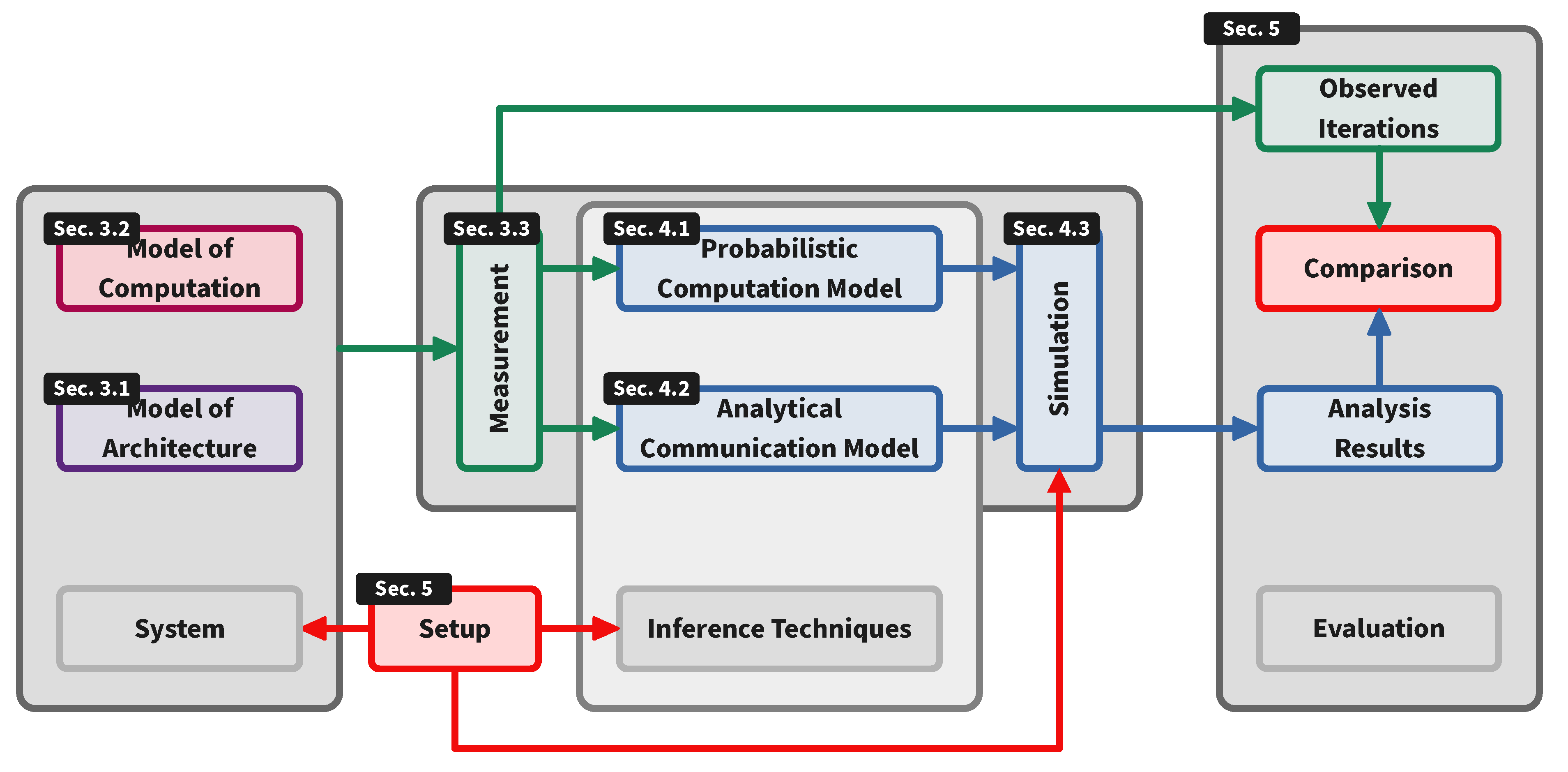
3. Workflow and Preliminaries
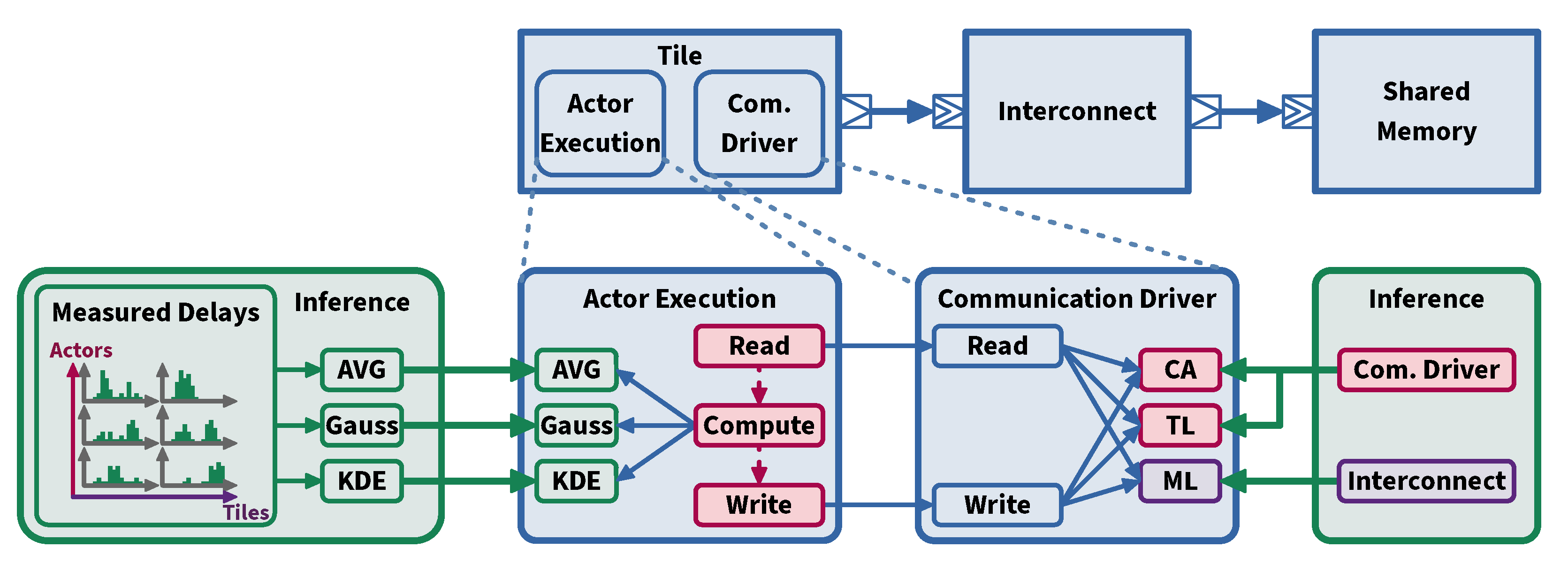
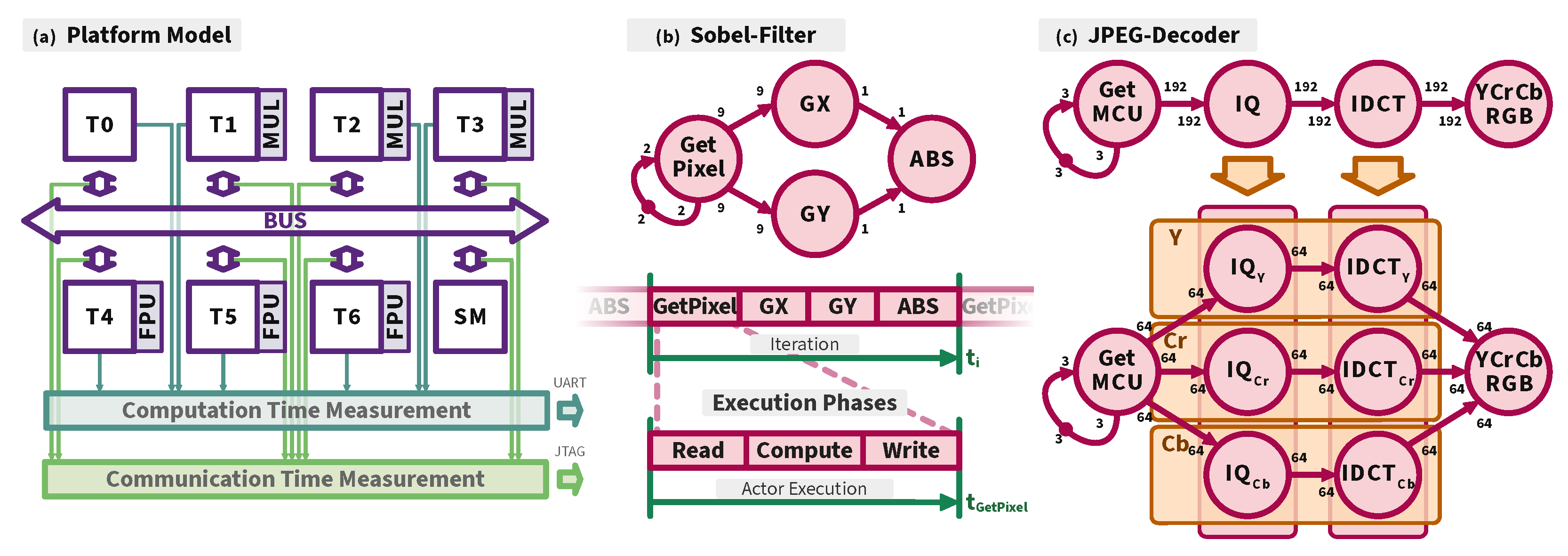
3.1. Model of Architecture (MoA)
3.2. Model of Computation (MoC)
3.3. Measurement Infrastructure
4. Computation and Communication Performance Modeling Approaches
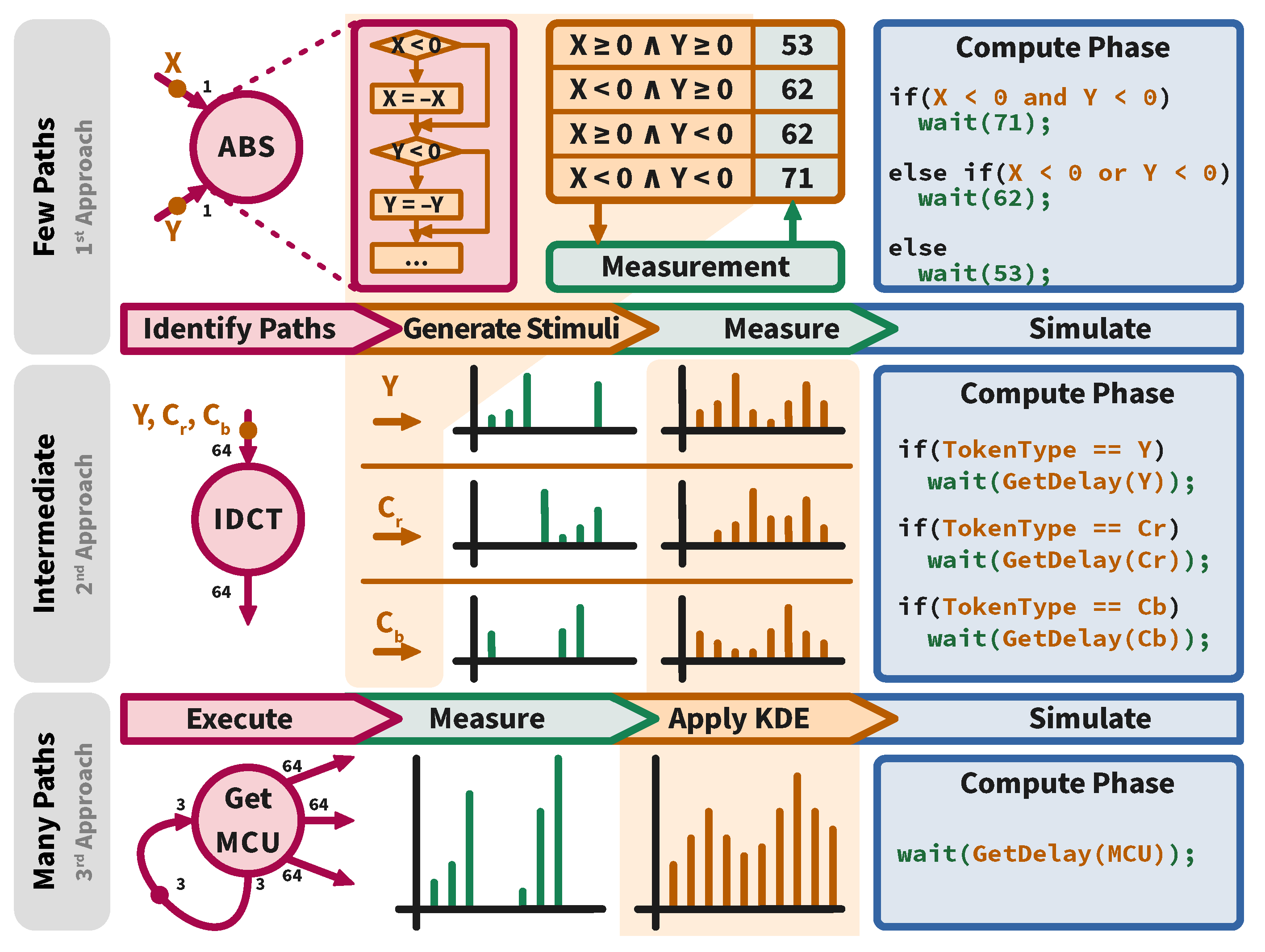
4.1. Computation Modeling Approach
4.1.1. Compute Time Representation
4.1.2. Data Dependency Consideration
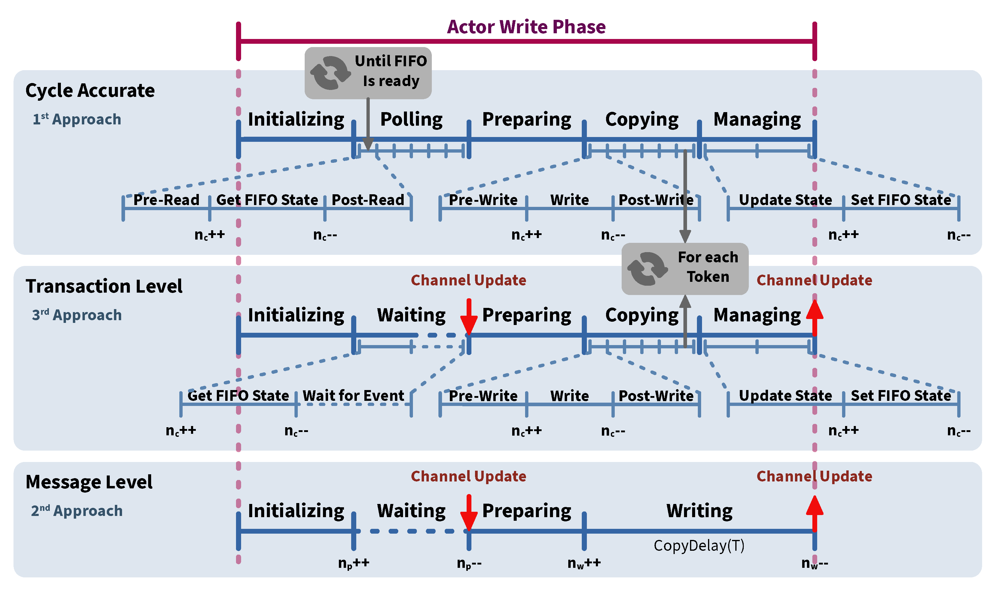
4.2. Communication Modeling Approach
4.2.1. Cycle Accurate Model
4.2.2. Message Level Model
4.2.3. Transaction Level Model
4.3. Simulation Model
5. Experiments
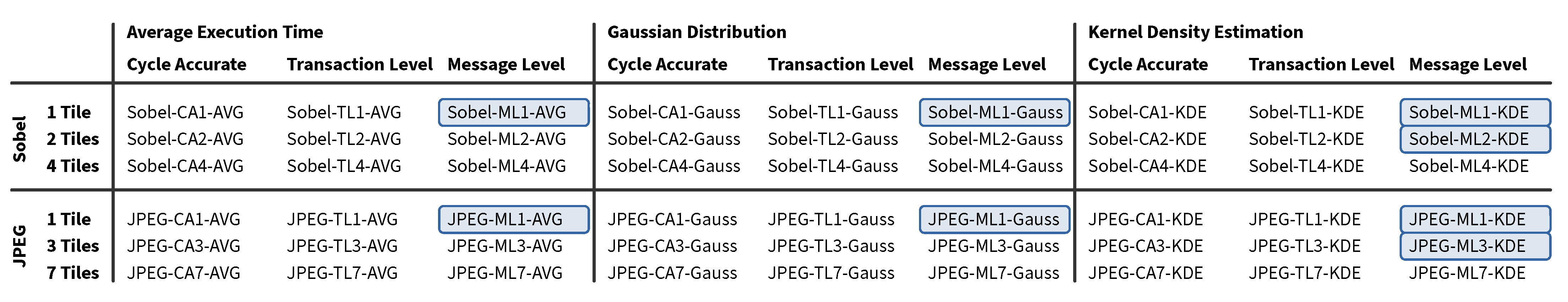
5.1. Experiment Setup
5.2. Use-Cases
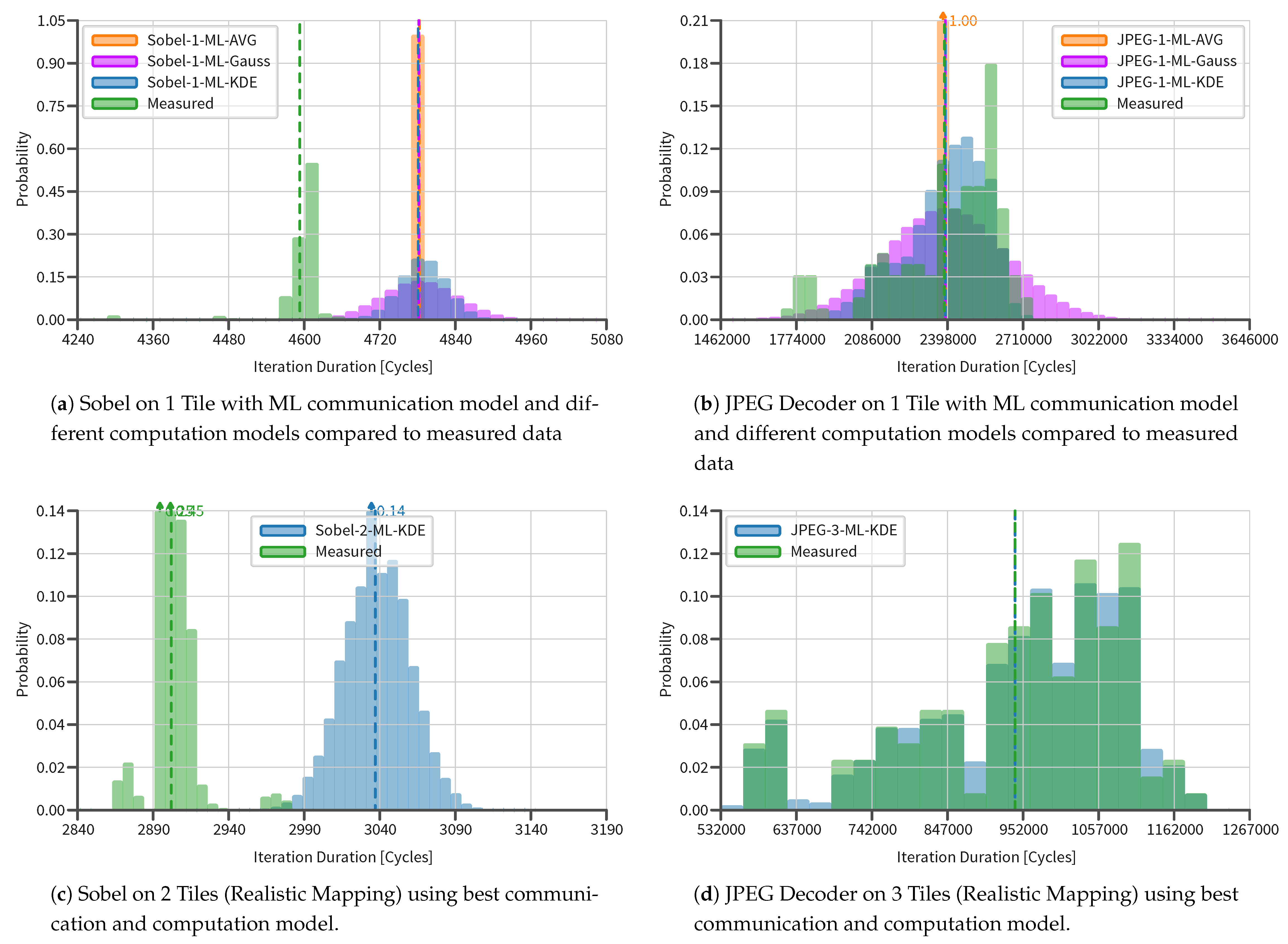
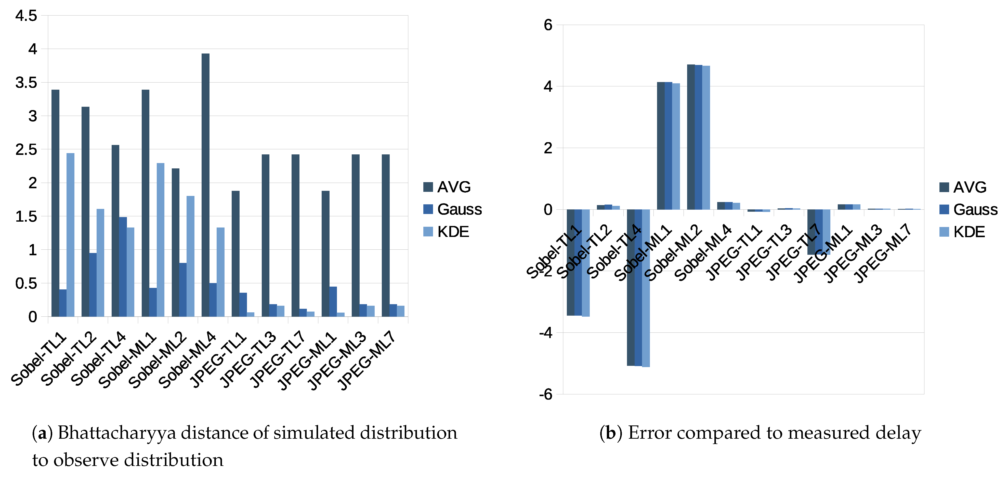
5.3. Results
5.4. Discussion
6. Future Work
7. Conclusions
Author Contributions
Funding
Data Availability Statement
Conflicts of Interest
References
- Gerstlauer, A.; Haubelt, C.; Pimentel, A.D.; Stefanov, T.P.; Gajski, D.D.; Teich, J. Electronic System-Level Synthesis Methodologies. IEEE Trans. Comput. Aided Des. Integr. Circuits Syst. 2009, 28, 1517–1530. [Google Scholar] [CrossRef] [Green Version]
- Stemmer, R.; Vu, H.D.; Grüttner, K.; Le Nours, S.; Nebel, W.; Pillement, S. Towards Probabilistic Timing Analysis for SDFGs on Tile Based Heterogeneous MPSoCs. In Proceedings of the 10th European Congress on Embedded Real Time Software and Systems, Toulouse, France, 29–31 January 2020; p. 59. [Google Scholar]
- Rosenblatt, M. Remarks on Some Nonparametric Estimates of a Density Function. Ann. Math. Statist. 1956, 27, 832–837. [Google Scholar] [CrossRef]
- Parzen, E. On Estimation of a Probability Density Function and Mode. Ann. Math. Statist. 1962, 33, 1065–1076. [Google Scholar] [CrossRef]
- Stemmer, R.; Vu, H.D.; Grüttner, K.; Le Nours, S.; Nebel, W.; Pillement, S. Experimental Evaluation of Probabilistic Execution-Time Modeling and Analysis Methods for SDF Applications on MPSoCs. In Proceedings of the 2019 International Conference on Embedded Computer Systems: Architectures, Modeling, and Simulation (SAMOS), Samos, Greece, 7–11 July 2019; pp. 241–254. [Google Scholar]
- Vu, H.D.; Le Nours, S.; Pillement, S.; Stemmer, R.; Grüettner, K. A Fast Yet Accurate Message-level Communication Bus Model for Timing Prediction of SDFGs on MPSoC. In Proceedings of the Asia and South Pacific Design Automation Conference, Online, 18–21 January 2021; p. 1183. [Google Scholar]
- Intel. Intel CoFluent Studio. Available online: https://www.intel.com/content/www/us/en/cofluent/cofluent-studio.html (accessed on 20 July 2021).
- Timing-Architect. Available online: http://www.timing-architects.com (accessed on 20 July 2021).
- ChronSIM. Available online: http://www.inchron.com/tool-suite/chronsim.html (accessed on 20 July 2021).
- SpaceCoDesign. Available online: www.spacecodesign.com (accessed on 20 July 2021).
- IEEE Standards Association. IEEE Standard for Standard SystemC Language Reference Manual; IEEE Computer Society: Washington, DC, USA, 2012. [Google Scholar]
- Kreku, J.; Hoppari, M.; Kestilä, T.; Qu, Y.; Soininen, J.; Andersson, P.; Tiensyrjä, K. Combining UML2 Application and SystemC Platform Modelling for Performance Evaluation of Real-Time Embedded Systems. EURASIP J. Embed. Syst. 2008. [Google Scholar] [CrossRef] [Green Version]
- Pimentel, A.D.; Thompson, M.; Polstra, S.; Erbas, C. Calibration of Abstract Performance Models for System-Level Design Space Exploration. J. Signal Process. Syst. 2008, 50, 99–114. [Google Scholar] [CrossRef] [Green Version]
- Pimentel, A.D.; Erbas, C.; Polstra, S. A systematic approach to exploring embedded system architectures at multiple abstraction levels. IEEE Trans. Comput. 2006, 55, 99–112. [Google Scholar] [CrossRef]
- Nouri, A.; Bozga, M.; Moinos, A.; Legay, A.; Bensalem, S. Building faithful high-level models and performance evaluation of manycore embedded systems. In Proceedings of the ACM/IEEE International Conference on Formal Methods and Models for Codesign, Lausanne, Switzerland, 19–21 October 2014. [Google Scholar]
- Le Boudec, J.Y. Performance Evaluation of Computer and Communication Systems; EPFL Press: Lausanne, Switzerland, 2010. [Google Scholar]
- Bobrek, A.; Paul, J.M.; Thomas, D.E. Stochastic Contention Level Simulation for Single-Chip Heterogeneous Multiprocessors. IEEE Trans. Comput. 2010, 59, 1402–1418. [Google Scholar] [CrossRef]
- Lu, K.; Müller-Gritschneder, D.; Schlichtmann, U. Analytical timing estimation for temporally decoupled TLMs considering resource conflicts. In Proceedings of theDesign, Automation Test in Europe Conference Exhibition (DATE), Grenoble, France, 18–22 March 2013; pp. 1161–1166. [Google Scholar]
- Chen, S.; Chen, C.; Tsay, R. An activity-sensitive contention delay model for highly efficient deterministic full-system simulations. In Proceedings of the Design, Automation Test in Europe Conference Exhibition (DATE), Dresden, Germany, 24–28 March 2014; pp. 1–6. [Google Scholar]
- Castrillon, J.; Velasquez, R.; Stulova, A.; Sheng, W.; Ceng, J.; Leupers, R.; Ascheid, G.; Meyr, H. Trace-Based KPN Composability Analysis for Mapping Simultaneous Applications to MPSoC Platforms. In Proceedings of the Design, Automation and Test in Europe, European Design and Automation Association, Dresden, Germany, 8–12 March 2010; pp. 753–758. [Google Scholar]
- Castrillon, J.; Leupers, R.; Ascheid, G. MAPS: Mapping Concurrent Dataflow Applications to Heterogeneous MPSoCs. IEEE Trans. Ind. Inform. 2013, 9, 527–545. [Google Scholar] [CrossRef]
- Michalska, M.; Casale-Brunet, S.; Bezati, E.; Mattavelli, M. High-Precision Performance Estimation for the Design Space Exploration of Dynamic Dataflow Programs. IEEE Trans. Multi-Scale Comput. Syst. 2018, 4, 127–140. [Google Scholar] [CrossRef]
- Bringmann, O.; Ecker, W.; Gerstlauer, A.; Goyal, A.; Mueller-Gritschneder, D.; Sasidharan, P.; Singh, S. The next generation of virtual prototyping: Ultra-fast yet accurate simulation of HW/SW systems. In Proceedings of the Design, Automation Test in Europe Conference Exhibition (DATE), Grenoble, France, 9–13 March 2015; pp. 1698–1707. [Google Scholar]
- Lee, E.A.; Messerschmitt, D.G. Synchronous data flow. Proc. IEEE 1987, 75, 1235–1245. [Google Scholar] [CrossRef]
- Geilen, M.; Basten, T.; Stuijk, S. Minimising buffer requirements of synchronous dataflow graphs with model checking. In Proceedings of the 42nd Design Automation Conference, Anaheim, CA, USA, 13–17 June 2005; pp. 819–824. [Google Scholar]
- Bhattacharyya, S.S.; Lee, E.A. Scheduling synchronous dataflow graphs for efficient looping. J. VLSI Signal Process. Syst. Signal Image Video Technol. 1993, 6, 271–288. [Google Scholar] [CrossRef]
- Schlaak, C.; Fakih, M.; Stemmer, R. Power and Execution Time Measurement Methodology for SDF Applications on FPGA-based MPSoCs. arXiv 2017, arXiv:1701.03709. [Google Scholar]
- AMBA® AXI™ and ACE™ Protocol Specification AXI3, AXI4, and AXI4-Lite ACE and ACE-Lite. Available online: https://developer.arm.com/documentation/ihi0022/e/ (accessed on 20 July 2021).
- Pedregosa, F.; Varoquaux, G.; Gramfort, A.; Michel, V.; Thirion, B.; Grisel, O.; Blondel, M.; Prettenhofer, P.; Weiss, R.; Dubourg, V.; et al. Scikit-learn: Machine Learning in Python. J. Mach. Learn. Res. 2011, 12, 2825–2830. [Google Scholar]
- Baccelli, F.; Cohen, G.; Olsder, G.; Quadrat, J. Synchronization and Linearity, an Algebra for Discrete Event Systems; Wiley & Sons Ltd: New York, NY, USA, 1992. [Google Scholar]
- Bhattacharyya, A. On a measure of divergence between two statistical populations defined by their probability distributions. Bull. Calcutta Math. Soc. 1943, 35, 99–109. [Google Scholar]


| Experiment→ | Jpeg-1 | Jpeg-3 | Jpeg-7 | Exp. → | Sobel-1 | Sobel-2 | Sobel-4 |
|---|---|---|---|---|---|---|---|
| Actor ↓ | Actor ↓ | ||||||
| Get MCU | 0 | 0 | 0 | GetPixel | 0 | 1 | 1 |
| 0 | 1 | 1 | GX | 0 | 2 | 2 | |
| 0 | 1 | 2 | GY | 0 | 1 | 3 | |
| 0 | 1 | 3 | ABS | 0 | 2 | 0 | |
| 0 | 4 | 4 | |||||
| 0 | 4 | 5 | |||||
| 0 | 4 | 6 | |||||
| YCrCb RGB | 0 | 0 | 0 |
| Experiment | Measured | Average | Gaussian | KDE | |||
|---|---|---|---|---|---|---|---|
| Sobel-CA1 | 4593.26 | 4445.00 | (−3.23%, 3.388) | 4444.84 | (−3.23%, 0.436) | 4443.33 | (−3.26%, 2.007) |
| Sobel-TL1 | 4593.26 | 4435.00 | (−3.45%, 3.388) | 4434.84 | (−3.45%, 0.404) | 4433.32 | (−3.48%, 2.442) |
| Sobel-ML1 | 4593.26 | 4783.00 | (4.13%, 3.388) | 4782.84 | (4.13%, 0.428) | 4781.33 | (4.09%, 2.291) |
| Sobel-CA2 | 2902.53 | 3100.00 | (6.80%, 2.210) | 3092.60 | (6.55%, 0.825) | 3091.98 | (6.53%, 1.941) |
| Sobel-TL2 | 2902.53 | 2907.00 | (0.14%, 3.134) | 2906.79 | (0.15%, 0.947) | 2905.78 | (0.11%, 1.607) |
| Sobel-ML2 | 2902.53 | 3039.00 | (4.70%, 2.212) | 3038.79 | (4.69%, 0.802) | 3037.78 | (4.66%, 1.800) |
| Sobel-CA4 | 3097.43 | 4623.00 | (49.25%, 2.665) | 4636.61 | (49.69%, 2.528) | 4639.62 | (49.79%, 4.891) |
| Sobel-TL4 | 3097.43 | 2939.99 | (−5.08%, 2.564) | 2939.79 | (−5.09%, 1.487) | 2938.78 | (−5.12%, 1.330) |
| Sobel-ML4 | 3097.43 | 3105.00 | (0.24%, 3.927) | 3104.80 | (0.24%, 0.502) | 3103.78 | (0.21%, 1.330) |
| JPEG-CA1 | 2,385,860.12 | 2,384,114.00 | (−0.07%, 1.877) | 2,384,156.45 | (−0.07%, 0.354) | 2,384,088.70 | (−0.07%, 0.061) |
| JPEG-TL1 | 2,385,860.12 | 2,384,094.00 | (−0.07%, 1.877) | 2,384,136.45 | (−0.07%, 0.354) | 2,384,068.00 | (−0.08%, 0.061) |
| JPEG-ML1 | 2,385,860.12 | 2,389,605.00 | (0.16%, 1.877) | 2,389,647.45 | (0.16%, 0.445) | 2,389,579.70 | (0.16%, 0.059) |
| JPEG-CA3 | 940,836.44 | 955,621.41 | (1.57%, 2.422) | 955,688.20 | (0.12%, 0.115) | 955,623.81 | (1.57%, 0.071) |
| JPEG-TL3 | 940,836.44 | 941,122.00 | (0.03%, 2.422) | 941,190.64 | (0.04%, 0.185) | 941,115.53 | (0.03%, 0.161) |
| JPEG-ML3 | 940,836.44 | 941,004.00 | (0.02%, 2.422) | 941,068.01 | (0.02%, 0.185) | 940,992.80 | (0.02%, 0.162) |
| JPEG-CA7 | 941,059.40 | 1,071,080.02 | (13.82%, 2.420) | 1,071,133.51 | (13.82%, 0.185) | 1,071,073.86 | (13.82%, 0.198) |
| JPEG-TL7 | 941,059.40 | 927,239.00 | (−1.47%, 2.422) | 927,303.56 | (−1.46%, 0.114) | 927,235.61 | (−1.47%, 0.075) |
| JPEG-ML7 | 941,059.40 | 941,170.91 | (0.01%, 2.422) | 941,234.74 | (0.02%, 0.184) | 941,160.56 | (0.01%, 0.160) |
| Experiment | Measured | CA Model | TL Model | ML Model | TL/ML Speed-up | |||
|---|---|---|---|---|---|---|---|---|
| Sobel-1-KDE | 0:07:40 | 0:03:12 | (2.40) | 0:03:04 | (2.50) | 0:01:44 | (4.42) | 1.77 |
| Sobel-2-KDE | 0:07:03 | 0:12:32 | (0.56) | 0:05:05 | (1.39) | 0:02:11 | (3.23) | 2.33 |
| Sobel-4-KDE | 0:07:13 | 0:20:00 | (0.36) | 0:05:21 | (1.35) | 0:02:18 | (3.14) | 2.33 |
| Jpeg-1-KDE | 13:14:31 | 0:52:29 | (15.14) | 0:51:35 | (15.40) | 0:19:03 | (41.71) | 2.71 |
| Jpeg-3-KDE | 5:12:58 | 67:31:00 | (0.08) | 1:20:56 | (3.87) | 0:23:41 | (13.22) | 3.42 |
| Jpeg-7-KDE | 5:13:02 | 56:19:42 | (0.10) | 1:20:57 | (3.87) | 0:25:29 | (12.28) | 3.18 |
Publisher’s Note: MDPI stays neutral with regard to jurisdictional claims in published maps and institutional affiliations. |
© 2021 by the authors. Licensee MDPI, Basel, Switzerland. This article is an open access article distributed under the terms and conditions of the Creative Commons Attribution (CC BY) license (https://creativecommons.org/licenses/by/4.0/).
Share and Cite
Stemmer, R.; Vu, H.-D.; Le Nours, S.; Grüttner, K.; Pillement, S.; Nebel, W. A Measurement-Based Message-Level Timing Prediction Approach for Data-Dependent SDFGs on Tile-Based Heterogeneous MPSoCs. Appl. Sci. 2021, 11, 6649. https://doi.org/10.3390/app11146649
Stemmer R, Vu H-D, Le Nours S, Grüttner K, Pillement S, Nebel W. A Measurement-Based Message-Level Timing Prediction Approach for Data-Dependent SDFGs on Tile-Based Heterogeneous MPSoCs. Applied Sciences. 2021; 11(14):6649. https://doi.org/10.3390/app11146649
Chicago/Turabian StyleStemmer, Ralf, Hai-Dang Vu, Sébastien Le Nours, Kim Grüttner, Sébastien Pillement, and Wolfgang Nebel. 2021. "A Measurement-Based Message-Level Timing Prediction Approach for Data-Dependent SDFGs on Tile-Based Heterogeneous MPSoCs" Applied Sciences 11, no. 14: 6649. https://doi.org/10.3390/app11146649
APA StyleStemmer, R., Vu, H.-D., Le Nours, S., Grüttner, K., Pillement, S., & Nebel, W. (2021). A Measurement-Based Message-Level Timing Prediction Approach for Data-Dependent SDFGs on Tile-Based Heterogeneous MPSoCs. Applied Sciences, 11(14), 6649. https://doi.org/10.3390/app11146649