Detection and Model of Thermal Traces Left after Aggressive Behavior of Laboratory Rodents

Abstract

Automation of complex social behavior analysis of experimental animals would allow for faster, more accurate and reliable research results in many biological, pharmacological, and medical fields. However, there are behaviors that are not only difficult to detect for the computer, but also for the human observer. Here, we present an analysis of the method for identifying aggressive behavior in thermal images by detecting traces of saliva left on the animals’ fur after a bite, nape attack, or grooming. We have checked the detection capabilities using simulations of social test conditions inspired by real observations and measurements. Detection of simulated traces different in size and temperature on single original frame revealed the dependence of the parameters of commonly used corner detectors (R score, ranking) on the parameters of the traces. We have also simulated temperature of saliva changes in time and proved that the detection time does not affect the correctness of the approximation of the observed process. Furthermore, tracking the dynamics of temperature changes of these traces allows to conclude about the exact moment of the aggressive action. In conclusion, the proposed algorithm together with thermal imaging provides additional data necessary to automate the analysis of social behavior in rodents.

1. Introduction

Laborator animal behavior analysis is an issue of great value in such research branches as medicine, pharmacology, biology, or neuroscience. The most commonly used species of laboratory animals are rodents, whose wide range of social interactions enables conducting researches on neurological diseases, social dysfunctions, drug discovery, or brain functioning. To produce reliable data, analysis of the social behavior should be performed by an experienced annotator on the basis of careful observations of the test scene [1]. The problem, however, is the manual scoring, which is error-prone. Due to this limitation, researchers have proposed different solutions for automation of animal behavior analysis. The most common approach is to distinguish behavior on the basis of the mutual position and the body displacement [2,3]. Other systems additionally track different key points like nose, snout, or a base of the tail [4]. Few studies have been adopting statistical measures for trajectory analysis [5,6,7]. Another solution uses detailed ethograms in combination with multivariate approach known as T-pattern analysis [8].

Recently, there is a great interest in using machine learning and neural networks to understand social behavior [9,10,11]. Lorbach in [12] presents a rat social interaction dataset with results of using it as a training set for a method of recognizing interactions with rats. The solution proposed in [13] detects attack, mounting, and close interaction between two mice with different coat colors. Twenty-seven features were extracted from images obtained from a traditional video camera as well as from depth camera to train the random model. The work in [14] describes the fine-tuning method of a pre-trained convolutional neural network only for the recognition of exploration behavior. Crispim et al. [15], in turn, present a method for behavior identification (locomotion, immobility, rearing, and grooming) using multilayer perceptron networks. The authors claim that for proper recognition of various behavior, training should be based on two types of input parameters: morphological (e.g., animal’s body area or length) and kinematic (e.g., the distance traveled). They also proved that statistically-guided input feature selection significantly improves the classification performance.

However, very often these machine learning-based solutions give results similar to simpler methods. This can suggest that learning-based algorithms require enriched information and it is necessary to use more various features. There are two different ways of enriching information.

The first one is more circumstantial feature detection. Parameters commonly used in the training phase are body size and location, speed of movement, and mutual orientation of animals. Based on the analysis of only these features, it is possible to create system that can recognize general behaviors like grooming, exploration, chase, or approach. To discern between more complex social behaviors, e.g., bite attack or social grooming, there is, however, a need for detailed information about animals. Tracking certain regions of interest like the snout or base of the tail is rare [12,16] but valuable for behavior recognition.

The second method of enriching input information is to use various data acquisition and processing techniques and technologies. Some of the above-mentioned methods use statistics to reveal and describe sequences of behavior [8], others have extended the usual morphological feature set with kinematic [2,15] or 3D (depth) features [13,16]. There are also systems that use thermal technology to obtain new information [3,17,18].

One of the biggest advantages of thermal recordings in animal studies is undoubtedly the limitation of stress caused by artificial lighting required for recordings with visible light cameras. Many social behaviors of nocturnal animals are not possible in the strong light. Another benefit is the image of heat distribution. The value and dynamics of body temperature can visualize different physiological processes and may indicate the occurrence of behaviors such as fear or stress [19,20]. Finally, the warmth distribution can also be an individual identifier [21].

Another, less frequently used advantage of thermal imaging is the possibility of observing phenomena that are beyond human natural perception. Therefore, thermal imaging is a great tool for visualizing areas not available in visible-light imaging. Examples of such areas include water or saliva traces on an animal’s fur, body regions with higher temperature values (e.g., due to more intensive thermoregulation processes), etc.

The human eye, unlike the thermal camera, is unable to spot the trace of water or saliva applied on the rodent’s fur, and the trace of saliva can be the only evidence of a bite or social grooming event occurrence [18].

Crucial information for behavior recognition is a pose estimation, which involves an assessment of the geometrical configuration of the body parts. Tracking certain body parts has been shown to improve behavior recognition [22]. Lorbach and others proved in [23] that precise localization of body parts is beneficial for recognizing interactions described by a specific pose. They have examined the impact of animal misidentification and errors due to inaccurate localization of the interesting points. Incorrect tracking of three points (the nose, the center of gravity, and the tail-base) turned out to have a huge impact on the operation of the six off-the-shelf classifiers during the recognition of eight animal behaviors. They also pointed out that there do exist some unresolved confusion that persists even with perfect tracking. Some behaviors are very ambiguous in their appearance (for example, allogrooming, nape attacking, pinning, and social nose contact) and thus the classifier needs more data or features to separate classes properly. The main conclusion from this work emphasizes that feature quality, rather than classifier, largely determines the algorithms’ performance.

Here, we show methods to support the automation of animal aggressive behavior analysis using thermal imaging techniques. In this paper, we have decided to propose data simulation methods, as it is very difficult to obtain real measurements with various properties of the animal behavior, their mutual interaction, and different parameters of saliva traces. We further used the simulated thermal sequences to do the following.

• Investigate the influence of corner detector parameters on the detection of interesting points related to saliva traces.
• Investigate the influence of the properties of the simulated saliva traces on the detection results.
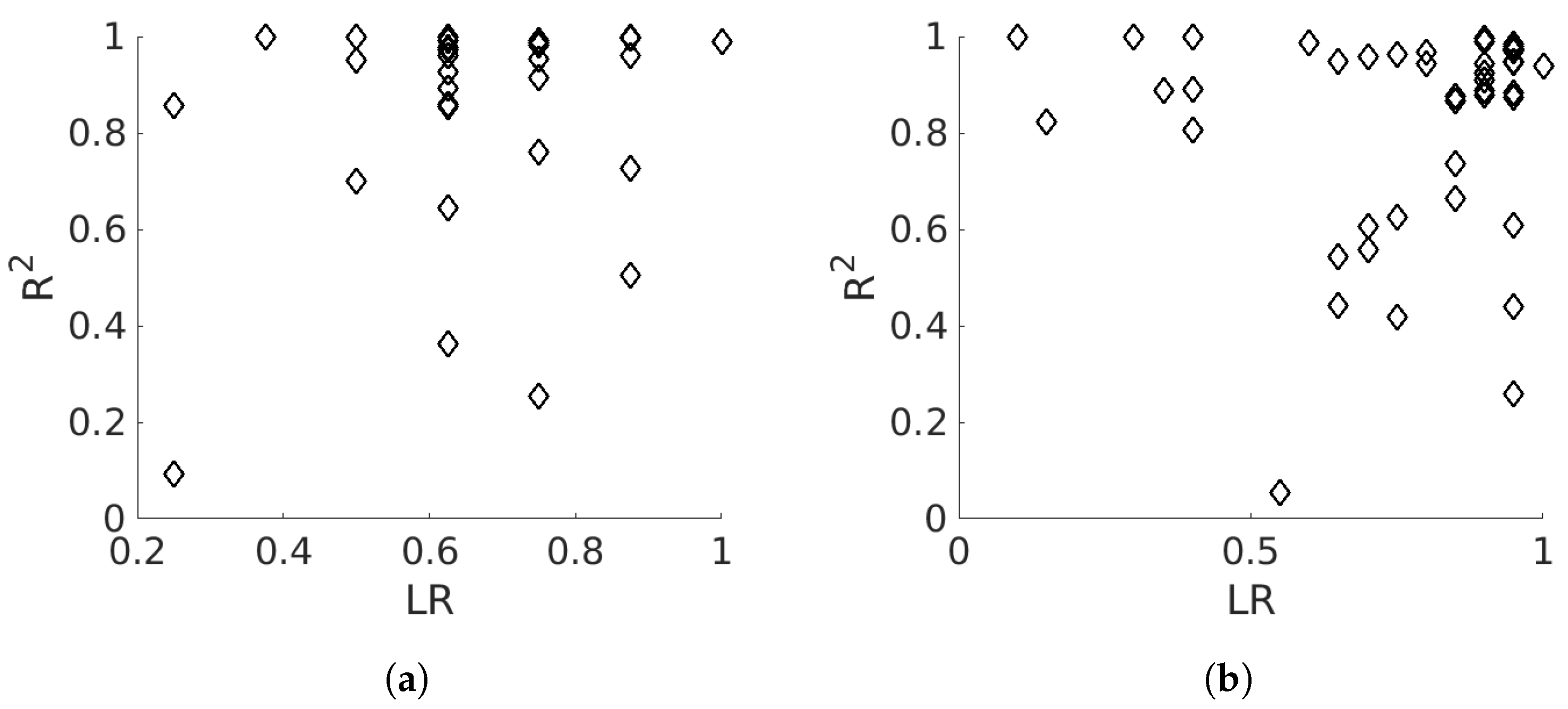
• Investigate the conditions when the cooling–heating model describing the temperature behavior of the saliva trace could be successfully fitted to the observable data.
• Answer the question if the cooling-heating model could be potentially used to estimate the exact bite time even, when the bite event is not directly recorded (e.g., as one animal covers another, due to the limited camera frame rate, etc.).

This paper is organized as follows. In Section 2, we describe the data used for the analysis: the measured thermal data (Section 2.1) on the basis of which simulations were created (Section 2.2). The research was divided into two parts: the static and temporal analysis. Section 3 describes the methodology of both those analysis separately. The experiment results are presented in Section 4 and discussed in Section 5. We conclude in Section 6.

2. Materials and Methods

For the purposes of the analysis, data were collected in the form of thermal sequences measured on animals during social testing, as well as in the form of simulated data.

2.1. Thermal Data Acquisition

Thermal sequences of the animal interactions were recorded during social tests [24]. A single test lasted 15 min and consisted of observing two adult male Wistar rats placed in a plexiglas cage. Image sequences were recorded using the FLIR A320G camera (FLIR Systems, Inc., Wilsonville, OR, USA) situated 120 cm above the cage with the spatial resolution of 320 × 240 pixels, 60 fps, and 16-bit image presentation. The animals were not illuminated. The whole thermal database consists of almost 300 min of recordings with 14 different individuals. All details about the database are presented in [18,25].

Animals bred, specifically for laboratory purposes, may have disturbed reactions that determine survival in the wild. This was observed during the recording of tests on a certain batch of rats. Sometimes they were not interested in establishing hierarchy and showed no aggressive behavior. To test proposed algorithms and solutions in fixed conditions, the data that can be adjusted were needed. For this purpose, we have created simulated data of animals test recording on the basis of which we can conclude about the detection results.

2.2. Data Simulation Methods

We have simulated shapes, the texture of the fur, animal motion, and bite marks left on the fur. Our goal was not to perfectly simulate kinematics or other parameters of the rodents, but to augment the image dataset used in the interesting points detection study. The controlled simulations allow obtaining images representing different scenarios important for further analysis.

2.2.1. Shape Simulation

The body shape has been simulated by four circles, the mutual positions of which were determined by certain relationships developed during animals observation in the laboratory. Figure 1 demonstrates examples of calculated objects with boundaries. The two largest inner circles form the body of the animal, the smaller outer circle is the head, and the smallest outer circle simulates the tail. After creating the general shape, tangents were defined for each of the two neighboring circles that marked the boundary of the object.

2.2.2. Texture Simulation

The simulation of the surface temperature distribution on an object is composed of two stages:

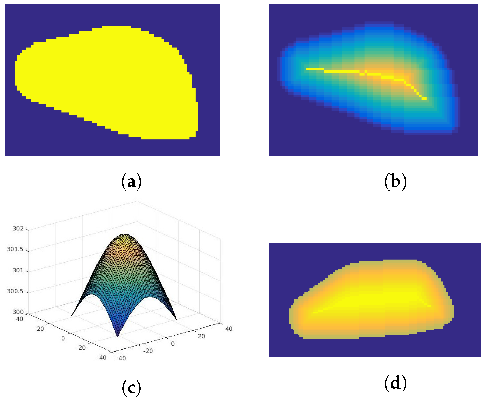
• Division of the area into subregions—uses skeletonization method based on the parallel thinning of the object described in [26]. This algorithm iteratively removes external pixels in such a way that the object (Figure 2a) shrinks to the middle line (dorsum). Figure 2b presents this method with each iteration marked with different color. The color is distributed linearly.
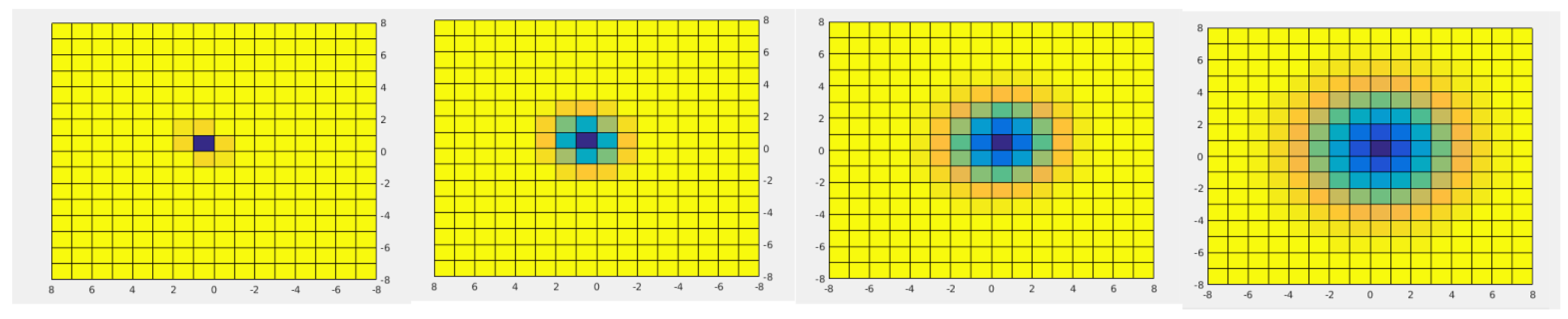
• Assigning temperature to each subregion—a process of sampling Gaussian distribution (Figure 2c) according to the number of iteration steps and normalization to the surface temperature of the body range. Each subsequent subdivision determined by the skeletonization algorithm is given the next temperature value according to the created distribution (Figure 2d). The degree of variability of the simulated texture can be adjusted by the value of the distribution variance.

Figure 2. Stages of texture simulation: (a) the initial shape, (b) shape after skeletonization with linear labeling of each iteration, (c) choosing the distribution for labeling, and (d) applying distribution to a thinned texture.

Figure 2. Stages of texture simulation: (a) the initial shape, (b) shape after skeletonization with linear labeling of each iteration, (c) choosing the distribution for labeling, and (d) applying distribution to a thinned texture.

Figure 2 presents the simulation of the body texture, in this particular case—simulation of the surface temperature distribution. This distribution is not equal in every part of the body. The highest temperature can be observed in the middle of the object (along the ridge), the lowest—near the object’s boundaries. The temperature changes gradually. The characteristic points of the body are places on the rodent body with a distinctly different temperature than the rest of the body area, like nose and eyes.The nose was simulated by a circular, low-temperature gradient, and the eyes, in turn, by an ellipse with a gradient texture. Figure 3a,b presents the images after applying the characteristic points on the calculated texture.

2.2.3. Motion Simulation

The motion of the shape in the $t+1$ frame is calculated based on the head direction relative to the front part of the body in t frame. In practice, the body follows the head. The position of the head at time $t+1$ is randomly chosen in the specified range around the body.

A simulation of two consecutive frames of two rats in the cage is shown in Figure 3 (Figure 3b follows Figure 3a). Figure 3a,d presents the position of the body in $t+1$ frame (unfilled circles) that is calculated based on its position in t frame (filled circles). Both shapes are calculated independently of each other according to the previously presented relations between circles and successive frames. Those shapes are then transferred into one image, and intersections are detected. During the recordings, animal bodies have been overlapping each other as a result of, e.g., climbing or offensive position, therefore, in the simulations, collisions, and intersections of objects are allowed.

2.2.4. Bite Event Simulation

The traces of saliva are randomly placed on the body when the intersection of the snout of one individual and the body of another appears (Figure 3a,b). In the following frames, the mark must still be in the same place on the body, so its position is calculated according to the rules described in Section 2.2.3. During the overlap, the underlying object is not visible, as well as all its bite marks. Fading of the trace is simulated by a sudden drop and then gradual increase in temperature in subsequent frames according to the results in [25] shown in Figure 4.

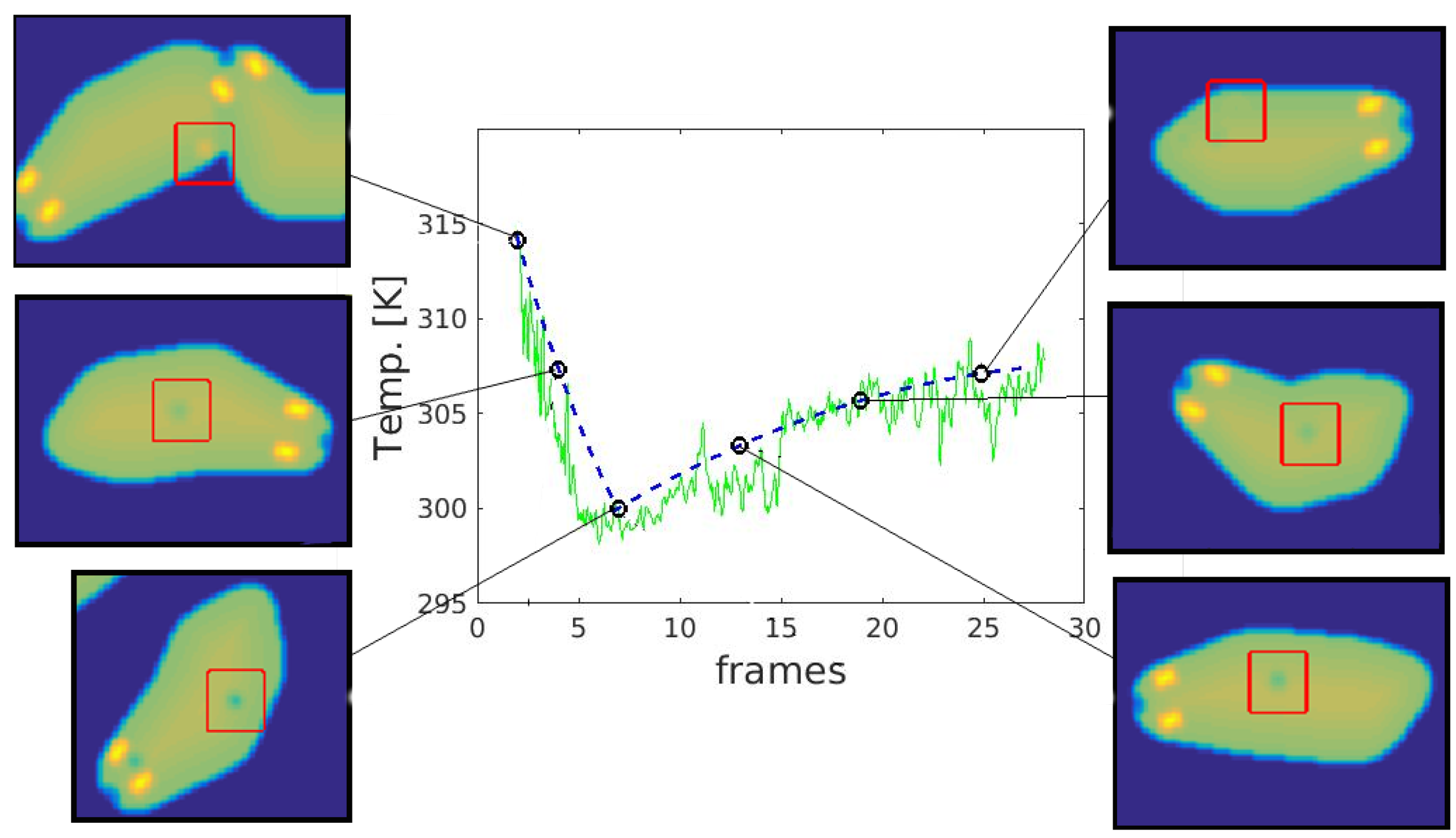
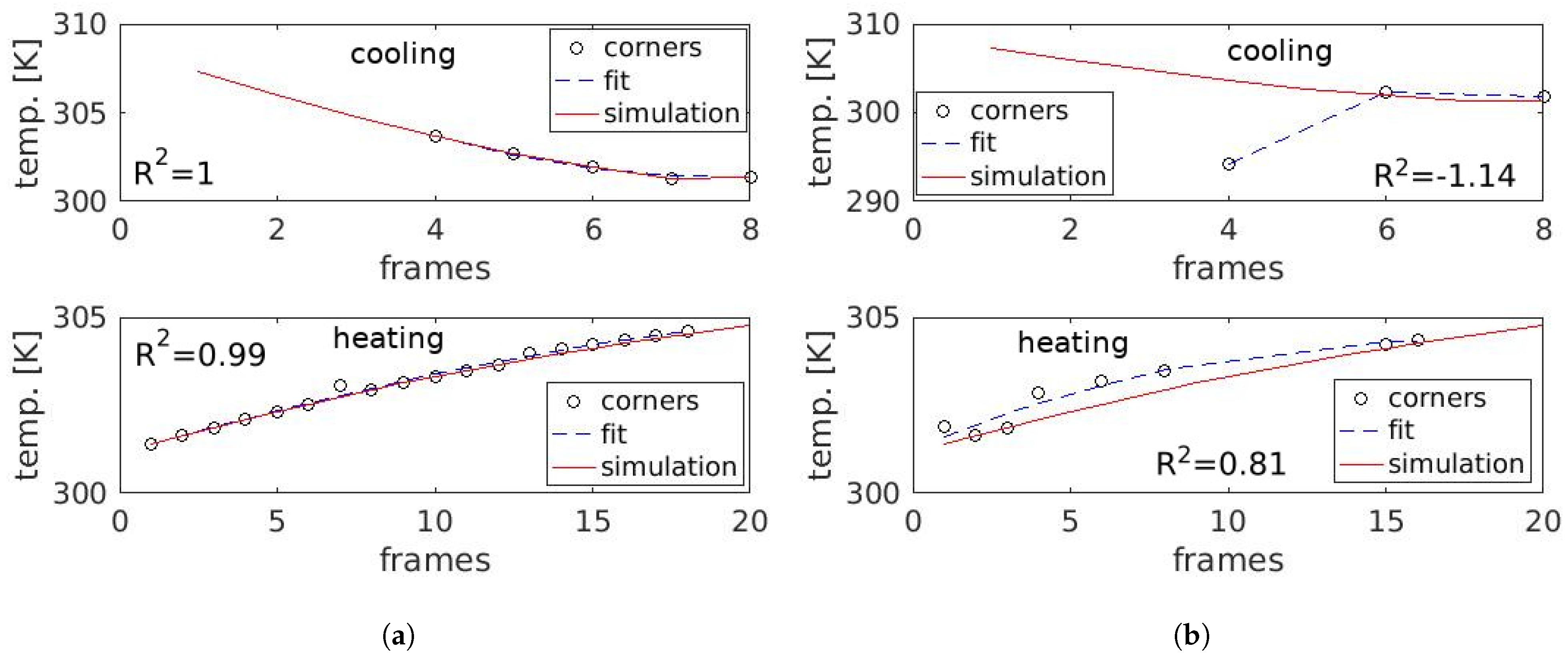
2.2.5. Temporal Changes Simulation

The trace of saliva, however, unlike other characteristic points on the body, has fluctuating temperatures and eventually dries up. A relatively small increase in body surface temperature could introduce significant changes in quality of the interesting point detection [18]. The observation of temporal changes in a saliva trace on a rodent’s fur could be modeled by two separate processes that affect the traces [25] (see Figure 4—green line):

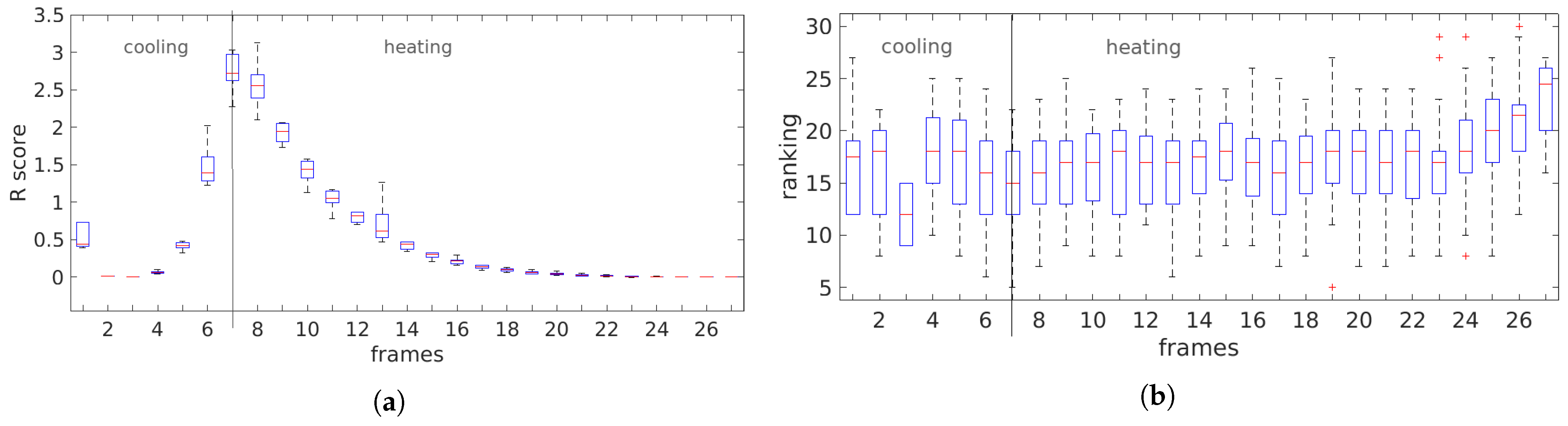
• cooling—very short and often unnoticeable, associated with the rapid heat dissipation by the liquid;
• heating—long-lasting temperature increase up to the ambient temperature caused by the drying, results in a gradual deterioration of visibility until the trace disappears completely.

Therefore, to investigate the influence of temporal changes in the saliva trace appearance and related performance of the interesting points detection we decided to introduce additional social test simulation.

The simulation of the trace dynamics consisted in marking the animal’s body with a trace that changed in time in accordance with the observations described in the [25]. All marks were in same size (2 px) and temperature (299 K). The introduced simulated temperature changes over time are presented in the graph in Figure 4 and marked using the blue dashed line. The green line shows an example of the measured temperature in time. Other measurements of temperature changes showed that the dynamics and visibility time of the traces are varied, but all measurements showed the best fit to the second order polynomial. During the simulation, the same temperature versus time function was used for all traces. Six selected frames in Figure 4 are illustrating the view of the simulated saliva traces on the animal’s body. At first, the temperature is high, higher than the surface of the body on which it is located and can be easily spotted as the bright yellow mark. However, then it drops quickly and turns blue in the image. This is followed by a slower drying process, in which the temperature of the trace rises to the temperature of the body surface and finally reaching the steady-state temperature before a bite. The boundaries of the traces have been blurred and adjusted to the body temperature to resemble natural marks as much as possible.

3. Data Analysis Methods

In this section, we present methods applied to real and simulated data to evaluate the influence of trace and corner detectors parameters on the detection results. We also investigate the possibilities of identifying trends in temperature changes of traces in simulations.

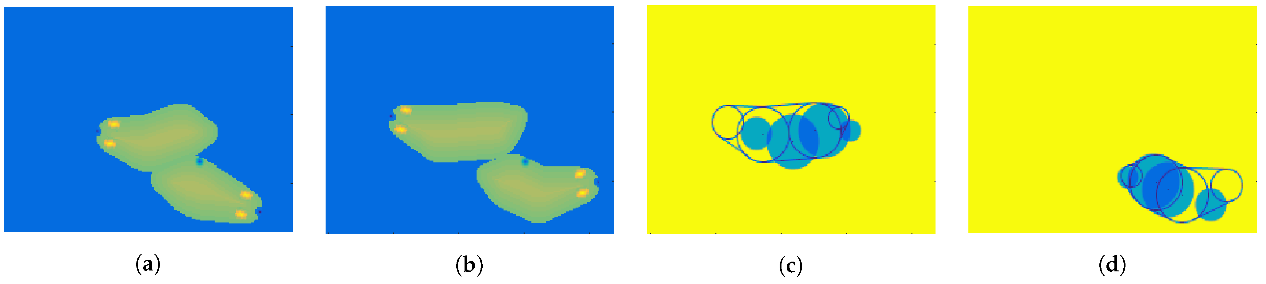
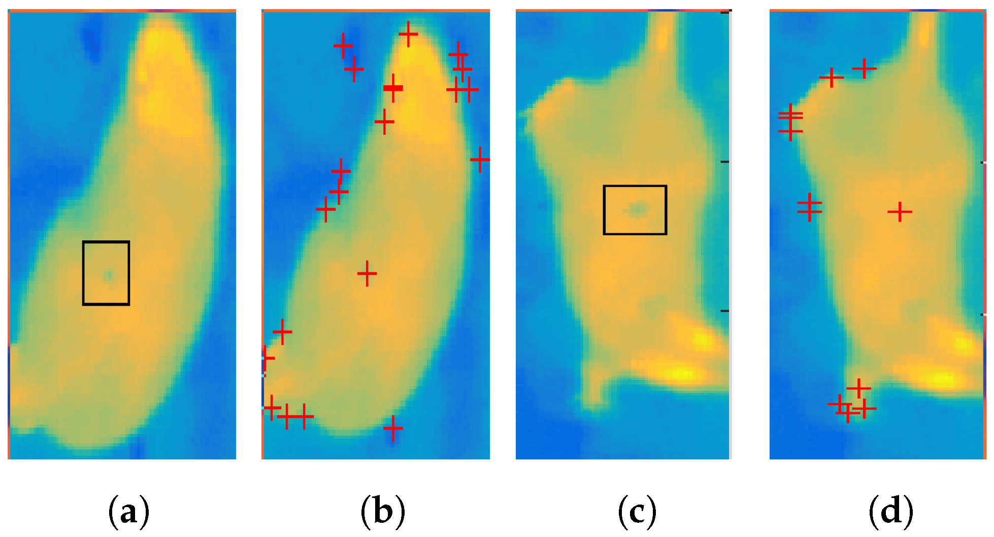
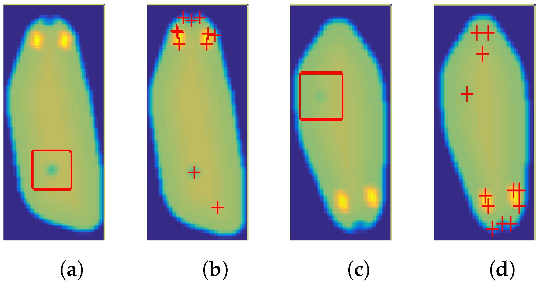
3.1. Corner Detection

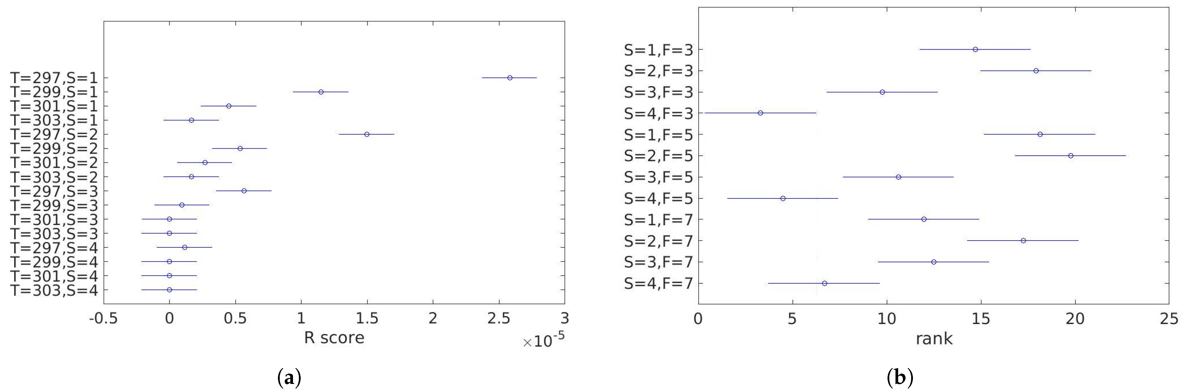
Analysis of behavior based on recordings is usually reduced to perceiving behaviors as a set of image features. The decision on the similarity of two behaviors is thus replaced with the appropriate detection and description of the set of features. Presentation of the image as parameters of selected regions or points turned out to be more effective in behavior recognition than presentation as parameters of the whole image [27].

There are many methods for detecting spatial points of interest described, for example, in [28]. Corner detectors find pixels with the largest variation in intensity in a neighborhood, that means points of a definitely different temperature than the surroundings—for thermal images. In our experiments, we have been using thermal images and tested three corner detectors: Harris [29], Shi-Tomasi [30], and FAST [31]. The preliminary results are described in [18].

Based on the previous experiments and other studies, we used two measures of point detection quality:

• the Corner Response Score (R score),
  for Harris detector defined as

  $$R={\lambda }_1{\lambda }_2-k{({\lambda }_1+{\lambda }_2)}^2$$

  (1)

  where
  ${\lambda }_1$ i ${\lambda }_2$—eigenvalues of the covariance matrix of the pixel intensity gradient,
  k—tunable sensitivity parameter.
• rank—the position on the list of corners sorted in a descending order by the R score.

All detectors were applied to the simulated static images of rodents with saliva traces and to the simulated images with temporal changes of saliva traces. The detected corners were not only the points of traces, but also other points with a large temperature gradient in the neighborhood. The method of identifying traces among all corners may use, e.g., tracking temperature changes in consecutive frames and is described in detail in the Section 3.3.

3.2. Static Analysis

The static approach was a simulation of saliva trace on the original, single image of the animal. Different simulations of traces were applied into the original images obtained from the camera. Traces differed in terms of

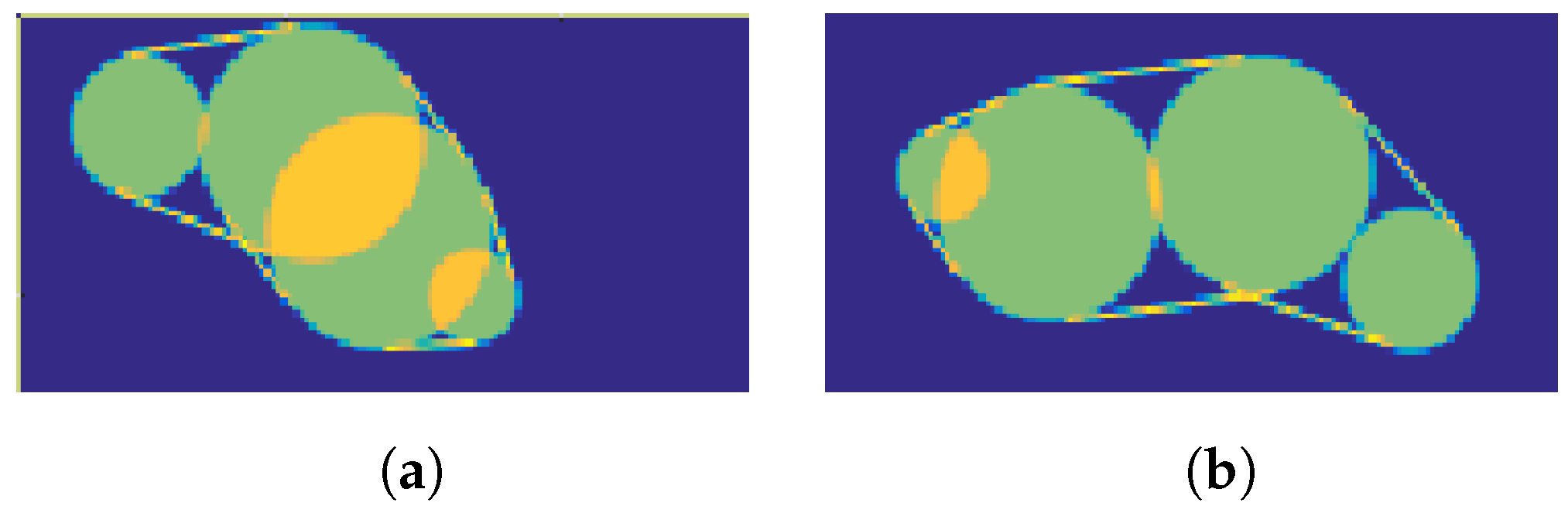
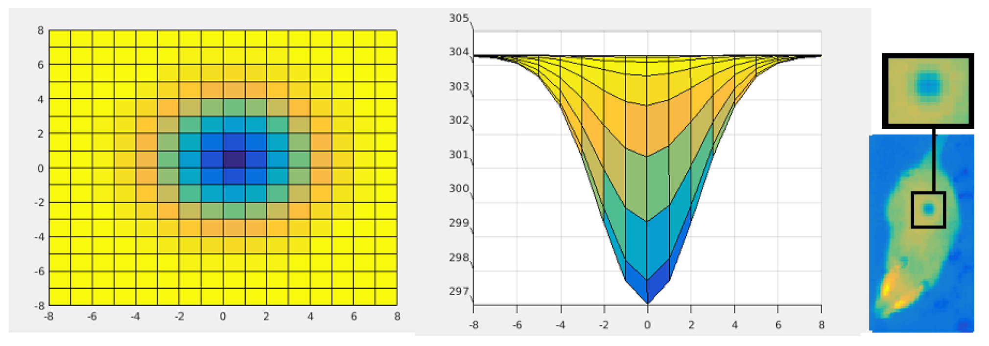
• temperature: 297, 299, 301, and 303 K (Figure 5),
• size and pixel intensity gradient—four stages (Figure 6): radius equal 1, 2, 3, or 4 pixels.

All the above parameters were proposed on the basis of observations in order to best reflect the actual traces. The simulated marks were of Gaussian distribution in both planes (Figure 7). Traces with greater variance were characterized by a larger size and a less steep slope (and thus a smaller gradient of pixel intensity in the neighborhood) than traces of smaller variance. Every circular trace had the same variance in both planes (Figure 6).

Harris and FAST detectors were used to detect simulated traces in real images. The Shi–Tomasi algorithm was not used in this analysis due to the results being very similar to the Harris algorithm [32]. Four different sizes of detector filters (3 × 3, 5 × 5, 7 × 7, and 9 × 9) were used to study the influence of detector parameters on the detection quality. The detectors were applied to the 400 simulated images representing 16 tested configurations of parameters: a combinations of 4 temperature values and 4 size of traces.

The rank and the R score calculated on the basis of Equation (1) for the Harris algorithm and the number of points satisfying the condition of the appropriate pixel intensity for the FAST algorithm [31] were adopted as quantitative parameters describing the detection.

3.3. Temporal Analysis

The goal of temporal analysis was the observation of interesting points temperature changes in time.

The Harris corner detector with a filter size equal 5 and a minimum accepted quality of corners set to 0.000001 was used for the simulated image sequences. The low accepted quality value requirement was caused by the lack of a clear trace border, which was neither observed in the real recordings. The final algorithm of identification saliva trace among all detected corners should include the following steps:

• computing the significance of corners using a specific measure, e.g., R score or ranking—rejection of irrelevant points,
• elimination of corners that do not meet certain conditions: e.g., temperature value within a certain range, location on the animal’s body, and
• prediction of trace localization based on the animal’s displacement vectors from previous frames.

Here, a simplified detection algorithm has been adopted, because the research is aimed at checking the possibility of finding the trend of temperature changes for incomplete observations and not the detection itself. The saliva trace detection in this work has the advantage that the exact location of the simulated trace is known. It consists in searching for a corner at a certain distance from the known simulation place. Setting the search area instead of the exact location of the trace allows for detection similar to the real one, when another point with a large gradient (object boundary, body parts with extreme temperature) located a close distance from the trace is detected with better score.

The generated traces of saliva were applied to the objects during movement simulation and, therefore, may be incomplete as a result of covering one body by another. Here, we introduce a length ratio (LR) which is defined as the ratio of the time period within which the saliva trace was detected to the time period when the saliva trace was simulated:

$$LR=\frac{\mathrm{time} \mathrm{period} \mathrm{of} \mathrm{the} \mathrm{detected} \mathrm{saliva} \mathrm{trace}}{\mathrm{time} \mathrm{period} \mathrm{of} \mathrm{the} \mathrm{simulated} \mathrm{saliva} \mathrm{trace}}$$

(2)

Here, both periods are measured in the number of frames. Time period of detected trace determines the time the trace was visible to the corner detector. The period of time for the simulated data is equal 27 frames (see Figure 4).

The bite action always takes place during close contact, and often the trace can be spotted only when animals move away from each other. This makes the exact moment of the bite very hard to notice when observing the interaction of animals in the visible light frequency. A fading trace of saliva left on the fur is an evidence of being bitten or groomed. The curve fitted to the corner temperature measurements would additionally allow to calculate the exact moment of these actions.

For each measurement of the detected corners we have applied the curve fitting procedure. It was followed by the coefficient of determination ($R^2$) calculation between the measures (fitted curve) and the simulated polynomial function.The definition of the coefficient of determination is

$$R^2=1-\frac{S{S}_{res}}{S{S}_{tot}}$$

(3)

where

$S{S}_{res}={\sum }_i{(y_i-f_i)}^2$ is the residual sum of squares,

$y_i$—measurements, $f_i$—modeled values,

$S{S}_{tot}={\sum }_i{(y_i-\overline{y})}^2$ is the total sum of squares,

$\overline{y}$—mean of the observed data.

We have also used the Pearson correlation coefficient to measure the linear correlation between the length of the trace and the fitting quality:

$$\rho =\frac{1}{N-1}\sum _{i=1}^N\left(\frac{\overline{y_i-{\mu }_y}}{{\sigma }_y}\right)\left(\frac{\overline{f_i-{\mu }_f}}{{\sigma }_f}\right)$$

(4)

where

N is the number of observations,

${\mu }_y$ and ${\sigma }_y$ are the mean and standard deviation of measurements,

${\mu }_f$ and ${\sigma }_f$ are the mean and standard deviation of the modeled values.

4. Results

4.1. Static Analysis

Table 1. The p-values of three-way ANOVA for the R score and the ranking for Harris and FAST algorithms. If the p-value is less than ${10}^{-17}$, it is replaced with 0 in the Table. Symbol (∗) denotes the results of interaction between factors.

	Harris		FAST
	R Score	Rank	R Score	Rank
temperature	0	0	0	0
size of a trace	0	0	0	0
filter size	0	0.1241	-	-
temperature ∗ size of a trace	0	0	0	0
temperature ∗ filter size	0	0.0023	-	-
size of a trace ∗ filter size	0	0.0165	-	-
temperature ∗ size of a trace ∗ filter size	0	0.3671	-	-

presents the results of three-way ANOVA to determine if the means of the R score and the ranking differ with respect to groups of three factors for the Harris detector (temperature, trace size, and filter size) and two factors for the FAST algorithm (temperature and the trace size). The FAST algorithm does not have a filter size parameter; therefore, this factor was not included in the ANOVA analysis for this detector. The p-values are presented in the table and the significance level was assumed as 0.05 (confidence level 95%).

An exemplary 2-factor comparisons are presented in Figure 8. Figure 8a shows the influence of temperature and the trace size on R score, while the dependence of the filter and trace size on the ranking is shown in Figure 8b.

Two exemplary images of simulated traces and results of Harris corner detector are presented in Figure 9.

4.2. Temporal Analysis

Figure 10 shows two simulated images with traces and the results of Harris detector. The simulated trace was superimposed on the simulated shape during simulated motion of two objects, therefore sometimes the trace was covered by the body of the other individual. A small proportion (7.6%) of all simulated trace sequences had only one measurement per process (the trace was visible for only one frame during whole process) and were therefore excluded from further analysis. Nearly one-fifth (18.9%) of cooling and 9.4% of heating processes achieved negative coefficient of determination value, indicating poor fitting of the data to the model. In fact, a negative result was often caused by one wrong measurement and/or a small number of all measurements (see Figure 11b cooling). The average length ratio LR for the rest of measurements was 0.44 ± 0.12 and 0.47 ± 0.25.

The mean values of coefficient of determination ($R^2$) between the observations and simulated values for the rest of traces was 0.87 ± 0.22 for cooling and 0.81 ± 0.23 for heating processes.

The effect of the trace length on the $R^2$ value was calculated using the correlation coefficient, which was equal to 0.15 for cooling and 0.08 for heating. The scatter plots for both processes are presented in Figure 12.

Figure 11 shows some curves fitted to the corners detected by the Harris algorithm. Black circles denote detected corners, and the blue dashed line is the curve best fitted to the observed corners. The red solid line presents the simulated (modeled) curve. The coefficient of determination presented for each process measures the quality of fitting the temperature of detected corners to the simulated data. We have chosen one example of a good fit (Figure 11a) and one example of a poor fitting (Figure 11b).

A visualization of summary statistics for the R score and the ranking grouped by the simulation frame number are presented in Figure 13 as a box plot. The bottom and the top of each box are the 25th and 75th percentiles of the sample, respectively. The red line inside each box is the sample median. The whiskers extend to the adjacent values, which correspond to approximately $\pm 2.7\sigma$. Observations beyond the whisker length are outliers marked as a red + sign only in Figure 13b. Outliers for R score were omitted in Figure 13a so as not to clutter the image.

5. Discussion

5.1. Static Analysis

The detection results are strongly dependent on the saliva trace parameters—temperature and size. This is confirmed by the results of the three-way ANOVA test presented in Table 1. The results for all factors as well as for the interaction between them allow us to reject the hypothesis that they do not influence the R score for both detectors. The p-value of 0.1241 indicates that the mean rankings for different Harris filter sizes are not significantly diverse. Similarly, the p-value of 0.3671 indicates that the mean rankings for interaction between all factors are not significantly different. However, p-values of 0.0023 and 0.0156 as well as 0 are small enough to conclude that the mean rankings are significantly different for the levels of temperature, trace size, and factor interactions (temperature and the trace size, temperature and the filter size, trace size, and filter size), respectively. This means that the selection of detector parameters will not significantly affect the ranking results. On the other hand, R score and ranking are likely to reach different values depending on the trace parameters. This may enable trace recognition based on R score and ranking values.

The relationship between the size of the trace and the R score can be seen in Figure 8a. The smaller the size, the greater the values of R score, mainly due to the larger trace temperature gradient. The blurring of object boundaries, which is highly characteristic for thermal images, negatively affects the results of algorithms based on the detection of changes in pixel intensity. Therefore, in the future, it is planned to compare the results of the algorithm on the super-resolution images [33]. The temperature has a smaller but also visible influence on the R values. The size of the trace affects the ranking as well (Figure 8b). However, ranking changes are not related with the filter size variations.

5.2. Temporal Analysis

As it can be seen from Figure 12, the length of the trace (LR) does not influence the quality of fitting detection to the simulation. Correlation coefficients (0.15 and 0.08) imply that there is no linear correlation between those variables. Even traces containing less than 30% of the observations can fit correctly. The saliva trace does not have to be visible for a long time in order to fit it to the proposed cooling-heating model. However, the necessary condition is visibility in both processes, i.e., cooling and heating separately. Too few real bite marks made it impossible to define possible relationships between the processes. In this study, the possibility of adjusting the cooling curve by observing the heating process only, and vice versa, was not investigated. The location of the saliva trace has a greater impact on the quality of fitting the model to the observation than the trace time (LR). If there are other regions with a high-temperature gradient in the trace neighborhood, then in moments of lower visibility of the trace the temperatures of these elements could be considered as an observation (see Figure 11b heating). As the animal moves, the motionless trace placed on the fur changes its position in relation to other characteristic points and body boundaries. In practice, it turned out that the most common cause of detection errors was the proximity of the object boundary. The incorrect detection was also observed during the analysis of the saliva traces located on the head, where there are numerous points with extreme temperatures. In turn, correct detection was often observed for traces with a temperature close to the ambient temperature and invisible to humans without an appropriate change of contrast (see frame 25th in Figure 4).

The average positive coefficients of determination achieved quite high values of 0.87 and 0.81 for observations covering not even half of the total simulation ($L{R}_{cooling}=0.44$, $L{R}_{heating}=0.47$). The statistical values of the trace detection parameters during the simulated process are shown in Figure 13. The changes in the R score over time (Figure 13a) clearly reflect the changes in the trace temperature. During cooling, the R value increases as the temperature decreases until it reaches its maximum value for the 7th frame in which the trace achieves the lowest temperature. The increase in temperature during drying, in turn, causes a slow disappearance of the trace in the fur and a decrease in the R score. The trends of changes are similar to the simulated temperature dynamics except for the result for the frame No 1, for which the R score was equal 0.7. This different from the other result was probably influenced by the small amount of data for the 1st frame (only 8.8% of all detections) caused by frequent coverings during social interactions. The ranking plot shows no similarity to the time dependence of simulation temperature as shown in Figure 13b. This result is inconsistent with the static analysis where the ranking was shown to be dependent on the saliva trace temperature for individual frames. However, other corners in the image also affect the ranking score. Depending on how the other high gradient points are visible, the rankings for traces with similar parameters can vary significantly.

6. Conclusions

Establishing hierarchy and social behaviors, including aggressive ones, is still a bottleneck of behavior recognition. Attention should be paid to both correct detection of the body’s characteristic points and enriching the data with the new features. Such an additional feature is the temperature and the accurate detection of aggressive events related to biting, aggressive grooming, nape attack and more.

In this paper, we investigated the influence of different parameters of detectors and the properties of the analyzed rodent appearance in thermal images on the interesting points detection results.

It was shown that it is possible to fit the cooling-heating model to most of the simulated sequences with saliva traces. It was achieved even for such sequences that contain frames with non visible saliva traces due to interaction of the animals (e.g., one animal partially covers another so the trace is not observable). The model allows the identification of the bite time even, when the bite event is not directly recorded (e.g., one animal covers another, limited camera frame rate, etc.). Therefore, the proposed method of bite detection not only allows for the detection of this phenomenon usually invisible to human observers, but also for estimating the moment of its occurrence and provides related dynamic properties (e.g., temperature change that could be proportional to the intensity of the attack, etc.). The future investigation of mutual relation between the cooling and heating phases (and the related parameters) could potentially provide more interesting information describing the behavior of the animals.

It was also verified that it is not possible to effectively fit the model to data when the saliva trace is not observable in the vast majority of frames (due to the intensive animals’ interaction). In such situations, the mutual interaction between animals could be analyzed (e.g., using instance segmentation) and other data analysis methods should be investigated.

It was shown that the influence of the temperature and size of the trace on the detection results allows for automatic recognition of the interesting points. However, the influence of other inconstant image characteristic points on the ranking value demonstrated during the temporal analysis (see Figure 13b) may sometimes appear. For this reason, the R score value, a measure independent from the neighborhood, is more useful parameter than the ranking. In the future, it would be interesting to investigate if deep learning based instance segmentation or object detection algorithms could be effectively used to detect and track the saliva traces considering the dynamic character of such traces. Additionally, it would be also interesting to check if the combination of a convolutional neural network with a recurrent neural network could allow the estimation of the saliva trace dynamics and the precise identification of the exact bite time for sequences with limited observation of the saliva trace. However, to perform such analysis, much more real observations should be acquired.

References

1. Martin, P.; Bateson, P. Measuring Behavior: An Introductory Guide; Cambridge University Press: Cambridge, UK, 2007. [Google Scholar] [CrossRef]
2. Burgos-Artizzu, X.P.; Dollar, P.; Lin, D.; Anderson, D.J.; Perona, P. Social behavior recognition in continuous video. In Proceedings of the Conference Computer Vision and Pattern Recognition (CVPR), Providence, RI, USA, 16–21 June 2012; pp. 1322–1329. [Google Scholar] [CrossRef]
3. Giancardo, L.; Sona, D.; Huang, H.; Sannino, S.; Manago, F.; Scheggia, D.; Papaleo, F.; Murino, V. Automatic Visual Tracking and Social Behaviour Analysis with Multiple Mice. PLoS ONE 2013, 8. [Google Scholar] [CrossRef] [PubMed] [Green Version]
4. Noldus, L.P.J.J.; Spink, A.J.; Tegelenbosch, R.A.J. EthoVision: A versatile video tracking system for automation of behavioral experiments. Behav. Res. Methods Instruments Comput. 2001, 33, 398–414. [Google Scholar] [CrossRef] [PubMed] [Green Version]
5. Drai, D.; Benjamini, Y.; Golani, I. Statistical discrimination of natural modes of motion in rat exploratory behavior. J. Neurosci. Methods 2000, 96, 119–131. [Google Scholar] [CrossRef]
6. Drai, D.; Golani, I. SEE: A tool for the visualization and analysis of rodent exploratory behavior. Neurosci. Biobehav. Rev. 2001, 25, 409–426. [Google Scholar] [CrossRef]
7. Peters, S.M.; Pinter, I.J.; Pothuizen, H.H.; de Heer, R.C.; van der Harst, J.E.; Spruijt, B.M. Novel approach to automatically classify rat social behavior using a video tracking system. J. Neurosci. Methods 2016, 268. [Google Scholar] [CrossRef] [PubMed]
8. Casarrubea, M.; Jonsson, G.K.; Faulisi, F.; Sorbera, F.; Di Giovanni, G.; Benigno, A.; Crescimanno, G.; Magnusson, M.S. T-pattern analysis for the study of temporal structure of animal and human behavior: A comprehensive review. J. Neurosci. Methods 2015, 239, 34–46. [Google Scholar] [CrossRef] [PubMed]
9. Van Dam, E.A.; Noldus, L.P.; van Gerven, M.A. Deep learning improves automated rodent behavior recognition within a specific experimental setup. J. Neurosci. Methods 2020, 332, 108536. [Google Scholar] [CrossRef] [PubMed]
10. Jin, T.; Duan, F. Rat Behavior Observation System Based on Transfer Learning. IEEE Access 2019, 7, 62152–62162. [Google Scholar] [CrossRef]
11. Lee, S.; Hayakawa, T.; Nishimura, C.; Yawata, S.; Yagi, H.; Watanabe, D.; Ishikawa, M. Comparison of Deep Learning and Image Processing for Tracking the Cognitive Motion of a Laboratory Mouse. In Proceedings of the 2019 IEEE Biomedical Circuits and Systems Conference (BioCAS), Nara, Japan, 17–19 October 2019; pp. 1–4. [Google Scholar] [CrossRef]
12. Lorbach, M.; Kyriakou, E.I.; Poppe, R.; van Dam, E.A.; Noldus, L.P.J.J.; Veltkamp, V.R. Learning to recognize rat social behavior: Novel dataset and cross-dataset application. J. Neurosci. Methods 2018, 300, 166–172. [Google Scholar] [CrossRef] [PubMed]
13. Hong, W.; Kennedy, A.; Burgos-Artizzu, X.P.; Zelikowsky, M.; Navonne, S.G.; Perona, P.; Anderson, D.J. Automated measurement of mouse social behaviors using depth sensing, video tracking, and machine learning. Proc. Natl. Acad. Sci. USA 2015, 112, E5351–E5360. [Google Scholar] [CrossRef] [PubMed] [Green Version]
14. Ren, Z.; Annie, A.N.; Ciernia, V.; Lee, Y.J. Who Moved My Cheese? In Automatic Annotation of Rodent Behaviors with Convolutional Neural Networks. In Proceedings of the 2017 IEEE Winter Conference on Applications of Computer Vision (WACV), Santa Rosa, CA, USA, 24–31 March 2017; pp. 1277–1286. [Google Scholar] [CrossRef]
15. Crispim-Junior, C.F.; Mendes de Azevedo, F.; Marino-Neto, J. What is my rat doing? Behavior understanding of laboratory animals. Pattern Recognit. Lett. 2017, 94, 134–143. [Google Scholar] [CrossRef]
16. Wang, Z.; Mirbozorgi, S.A.; Ghovanloo, M. An automated behavior analysis system for freely moving rodents using depth image. Med. Biol. Eng. Comput. 2018. [Google Scholar] [CrossRef] [PubMed]
17. Mufford, J.T.; Paetkau, M.J.; Flood, N.J.; Regev-Shoshani, G.; Miller, C.C.; Church, J.S. The development of a non-invasive behavioral model of thermal heat stress in laboratory mice (Mus musculus). J. Neurosci. Methods 2016, 268, 189–195. [Google Scholar] [CrossRef] [PubMed]
18. Mazur-Milecka, M.; Ruminski, J. Automatic analysis of the aggressive behavior of laboratory animals using thermal video processing. In Proceedings of the 2017 39th Annual International Conference of the IEEE Engineering in Medicine and Biology Society (EMBC), Jeju Island, Korea, 11–15 July 2017; pp. 3827–3830. [Google Scholar] [CrossRef]
19. Vianna, D.M.; Carrive, P. Changes in cutaneous and body temperature during and after conditioned fear to context in the rat. Eur. J. Neurosci. 2005, 21, 2505–2512. [Google Scholar] [CrossRef] [PubMed] [Green Version]
20. Marks, A.; Vianna, D.M.L.; Carrive, P. Nonshivering thermogenesis without interscapular brown adipose tissue involvement during conditioned fear in the rat. Am. J.-Physiol.-Regul. Integr. Comp. Physiol. 2009, 296, R1239–R1247. [Google Scholar] [CrossRef] [PubMed] [Green Version]
21. Giancardo, L.; Sona, D.; Scheggia, D.; Papaleo, F.; Murino, V. Segmentation and Tracking of Multiple Interacting Mice by Temperature and Shape Information. In Proceedings of the 21st Internationl Conference on Pattern Recognition, Tsukuba, Japan, 11–15 November 2012; pp. 2520–2523. [Google Scholar]
22. Decker, C.; Hamprecht, F.A. Detecting individual body parts improves mouse behavior classification. In Proceedings of the Workshop on Visual Observation and Analysis of Vertebrate and Insect Behavior, Stockholm, Sweden, 24 August 2014. [Google Scholar]
23. Lorbach, M.; Poppe, R.; van Dam, E.A.; Noldus, L.P.J.J.; Veltkamp, R.C. Automated Recognition of Social Behavior in Rats: The Role of Feature Quality. In Proceedings of the Image Analysis and Processing—ICIAP 2015, Genoa, Italy, 7–11 September 2015; Murino, V., Puppo, E., Eds.; Springer International Publishing: Cham, Switerland, 2015; pp. 565–574. [Google Scholar] [CrossRef] [Green Version]
24. Albonetti, M.E.; Farabollini, F. Social stress by repeated defeat: Effects on social behavior and emotionality. Behav. Brain Res. 1994, 62, 187–193. [Google Scholar] [CrossRef]
25. Mazur-Milecka, M.; Ruminski, J. The analysis of temperature changes of the saliva traces left on the fur during laboratory rats social contacts. In Proceedings of the 2018 40th Annual International Conference of the IEEE Engineering in Medicine and Biology Society (EMBC), Honolulu, HI, USA, 17–22 July 2018; pp. 2607–2610. [Google Scholar] [CrossRef]
26. Lam, L.; Lee, S.; Suen, C.Y. Thinning methodologies—A comprehensive survey. IEEE Trans. Pattern Anal. Mach. Intell. 1992, 14, 869–885. [Google Scholar] [CrossRef] [Green Version]
27. Schuldt, C.; Laptev, I.; Caputo, B. Recognizing human actions: A local SVM approach. In Proceedings of the ICPR, Cambridge UK, 26–26 August 2004; pp. 32–36. [Google Scholar] [CrossRef]
28. Schmidt, C.; Mohr, R.; Bauckhage, C. Evaluation of interest point detectors. IJCV 2000, 37, 151–172. [Google Scholar] [CrossRef] [Green Version]
29. Harris, C.; Stephens, M. A combined corner and edge detector. In Proceedings of the Alvey Vision Conferen, Manchester, UK, 31 August–2 September 1988; pp. 147–152. [Google Scholar] [CrossRef]
30. Shi, J.; Tomasi, C. Good features to track. In Proceedings of the CVPR, Seattle, WA, USA, 21–23 June 1994. [Google Scholar] [CrossRef]
31. Rosten, E.; Drummond, T. Fusing Points and Lines for High Performance Tracking. In Proceedings of the IEEE International Conference on Computer Vision, Beijing, China, 17–21 October 2005; pp. 1508–1511. [Google Scholar] [CrossRef]
32. Mazur-Milecka, M. Thermal imaging in automatic rodent’s social behaviour analysis. In Proceedings of the QIRT, Gdansk, Poland, 4–8 July 2016; pp. 563–569. [Google Scholar] [CrossRef]
33. Kwasniewska, A.; Ruminski, J.; Szankin, M.; Kaczmarek, M. Super-resolved thermal imagery for high-accuracy facial areas detection and analysis. Eng. Appl. Artif. Intell. 2020, 87, 103263. [Google Scholar] [CrossRef]
Figure 1. Examples of two simulated objects of (a) normal and (b) elongated shapes. Four green circles represent the body (the two largest circles in the center), the head (medium-sized circle), and the tail (smallest circle), respectively. Their relative positions determine the shape of the animal’s body.
Applsci 11 06644 g001
Figure 3. Images of motion simulation: (a) frame t and (b) frame t + 1 of two animals; (c) first and (d) second shape in frame t (filled circles) and in frame t + 1 (unfilled circles).
Applsci 11 06644 g003
Figure 4. The plot of saliva temperature changes simulation (blue dashed line) and measurement (green line). Exemplary images for frames no 2, 4, and 7 show the visualization of traces during the cooling process. Frames no 13, 19, and 25 present the saliva in the heating process. Images demonstrate different traces.
Applsci 11 06644 g004
Figure 5. An original observed image with simulated circular trace of the biggest size (4 px) and different temperatures from 297 K (on the left) to 303 K (on the right).
Applsci 11 06644 g005
Figure 6. Images of simulated traces in four sizes, from the left: 1, 2, 3, and 4 px.
Applsci 11 06644 g006
Figure 7. Circular trace with temperature 297 K and size 4 px. The trace in matrix (left), trace cross section (center), and the imposition of a trace on the image (right).
Applsci 11 06644 g007
Figure 8. Multiple comparisons of (a) R score for the temperature and the trace size, (b) ranking for trace and the filter size. T stands for temperature, S for the trace size and F for the filter size.
Applsci 11 06644 g008
Figure 9. The results of Harris corner detector on the real images with simulated saliva trace of size (a) 2 pixels and (c) 3 pixels. The trace is marked with a black rectangle. Panels (b,d) are the detected corners are marked with red crosses.
Applsci 11 06644 g009
Figure 10. The results of Harris corner detector (b,d) on the simulated images (a,c) in the (a,b) 7th and (c,d) 19th frame of simulation. The trace is marked with a red rectangle and the detected corners are marked with red crosses.
Applsci 11 06644 g010
Figure 11. Fitting examples of cooling (top graph) and heating (bottom graph) for four different traces: (a) with high value of R2 for both processes: 1 and 0.99, respectively, (b) with negative value for cooling (R2 = −1.14) and positive for heating (R2 = 0.81).
Applsci 11 06644 g011
Figure 12. Scatter plots of trace length (LR) effect on the R2 value for (a) cooling and (b) heating processes.x.
Applsci 11 06644 g012
Figure 13. Box and whisker plots of (a) R score and (b) ranking for all 27 frames of simulations.
Applsci 11 06644 g013