
Characterization of Prints Based on Microscale Image Analysis of Dot Patterns


Abstract
:Featured Application
Abstract
1. Introduction
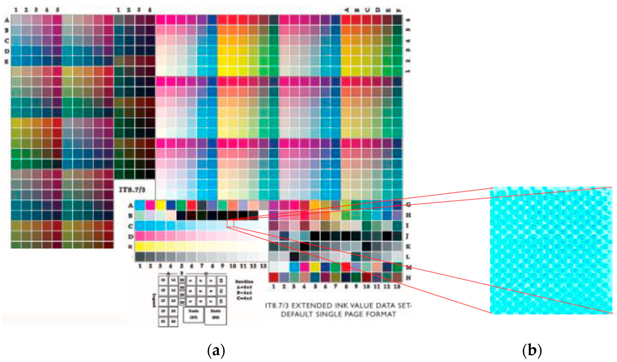
2. Technical Information
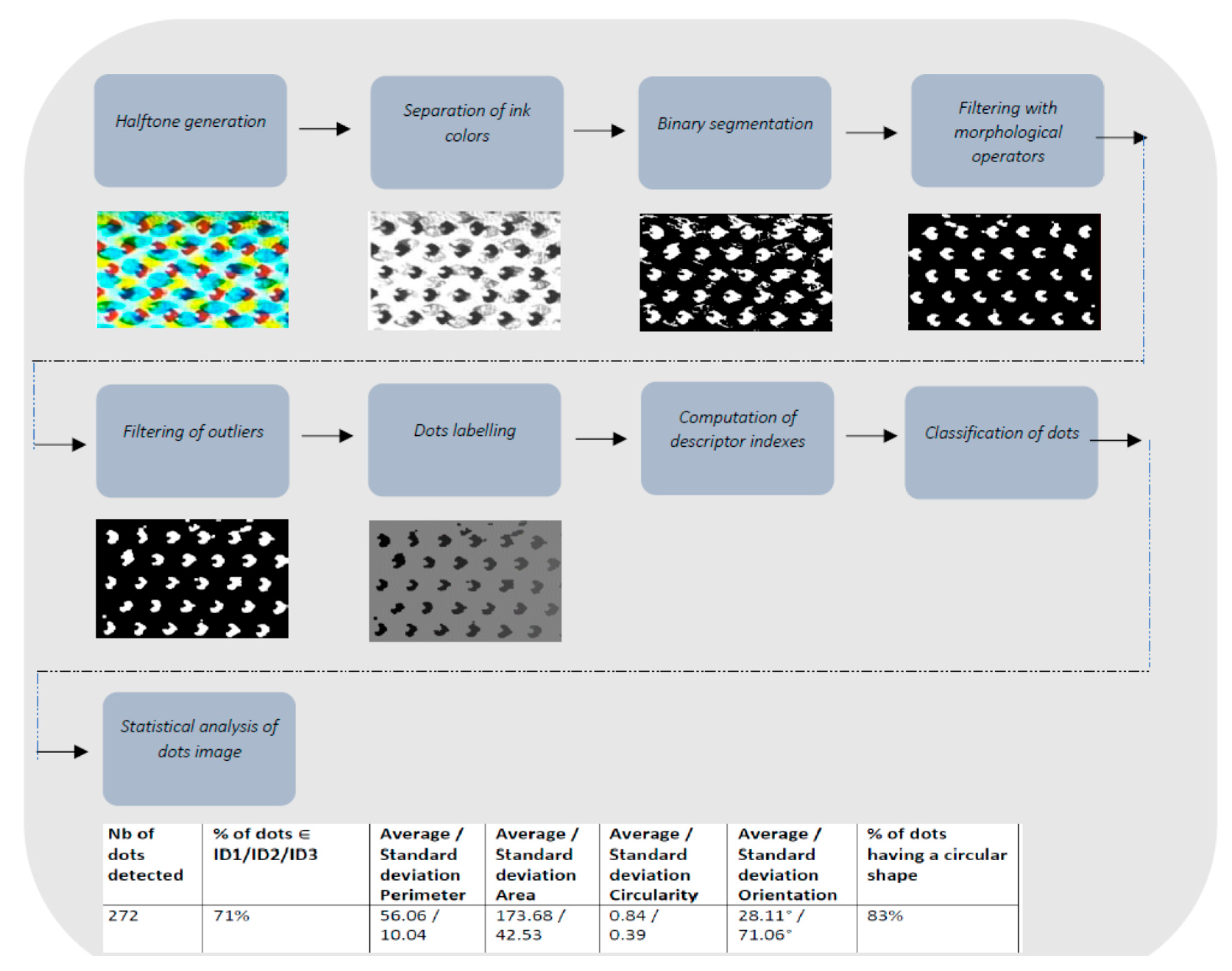
3. Measurement, Modelling and Analysis at the Microscale of Printed Dots
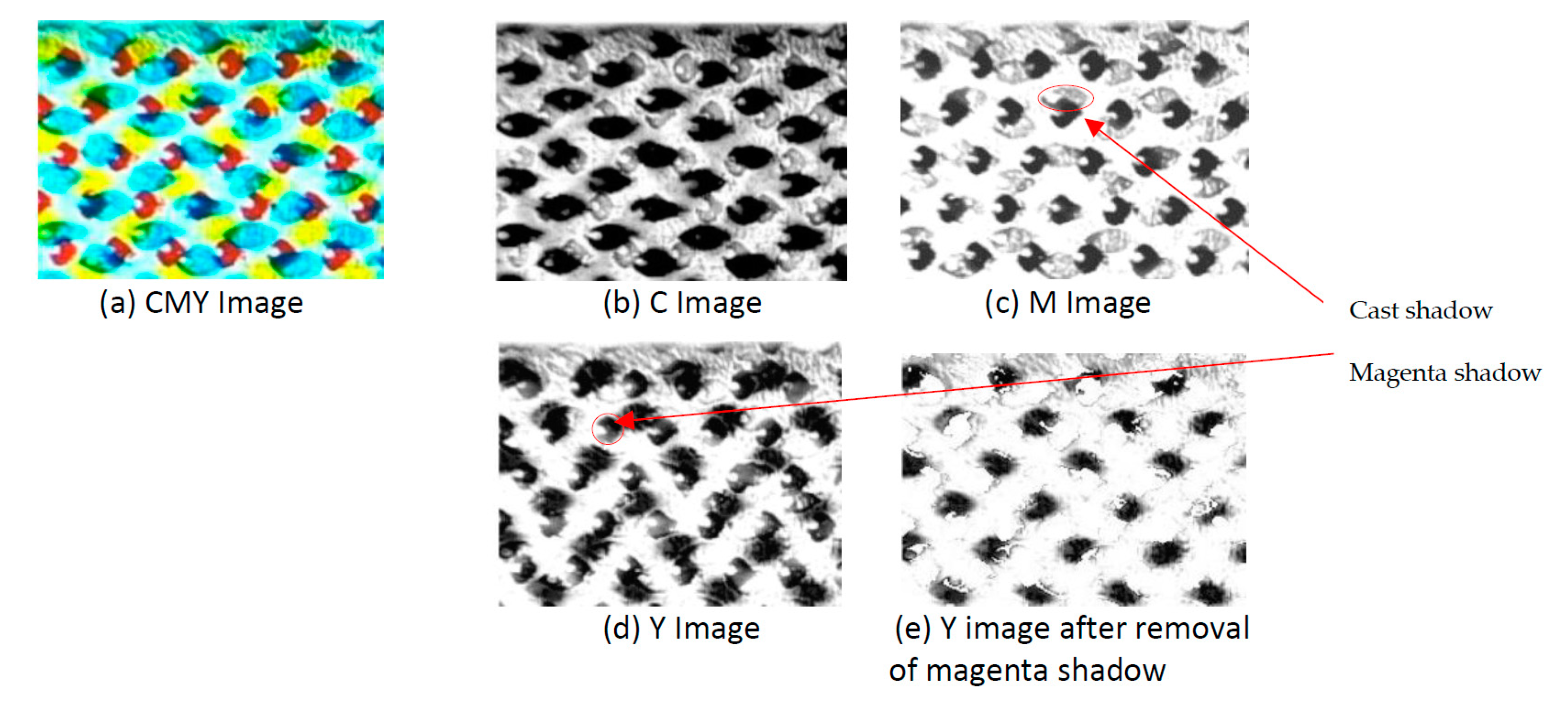
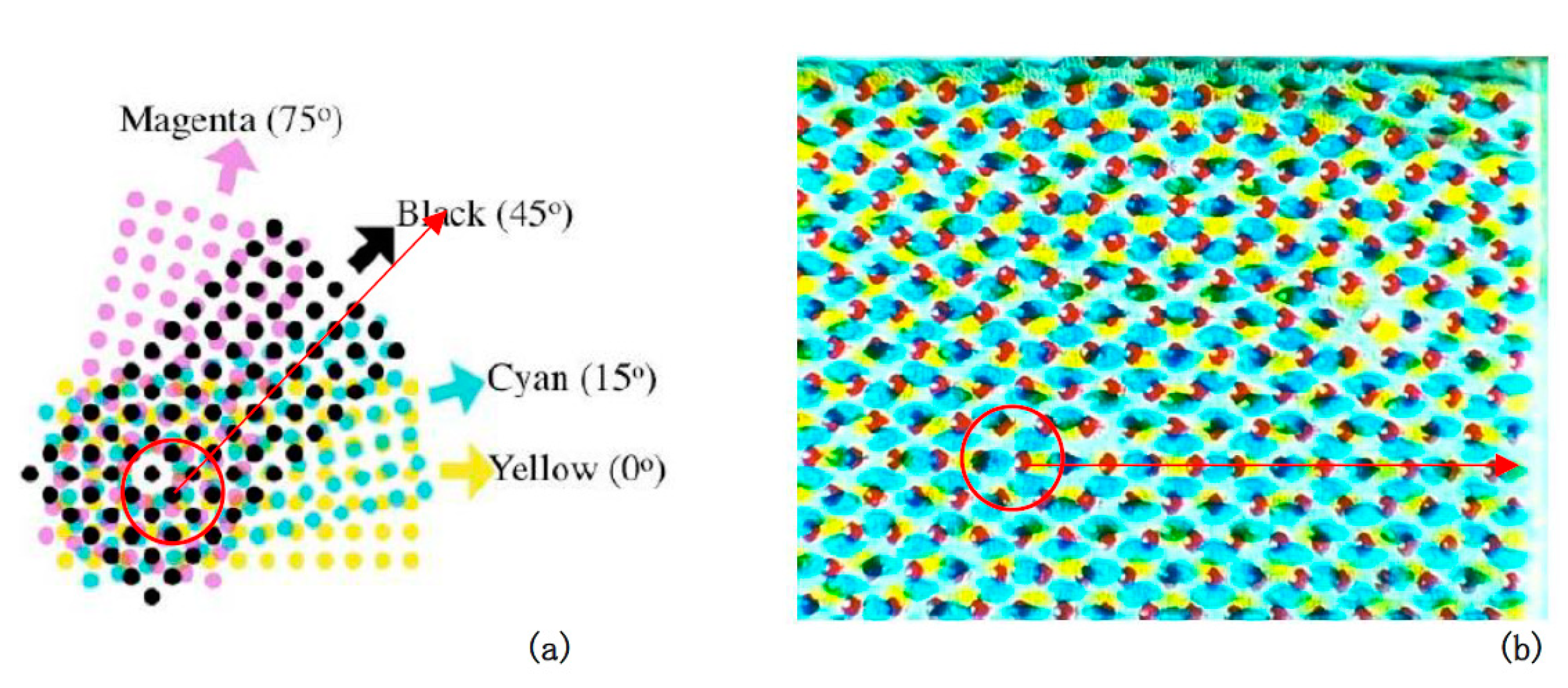
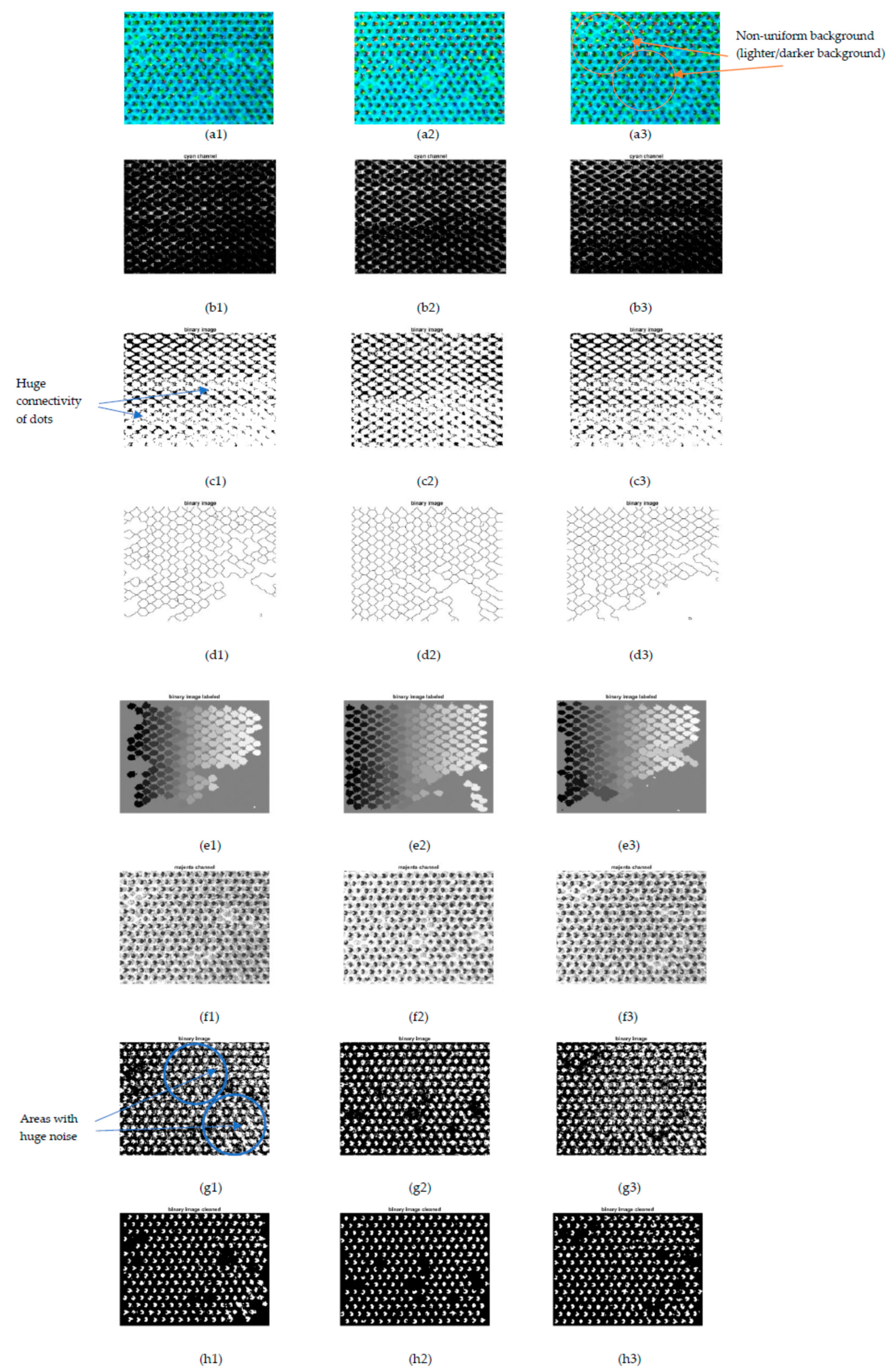
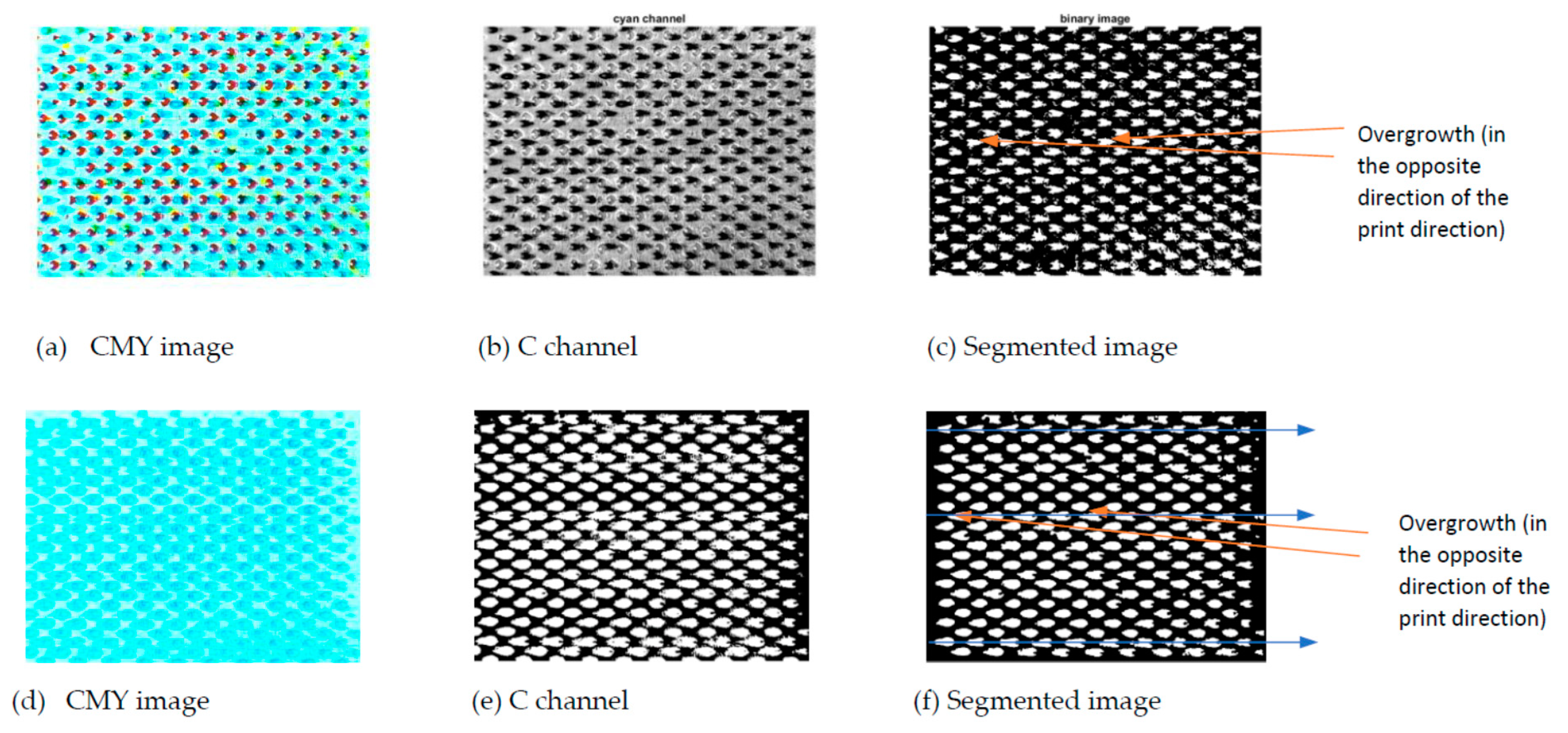
3.1. Separation of Ink Colors (Step 1)
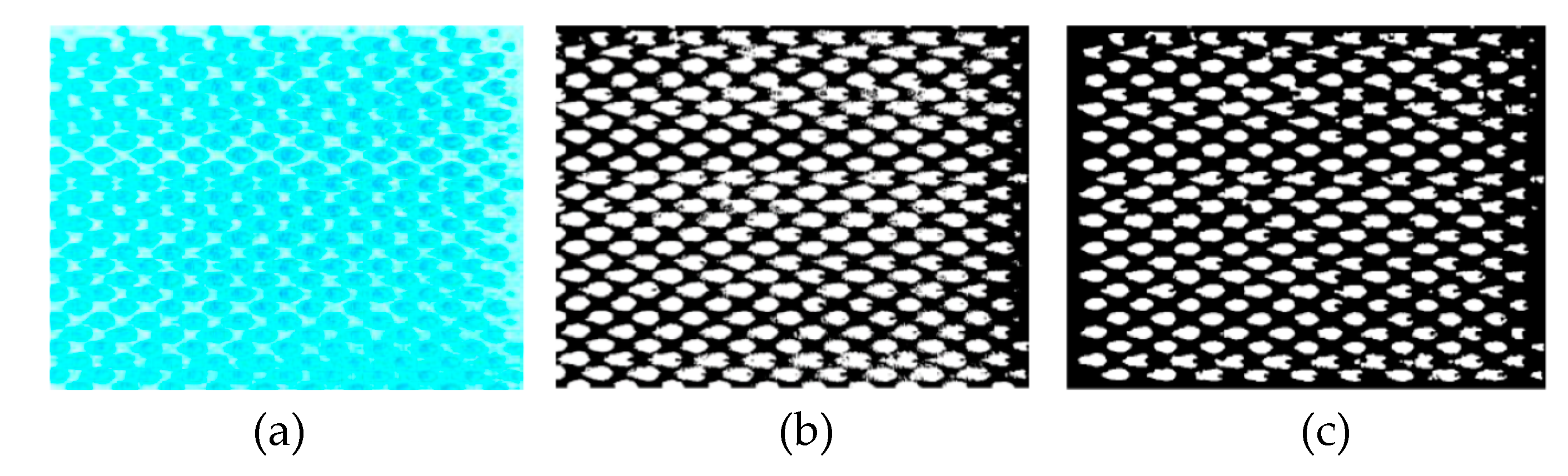
3.2. Binarization of Color Images (Step 2)
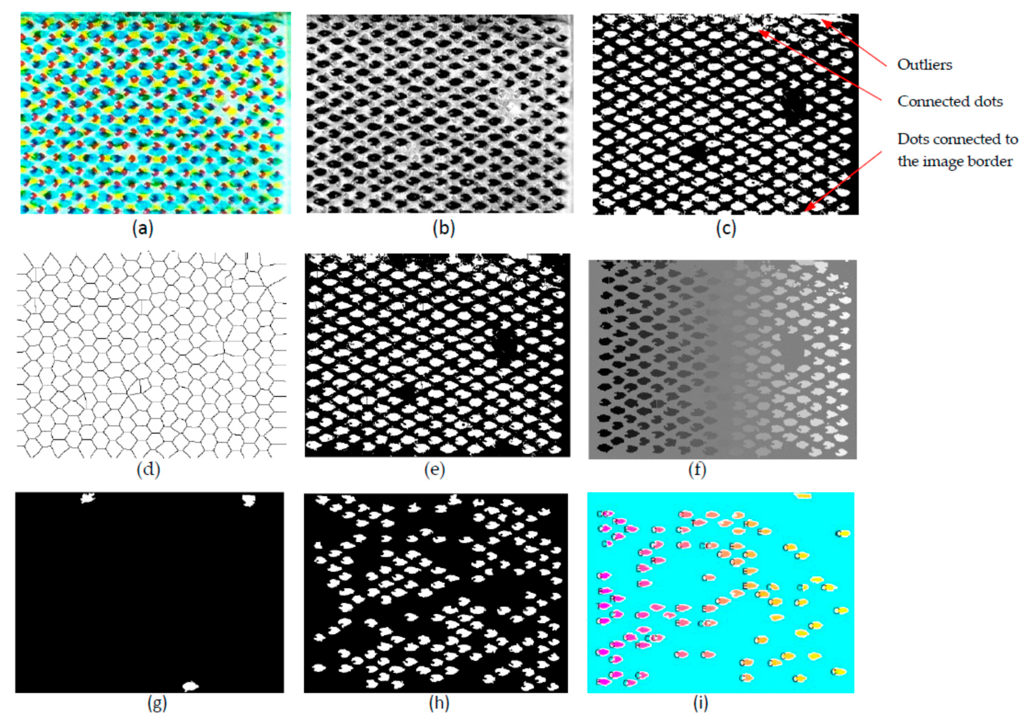
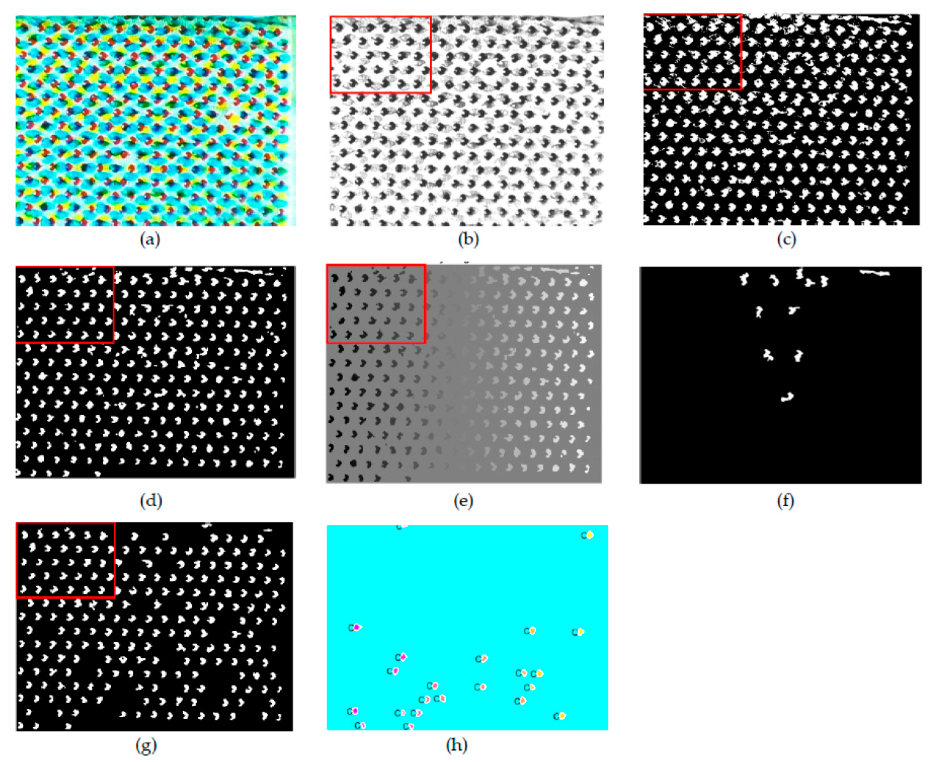
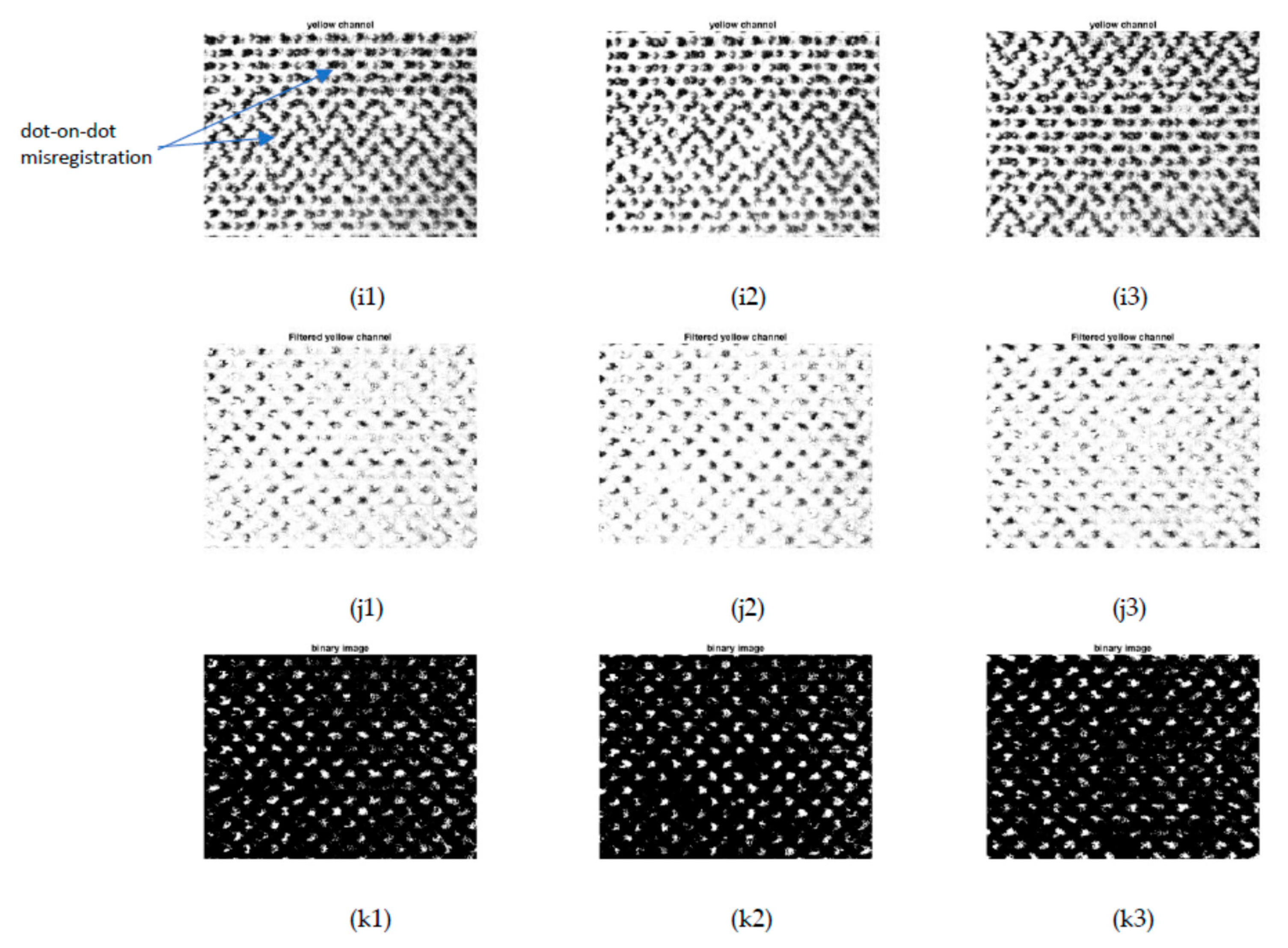
3.3. Filtering of Color Channels (Step 3)
- A removal of dots connected to the image border.
- An erosion with a disk-shaped structuring element of one-pixel radius. This erosion removes isolated pixels (punctual noise) and reduces the border effects due to the physical dot gain on the size of the dots (see Figure 6).
- An opening (erosion followed by a dilation) with a disk-shaped structuring element of one-pixel radius. This opening removes noise and removes small objects from the foreground.
- A removal of small holes in foreground areas with a disk-shaped structuring element of radius 1.
- A watershed transform based on the Euclidean distance. This transform segments contiguous areas into distinct objects, it enables the better separation of connected dots.
3.4. Labelling of Regions of Interest (Step 4)
3.5. Filtering of Outliers (Step 5)
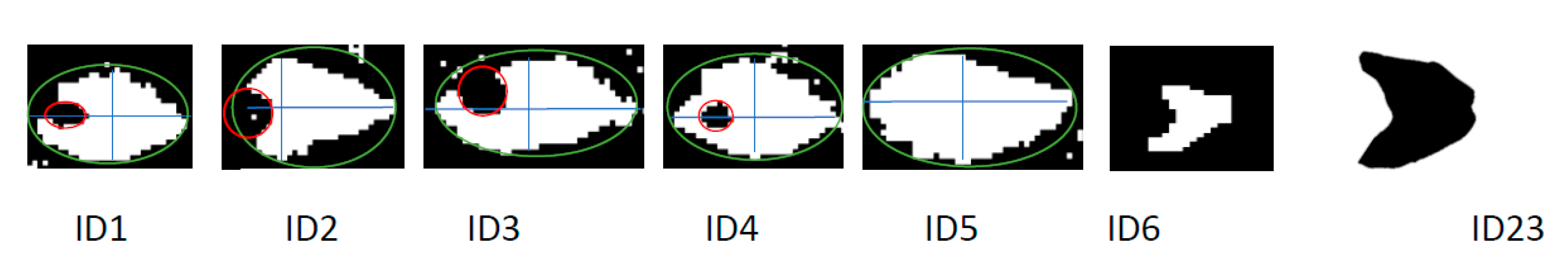
3.6. Computation of Dot Descriptors (Step 6)
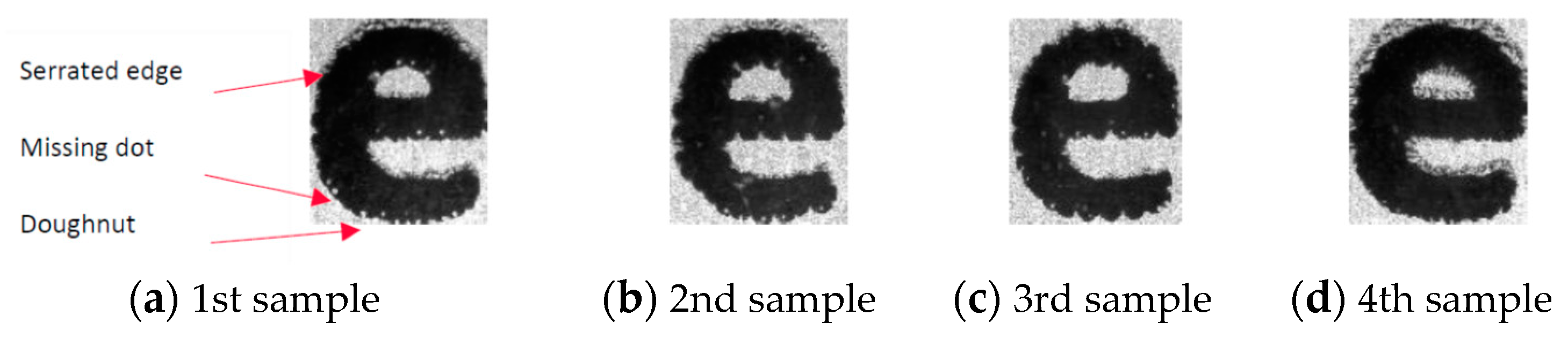
- ID1 narrow doughnut (with a hole inside the convex hull of the dot) with a symmetric shape;
- ID2 concave shape (with a large hole) with a symmetrical shape;
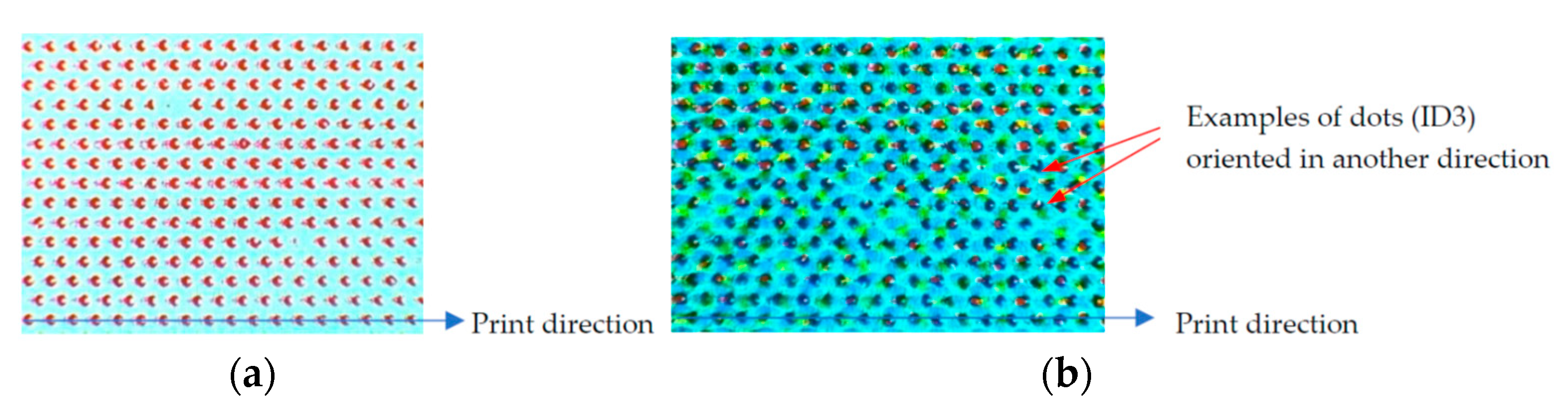
- ID3 concave shape (with a hole inside the convex hull of the dot) with an asymmetric shape;
- ID4 elliptic/circular shape with a hole inside the dot;
- ID5 elliptic/circular shape;
- ID6 random shape;
- Centroid (X, Y coordinates in µm);
- A Area of the dot surface in µm2;
- Ah Area of the hole in the dot in µm2;
- Ac Area of the convex hull of the dot in µm2;
- Ae Area of the elliptic shape bounding the dot in µm2;
- Solidity = A/Ac;
- Perimeter of the dot surface in µm;
- Pc Perimeter of the convex hull of the dot in µm;
- Pe Perimeter of the elliptic shape bounding the dot in µm;
- Convexity = Pc/P;
- Circularity= sqrt(4πA/P2);
- Roundness = sqrt(4πA/Pe2);
- DFmin max Feret diameters in µm;
- Aspect ratio = DFmin/DFmax;
- Orientation = the angle between the x-axis and the major axis of the ellipse that has the same second-moments as the region;
- Major and minor axis;
- Ax1 Area of the dot upper the major axis;
- Ax2 Area of the dot lower the major axis;
- Ay1 Area of the dot at left of the minor axis;
- Ay2 Area of the dot at right of the minor axis;
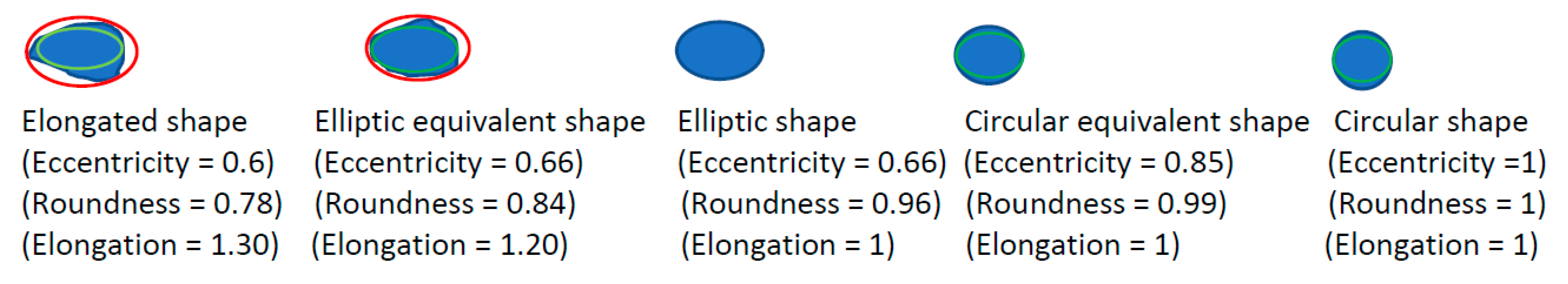
- Eccentricity = length of the minor axis / length of the major axis;
- Elongation along X axis = width of the elliptic bounding box/ width of the highest inscribed ellipse;
- Symmetry relatively to X axis, to Y axis = Ax1/Ax2, = Ay1/Ay2, respectively.
- Concave shapes belonging to category ID1 are defined by an elongation upper than 1.75, a symmetry value Ax1/Ax2 upper than 0.85 and lower than 1.15, and a solidity upper than 0.8.
- Concave shapes belonging to category ID2 are defined by a solidity upper than 0.75 and a symmetry value Ax1/Ax2 upper than 0.85 and lower than 1.15.
- Concave shapes belonging to category ID3 are defined by a solidity upper than 0.75 and a ratio Aij/A upper than 0.15 (assuming that the concavity is in the region Rij).
- Dots belonging to category ID4 have a ratio Ah/A upper than 0.15. Below this value, holes are insignificant.
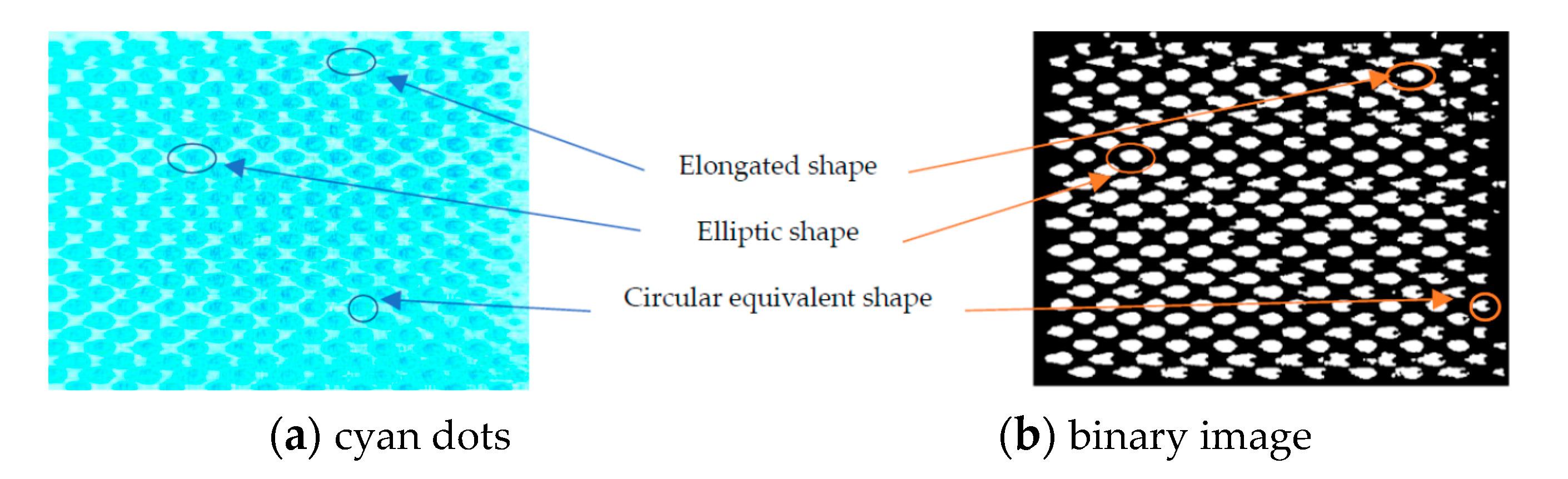
- Circular equivalent dots (see example shown in Figure 11) belonging to category ID5 are defined by a roundness value higher than 0.90 (and an eccentricity upper than 0.85).
- Elliptic equivalent dots (see example shown in Figure 11) belonging to category ID5 are defined by a roundness value between 0.8 and 0.9 (and an eccentricity between 0.6 and 0.85).
- Elongated dots (belonging to category ID6) are defined by an eccentricity lower than 0.6 and a roundness value lower than 0.8 (and an elongation upper than 1.3).
- Any other shape which does not satisfy any of the above rules belongs to category ID6.
3.7. Global Analysis vs. Individual Analysis (Step 7)
4. Experimental Results
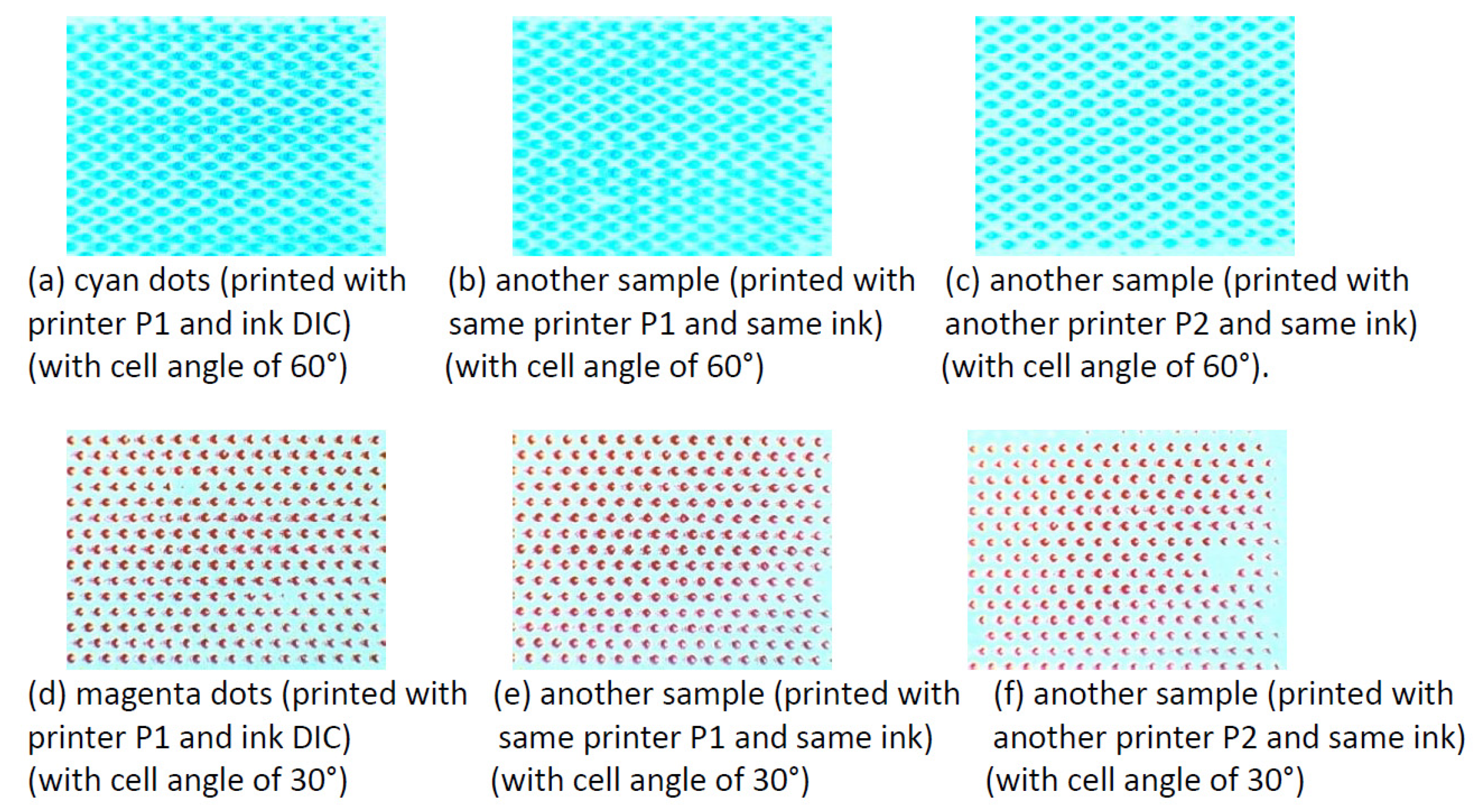
- Samples corresponding to samples number 1, 2, 3, 4, 5 and 6 are very similar in terms of dots shape. As most of the dots are circular, the parameter “orientation” is irrelevant (its standard deviation is very high).
- Samples corresponding to samples number 1, 2, 3, 4, and 5 are very similar (high proportion of doughnuts), meanwhile sample corresponding to sample number 6 is unique (in comparison with these samples) as a significant proportion of its dots have a hole (low proportion of doughnuts).
- The threshold separating “circular equivalent” shapes from “elliptic equivalent” shapes associated with the parameter “circularity” is less robust than the parameter “roundness” which is more relevant to characterize the circularity of non-circle shapes such as the one ∈ ID1/ID2/ID3). As illustration, compare the “circularity” of the sample corresponding to sample number 3 (0.80) with the “circularity” of the sample corresponding to sample number 11 (0.81, see Table 2), these values are similar but visually dots of the first sample are more circular than the second one.
- The shape and size of dots of samples corresponding to samples number 1, 2, 3, 4, 5 and 6 is statistically quite homogeneous (standard deviation values are quite low, for example less than 10 µm for the perimeter).
- Samples corresponding to samples number 11, 12 and 13 (and also to sample number 17, see Table 3) are very similar in terms of dots shape, most of the dots have a “elliptic equivalent” shape oriented in the direction of the print (see Figure 14), which is coherent with the values computed for the parameter “orientation”.
- The proportion of doughnuts is lower than for samples corresponding to samples number 1, 2, 3, 4, 5 and 6 (only 34% for samples number 11 and 12, and less than 8% for samples number 13 and 17). These doughnuts are less visible to the naked eye but are noticeable at microscopic scale. As there are less doughnuts in these samples the “circularity” parameter is more accurate (in the range between 0.81–0.86), which is coherent with an “elliptic equivalent” shape. On the other hand, the standard deviation of “circularity” values is higher (in the range 0.35–0.48), as the dot patterns are more heterogeneous. This is due to a higher standard deviation of the “perimeter” and of the “area” of the dots.
4.1. Prints vs. Reprints
5. Discussion
6. Conclusions
Author Contributions
Funding
Data Availability Statement
Acknowledgments
Conflicts of Interest
References
- Namedanian, M. Characterization of Halftone Prints Based on Microscale Image Analysis; Linköping University Electronic Press: Norrkoping, Sweden, 2013. [Google Scholar]
- Hamblyn, A. Effect of Plate Characteristics on Ink Transfer in Flexographic Printing. Ph.D. Thesis, Swansea University, Swansea, UK, 2015. Available online: http://cronfa.swan.ac.uk/Record/cronfa42827 (accessed on 16 July 2021).
- Nguyen, Q.; Mai, A.; Chagas, L.; Reverdy-Bruas, N. Microscopic Printing Analysis and Application for Classification of Source Printer. Comput. Secur. 2021, 108, 102320. [Google Scholar] [CrossRef]
- Otsu, N. A threshold selection method from gray-level histograms, IEEE Trans. Sys. Man. Cyber. 1979, 9, 62–66. [Google Scholar] [CrossRef] [Green Version]
- Vallat-Evrard, L. Measurement, Analysis and Modelling at the Microscale of Printed Dots to Improve the Printed Anti-Counterfeiting Solutions. Doctoral Dissertation, Chemical and Process Engineering Université Grenoble-Alpes, Grenoble, France, 2019. [Google Scholar]
- Olson, E. Particle Shape Factors and Their Use in Image Analysis–Part 1: Theory. J. GXP Compliance 2013, 15, 85. [Google Scholar]
- Nguyen, Q.T.; Delignon, Y.; Septier, F.; Phan-Ho, A.T. Probabilistic modelling of printed dots at the microscopic scale. Signal Process. Image Commun. 2018, 62, 129–138. [Google Scholar] [CrossRef]
- Tkachenko, I.; Trémeau, A.; Fournel, T. Authentication of Medicine Blister Foils: Characterization of the Rotogravure Printing Process. In Proceedings of the 14th International Joint Conference on Computer Vision, Imaging and Computer Graphics Theory and Applications (VISIGRAPP 2019), Prague, Czech Republic, 25–27 February 2019; pp. 577–583. [Google Scholar] [CrossRef]
- Mathes, H. Flexo troubleshooting. Most common flexo printing issues, Part 3. Flexo Grav. Int. 2011, 4, 22–23. [Google Scholar]
- Sosa, R. Effects of Temperature Control on Gravure Packaging Inks. Master’s Thesis, Western Michigan University, Kalamazoo, Michigan, 1999. Available online: https://scholarworks.wmich.edu/masters_theses/4935 (accessed on 15 July 2021).
- Kader, M.E.A. The Impact of Ink Viscosity on the Enhancement of Rotogravure Optical Print Quality. Int. Des. J. 2017, 7, 103–107. [Google Scholar]
- Joshi, S.; Saxena, S.; Khanna, N. Source Printer Identification from Document Images Acquired using Smartphone. arXiv 2020, 2003, 12602. [Google Scholar]
- Oliver, J.; Chen, J. Use of Signature Analysis to Discriminate Digital Printing Technologies. In Proceedings of the IS&T’s NIP18, International Conference on Digital Printing Technologies, San Diego, CA, USA, 29 September–4 October 2002; pp. 218–222. [Google Scholar]
- Sun, S.; Cao, Z.; Zhu, H.; Zhao, J. A Survey of Optimization Methods from a Machine Learning Perspective. IEEE Trans. Cybern. 2020, 50, 3668–3681. [Google Scholar] [CrossRef] [PubMed] [Green Version]
- Ying, X. An Overview of Overfitting and its Solutions. J. Phys. Conf. Ser. 2019, 1168, 022022. [Google Scholar] [CrossRef]


| N° | Features | Nb of Dots Detected | % of Dots ∈ ID1/ID2/ID3 | Avg ± Std Perimeter | Avg ± Std Area | Avg ± Std Circularity | Avg ± Std Orientation | % of Circular Dots | |
| Reprint Image | |||||||||
| (a) | |||||||||
| 1 |  | 258 | 96% | 49.52 ± 5.92 | 121.79 ± 18.68 | 0.79 ± 0.26 | −23.04° ± 74.94° | 99% | |
| 2 |  | 261 | 96% | 51.6 ± 7.69 | 120.96 ± 23.91 | 0.76 ± 0.30 | 12.40° ± 79.12° | 99% | |
| 3 |  | 237 | 84% (10% ∈ ID6) | 42.05 ± 8.75 | 90.34 ± 25.78 | 0.80 ± 0.37 | −24.17° ± 74.18° | 90% | |
| 4 |  | 242 | 95% | 54.55 ± 7.76 | 135.68 ± 25.68 | 0.76 ± 0.31 | −6.32° ± 80.11 | 96% | |
| 5 |  | 241 | 94% | 54.98 ± 5.19 | 143.34 ± 19.19 | 0.77 ± 0.24 | 40.56° ± 57.43° | 94% | |
| 6 |  | 251 | 3% (40% ∈ ID4) | 62.48 ± 6.51 | 247.12 ± 40.79 | 0.89 ± 0.39 | 22.13° ± 46.09° | 94% (49% ∈ ID5) | |
| N° | Features | Nb of Dots Detected | % of Dots ∈ ID1/ID2/ID3 | Avg ± Std Perimeter | Avg ± Std Area | Avg ± Std Circularity | Avg ± Std Orientation | % of Circular Dots | |
| Reprint Image | |||||||||
| (b) | |||||||||
| 7 |  | 272 | 71% | 56.06 ± 10.04 | 173.68 ± 42.53 | 0.84 ± 0.39 | 28.11° ± 71.06° | 83% | |
| 8 | 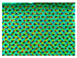 | 278 | 76% | 55.20 ± 9.35 | 161.01± 36.29 | 0.82 ± 0.37 | 35.49° ± 61.78 | 82% | |
| 9 | 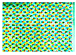 | 287 | 66% | 49.84 ± 10.79 | 137.19 ± 37.66 | 0.84 ± 0.42 | 31.8° ± 63.0° | 72% | |
| 10 |  | 258 | 32% (42 % ∈ ID4) | 63.95 ± 7.68 | 199.48 ± 33.24 | 0.79 ± 0.31 | 10.7° ± 75.43° | 75% | |
| N° | Features | Nb of Dots Detected | % of Dots ∈ID1/ID2/ID3 | Avg ± Std Perimeter | Avg ± Std Area | Avg ± Std Circularity | Avg ± Std Orientation | % of Elliptic Dots | |
| Print Image | |||||||||
| (a) | |||||||||
| 11 | 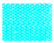 | 267 | 34% | 86.51 ± 20.40 | 373.45 ± 105.36 | 0.81 ± 0.42 | −1.20 ° ± 7.82° | 18% (37% have a circular shape) (55% ∈ ID5) | |
| 12 | 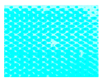 | 265 | 34% (4% ∈ ID6) (6% of connected dots not analyzed) | 94.78 ± 27.20 | 487.83 ± 170.23 | 0.84 ± 0.48 | −2.0° ± 18.80° | 35% (10% have a circular shape) (45% ∈ ID5) | |
| 13 |  | 249 | 8% (6% of connected dots not analyzed) | 93.50 ± 22.67 | 481.32 ± 153.78 | 0.83 ± 0.39 | 1.81° ± 5.56° | 24% (31% have a circular shape) (86% ∈ ID5, among them 31% are nor circular nor elliptic) | |
| N° | Features | Nb of Dots Detected | % of Dots ∈ID1/ID2/ID3 | Avg ± Std Perimeter | Avg ± Std Area | Avg ± Std Circularity | Avg ± Std Orientation | % of Elliptic Dots | |
| Reprint Image | |||||||||
| (b) | |||||||||
| 14 |  | 246 | 40% (35% ∈ ID6) | 63.80 ± 9.81 | 203.20 ± 38.51 | 0.80 ± 0.31 | 5.44° ± 13.90° | 21% (25 % ∈ ID5) | |
| 15 | 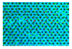 | 250 | 4% (15% ∈ ID6) (28% of connected dots not analyzed) | 86.79 ± 67.14 | 483.47 ± 205.37 | 0.92 ± 0.53 | 3.63° ± 19.2° | 31% (17% have a circular shape) (53 % ∈ ID5) | |
| 16 |  | 250 | 8% (23% ∈ ID6) (22% of connected dots not analyzed) | 87.84 ± 65.70 | 464.39 ± 232.34 | 0.93 ± 0.56 | 4.23° ± 21.2° | 28% (15% have a circular shape) (47 % ∈ ID5) | |
| N° | Features | Nb of Dots Detected | % of Dots ∈ID1/ID2/ID3 | Avg ± Std Perimeter | Avg ± Std Area | Avg ± Std Circularity | Avg ± Std Orientation | % of Elliptic Dots | |
|---|---|---|---|---|---|---|---|---|---|
| Print Image | |||||||||
| 17 | 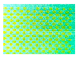 | 156 | 6% (7% ∈ ID6) | 91.04 ± 13.58 | 484.19 ± 91.77 | 0.86 ± 0.35 | −1.01° ± 11.65° | 75% (80% ∈ ID5) | |
| 18 |  | 199 | 30% (30% ∈ ID6) | 56.08 ± 23.90 | 188.63 ± 121.81 | 0.87 ± 0.52 | 5.96° ± 44.76° | 32% (38% ∈ ID5) | |
Publisher’s Note: MDPI stays neutral with regard to jurisdictional claims in published maps and institutional affiliations. |
© 2021 by the authors. Licensee MDPI, Basel, Switzerland. This article is an open access article distributed under the terms and conditions of the Creative Commons Attribution (CC BY) license (https://creativecommons.org/licenses/by/4.0/).
Share and Cite
Das, I.; Bandyopadhyay, S.; Trémeau, A. Characterization of Prints Based on Microscale Image Analysis of Dot Patterns. Appl. Sci. 2021, 11, 6634. https://doi.org/10.3390/app11146634
Das I, Bandyopadhyay S, Trémeau A. Characterization of Prints Based on Microscale Image Analysis of Dot Patterns. Applied Sciences. 2021; 11(14):6634. https://doi.org/10.3390/app11146634
Chicago/Turabian StyleDas, Indrama, Swati Bandyopadhyay, and Alain Trémeau. 2021. "Characterization of Prints Based on Microscale Image Analysis of Dot Patterns" Applied Sciences 11, no. 14: 6634. https://doi.org/10.3390/app11146634
APA StyleDas, I., Bandyopadhyay, S., & Trémeau, A. (2021). Characterization of Prints Based on Microscale Image Analysis of Dot Patterns. Applied Sciences, 11(14), 6634. https://doi.org/10.3390/app11146634