Empowering Advanced Parametric Modes Clustering from Topological Data Analysis

Featured Application

This paper aims at proposing the use of a topological metrics based on the persistent homology, enabling efficient surfaces classification, and ordering the elastodynamics eigenmodes to construct parametric reduced bases.

Abstract

Modal analysis is widely used for addressing NVH—Noise, Vibration, and Hardness—in automotive engineering. The so-called principal modes constitute an orthogonal basis, obtained from the eigenvectors related to the dynamical problem. When this basis is used for expressing the displacement field of a dynamical problem, the model equations become uncoupled. Moreover, a reduced basis can be defined according to the eigenvalues magnitude, leading to an uncoupled reduced model, especially appealing when solving large dynamical systems. However, engineering looks for optimal designs and therefore it focuses on parametric designs needing the efficient solution of parametric dynamical models. Solving parametrized eigenproblems remains a tricky issue, and, therefore, nonintrusive approaches are privileged. In that framework, a reduced basis consisting of the most significant eigenmodes is retained for each choice of the model parameters under consideration. Then, one is tempted to create a parametric reduced basis, by simply expressing the reduced basis parametrically by using an appropriate regression technique. However, an issue remains that limits the direct application of the just referred approach, the one related to the basis ordering. In order to order the modes before interpolating them, different techniques were proposed in the past, being the Modal Assurance Criterion—MAC—one of the most widely used. In the present paper, we proposed an alternative technique that, instead of operating at the eigenmodes level, classify the modes with respect to the deformed structure shapes that the eigenmodes induce, by invoking the so-called Topological Data Analysis—TDA—that ensures the invariance properties that topology ensure.

1. Introduction

Linear structural solid dynamics [1] expressed in the time domain results in the linear system of second order ordinary differential equations

$$\mathbf{M}\frac{d^2\mathbf{U}\left(t\right)}{d{t}^2}+\mathbf{C}\frac{d\mathbf{U}\left(t\right)}{dt}+\mathbf{K}\mathbf{U}\left(t\right)=\mathbf{F}\left(t\right),$$

(1)

with the mass, damping, and stiffness matrices given by $\mathbf{M}$, $\mathbf{C}$, and $\mathbf{K}$ respectively, $\mathbf{U}$ the vector that contains the nodal displacements, and $\mathbf{F}$ the applied nodal forces. Its time integration can be performed by using any well experienced state of the art discretization technique, as [2] or [3].

In what follows, we will omit the damping term that results from the fact of assuming a proportional damping that expresses it as a combination of the mass and stiffness contributions.

To enhance the integration efficiency, mass lumping is usually considered, leading to a mass diagonal matrix. Model analysis looks also for enhancing the solution efficiency by decoupling the motion equation. For that purpose, the last extracts the basis $\{{\mathbf{\varphi }}_1,{\mathbf{\varphi }}_2,\dots ,{\mathbf{\varphi }}_{\mathtt{N}}\}$ (N being the problem size, i.e., the number of degrees of freedom) by solving the eigenproblem

$$\left(-{\omega }^2\mathbf{M}+\mathbf{K}\right)\mathbf{\varphi }=\mathbf{0},$$

(2)

associated with the dynamical problem expressed in the Fourier space,

$$\left(-{\omega }^2\mathbf{M}+\mathbf{K}\right)\mathcal{U}=\mathcal{F},$$

(3)

where $\mathcal{U}$ and $\mathcal{F}$ refer to the Fourier transform of the nodal displacement $\mathbf{U}$ and forces $\mathbf{F}$.

The eigenmodes ${\mathbf{\varphi }}_i$, $i=1,\dots ,N$ define an orthogonal basis, normalized with respect to the mass matrix, i.e.,

$${\mathbf{\varphi }}_i^T\mathbf{M}{\mathbf{\varphi }}_j={\delta }_{ij},$$

(4)

with $\delta$ the Kroenecker delta, and

$${\mathbf{\varphi }}_i^T\mathbf{K}{\mathbf{\varphi }}_j={\kappa }_i{\delta }_{ij}.$$

(5)

With $\mathbf{P}$ the matrix composed by the eigenmodes, i.e., $\mathbf{P}=({\mathbf{\varphi }}_1,\dots ,{\mathbf{\varphi }}_N)$, the matrix form of the previous expressions reads ${\mathbf{P}}^T\mathbf{M}\mathbf{P}=\mathbf{I}$ and ${\mathbf{P}}^T\mathbf{K}\mathbf{P}=\mathbb{K}$, with $\mathbf{I}$ the identity matrix and $\mathbb{K}$ the diagonal matrix with entries ${\mathbb{K}}_{ii}={\kappa }_i$.

In the modal basis $\mathbf{U}=\mathbf{P}\mathbf{\phi }$, the dynamical problem reads

$$\mathbf{I}\frac{d^2\mathbf{\phi }\left(t\right)}{d{t}^2}+\mathbb{K}\mathbf{\phi }\left(t\right)={\mathbf{P}}^T\mathbf{F}\left(t\right),$$

(6)

which constitutes a system of $\mathtt{N}$ uncoupled second order ordinary differential equations.

The main limitation of modal analysis is the lack of validity of such basis in the case of parametric models. In the case of parametrized dynamical systems, with the model parameters grouped in vector $\mathbf{\mu }$, the model matrices will depend on those parameters, i.e., $\mathbf{M}\left(\mathbf{\mu }\right)$ and $\mathbf{K}\left(\mathbf{\mu }\right)$. The solution of parametric eigenproblems remains a tricky issue.

When one is not really interested in the transient regime, but much more in the forced regime, harmonic analysis represents a valuable route as considered in our former works where the so-called Proper Generalized Decomposition—PGD—enabled considering the frequency as a model extra-parameter as well as addressing general (non-proportional) damping and nonlinear dynamics, under the stringent real-time constraint, with even the inclusion of model parameters as extra-coordinates [4,5,6].

However, certain applications need accurate transient responses, and in that case the formulation and solution of the dynamical problem in the time domain is retained. Three routes are usually considered:

• The previously referred mass lumping that transforms the so-called consistent mass matrix into its diagonal counterpart, facilitating an explicit integration;
• In the context of model order reduction—MOR—, in [7], authors proposed a Proper Orthogonal Decomposition—POD—based reduced order modeling operating in the time domain. Ladeveze and coworkers proposed an extension of their radial approximation [8] for addressing mid-frequency dynamics, the so called TVCR (variational theory of complex rays) [9]. In our former works, we considered a PGD formulation for constructing a parametric transfer function [10] that allowed efficient solutions of transient dynamics operating in the time-domain. On the other hand, the separation of variables, at the heart of PGD [11], was extensively employed in the harmonic domain for solving multi-parametric dynamics, and was successfully extended to the nonlinear case, and then combined with modal analysis [4,5,6].
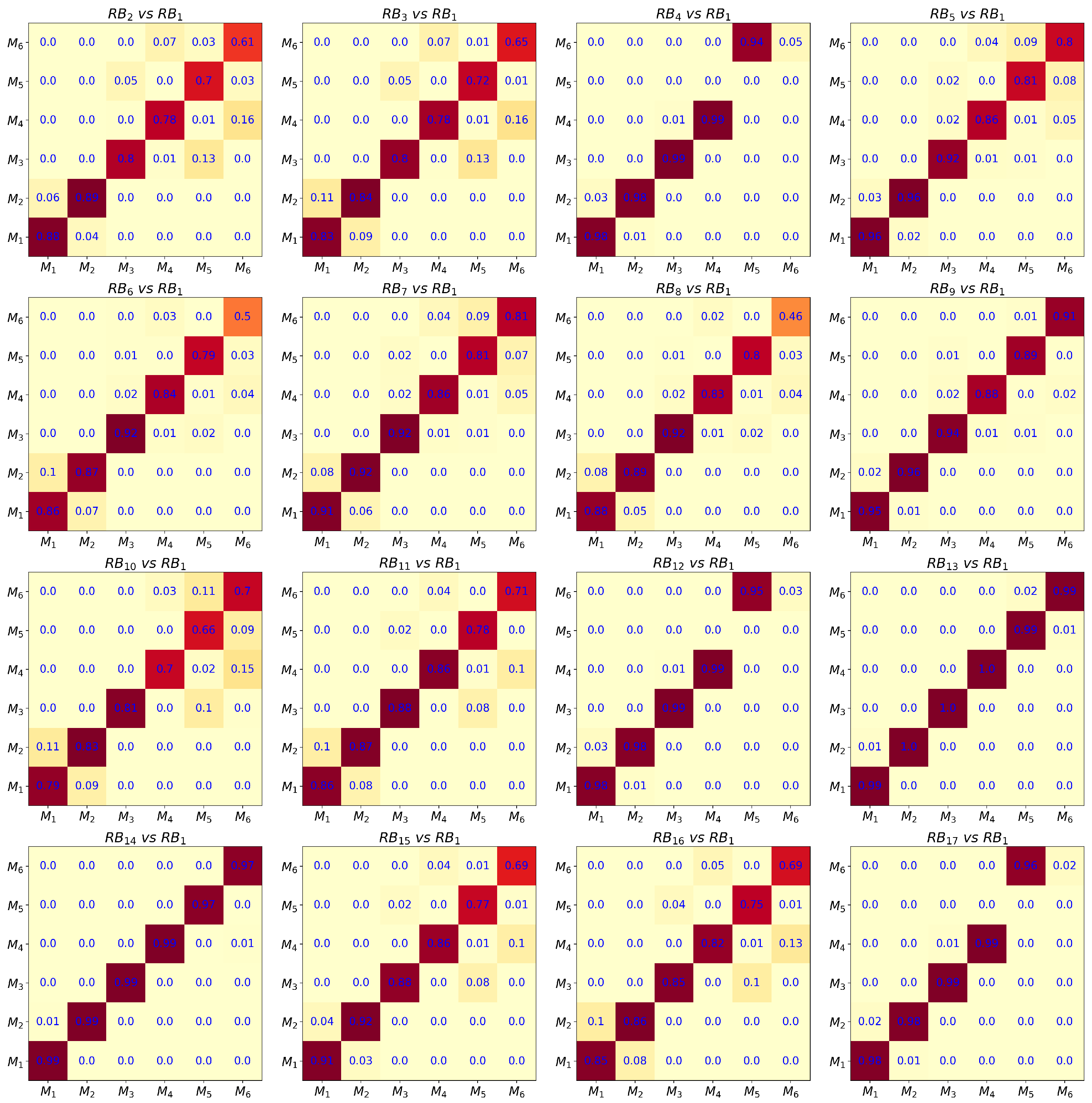
• Modal analysis is one the most widely used techniques for solving dynamical problems. Other than the benefits in the time integration, due to the dynamical system decoupling, the eigenmodes benefit from a physical interpretation, of great interest for the designer or structural analyst. However, when considering parametric models, as is always the case during the design stage, when the material and geometry are not totally defined, the dynamical modes depend on those parameters as previously discussed. Having a surrogate model expressing the parametric evolution of the eigenmodes is of great interest. Constructing those surrogate models is nowadays quite mature, by using usual and advanced nonlinear regressions [12], the last making use of sparsity and appropriate regularizations for operating in high-dimensional settings, while keeping as reduced as possible the number of data (eigenproblem solution), and leading to rich enough (nonlinear) regressions while avoiding overfitting. Here, the trickiest issue is not the regression construction but the fact of ordering the different eigenmodes involved in the modal basis for each parameter choice, in order to create N clusters (or less in the reduced case), and putting in each one a mode of each modal basis, such that modes in each cluster remain close (in certain metrics). The main issue remains the metric to be used to successfully and efficiently accomplishing such clustering. In general, such clustering is performed by operating at the level of the eigenmodes, in the associated vector space, by using, for example, the Modal Assurance Criterion—MAC— [13] that proceed with comparing the modes resulting from each eigenproblem, by using the usual scalar product (modes similar to a given one should remain quite collinear).

The present paper focuses on the techniques based on modal analysis. As just described, usual techniques operate at the eignemodes level, defined in a vector space. When operating in high dimensional parametric spaces, sparsely sampled, the matrices involved in the resulting eigenproblem can vary a lot from one choice of the parameters to another, and consequently the scalar product criterion at the basis of the MAC could fail. On the other hand, the fact of proceeding in a vector space needs to carefully address the expression of the different modes by considering the same frame for all the analyzed mechanical systems.

For alleviating those difficulties, this paper proposes an alternative technique that instead of operating at the eigenmodes level, classifies the modes with respect to the deformed structures shape that the eigenmodes produce, by invoking the so-called Topological Data Analysis—TDA— that benefits from the invariance property of topology. The present paper does not aim at addressing the interpolation between the original and deformed structures that could be addressed by using optimal transport, or the parametrization of the manifold as in the parallel transport [14]. The present work aims only at addressing the deformed structures comparison using an appropriate metric, in particular the one based on the employment of TDA.

After the above short introduction, Section 2 addresses the problem and methodologies employed, Section 3 reports the obtained results, and Section 4 discusses the obtained results emphasizing the added value of the proposed approach.

2. Methods

As just indicated, the present paper aims at addressing the classification of a series of modal basis related to the eigenmodes of a thin structure equipped with a mesh consisting of shell elements, with displacement and rotation degrees of freedom at each node of the mesh.

The thickness of the structural part varies, with its consequent effect on the mass and stiffness matrices (damping is assumed proportional) and consequently on the eigenvalues and eigenvectors, the former defining the number of modes to be retained in the reduced basis. In the present study, the six rigid modes representing the whole structure translation (three modes) and rotation (three modes) will be discarded and among the remaining pairs eigenvalue-eigenvector, the most relevant six eigenvectors (corresponding to the six highest eigenvalues) retained in the reduced basis related to each choice of the model parameter (the thickness).

These six modes related to each structure (related to a thickness value) define a reduced basis that one would like render parametric. However, prior to constructing a regression able to define the reduced basis for each possible choice of the parameter (thickness), one should classify the six eigenmodes of each reduced basis associated with each structure into six clusters.

This task is compulsory to facilitate the interpolation in the parametric space and also to attach a physical sense to those modes. One could imagine that, for a given thickness, the most relevant deformation mode could be related to the extension, whereas, for another choice of the thickness, the most relevant deformation mode could be the bending. In such a case, one prefers to create a cluster grouping similar deformation modes, to evaluate how each of them depends on the parameter from one side, and on the other to facilitate the subsequent construction of the parametric modal reduced basis.

To preform such a clustering, we must employ an appropriate metric to compare those modes. In general, this comparison was traditionally performed by comparing the eigenmodes within the vector space to which they belong. In the present work, as announced previously, we prefer applying the deformation mode to the reference (undeformed) structure, that is, applying the eigenmode at the nodes location in the reference structure for obtaining the deformed structure related to each mode of each structure configuration (thickness) and then clusterizing the resulting deformed structures with respect to their shape.

Thus, we are employing a metric able to compare shapes, more than a metric for comparing the vectors (eigenmodes) that produced those shapes, the last being more intrinsic and inheriting invariance features. Moreover, in the present case study, eigenmodes are heterogeneous in the sense that they involve displacements and rotations, whereas the associated deformed surfaces are purely geometrical. For that purpose, the TDA will be applied.

In the remaining part of the present section, we will describe the available data and its organization, and then all the concepts enabling the use of a metric applying on the shapes, based on the employment of persistent homology, at the heart of the TDA, employed in our former works [15,16].

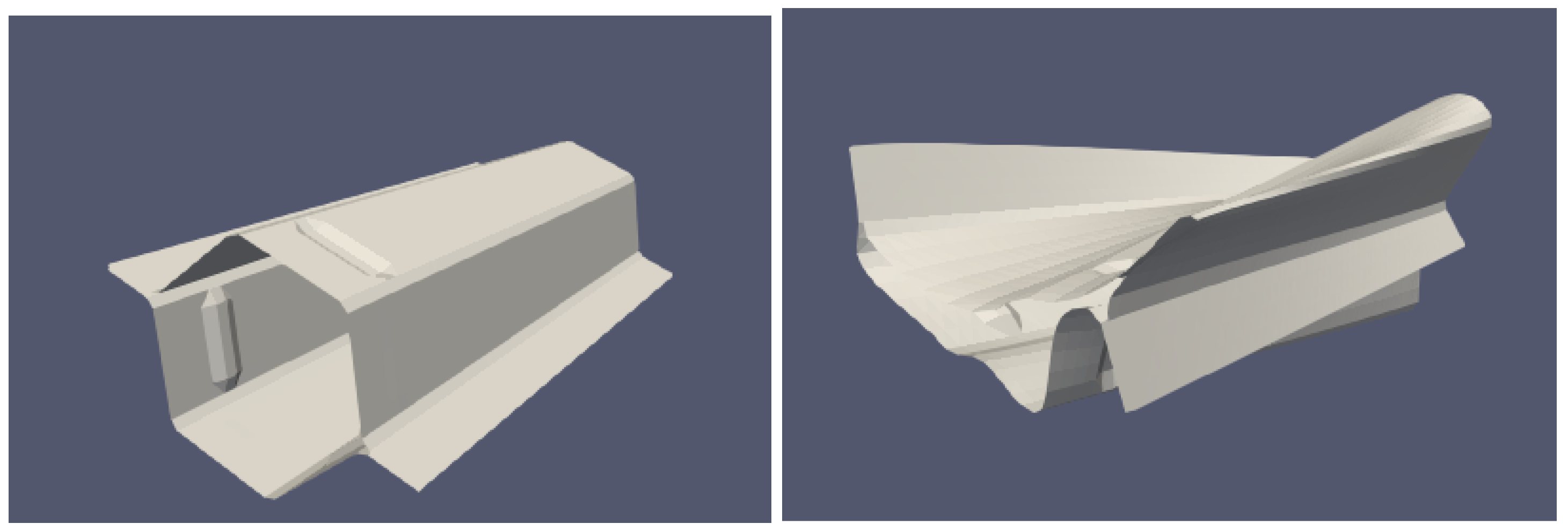
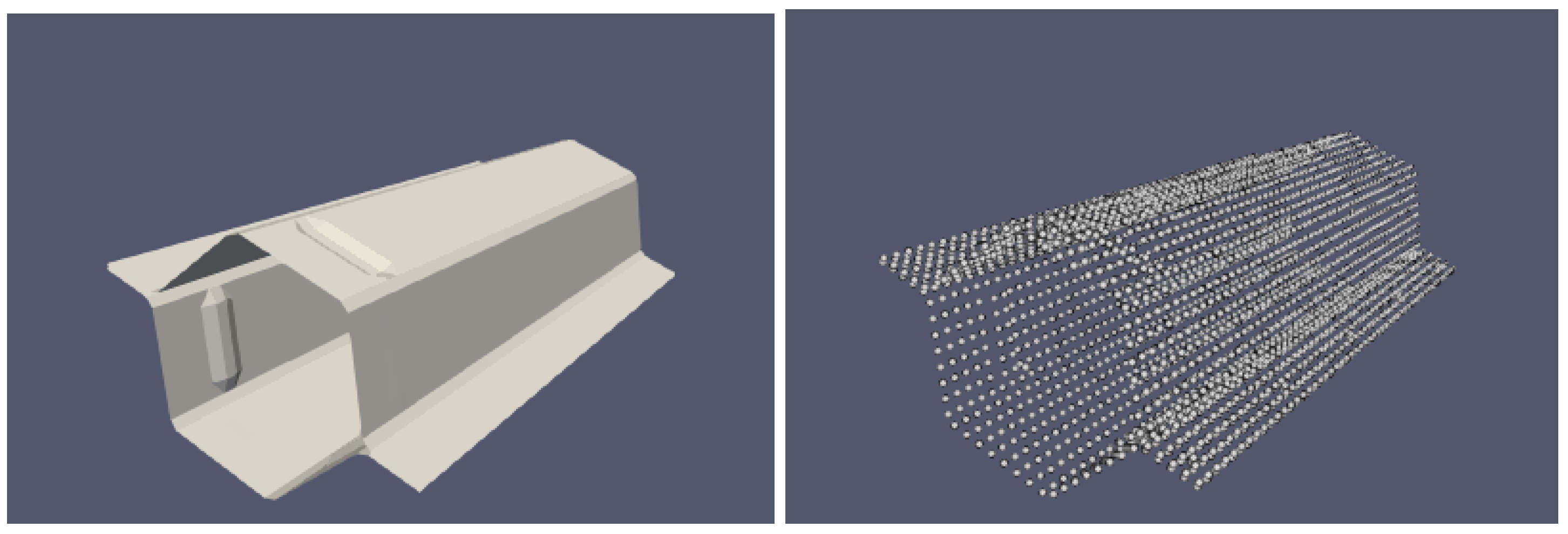
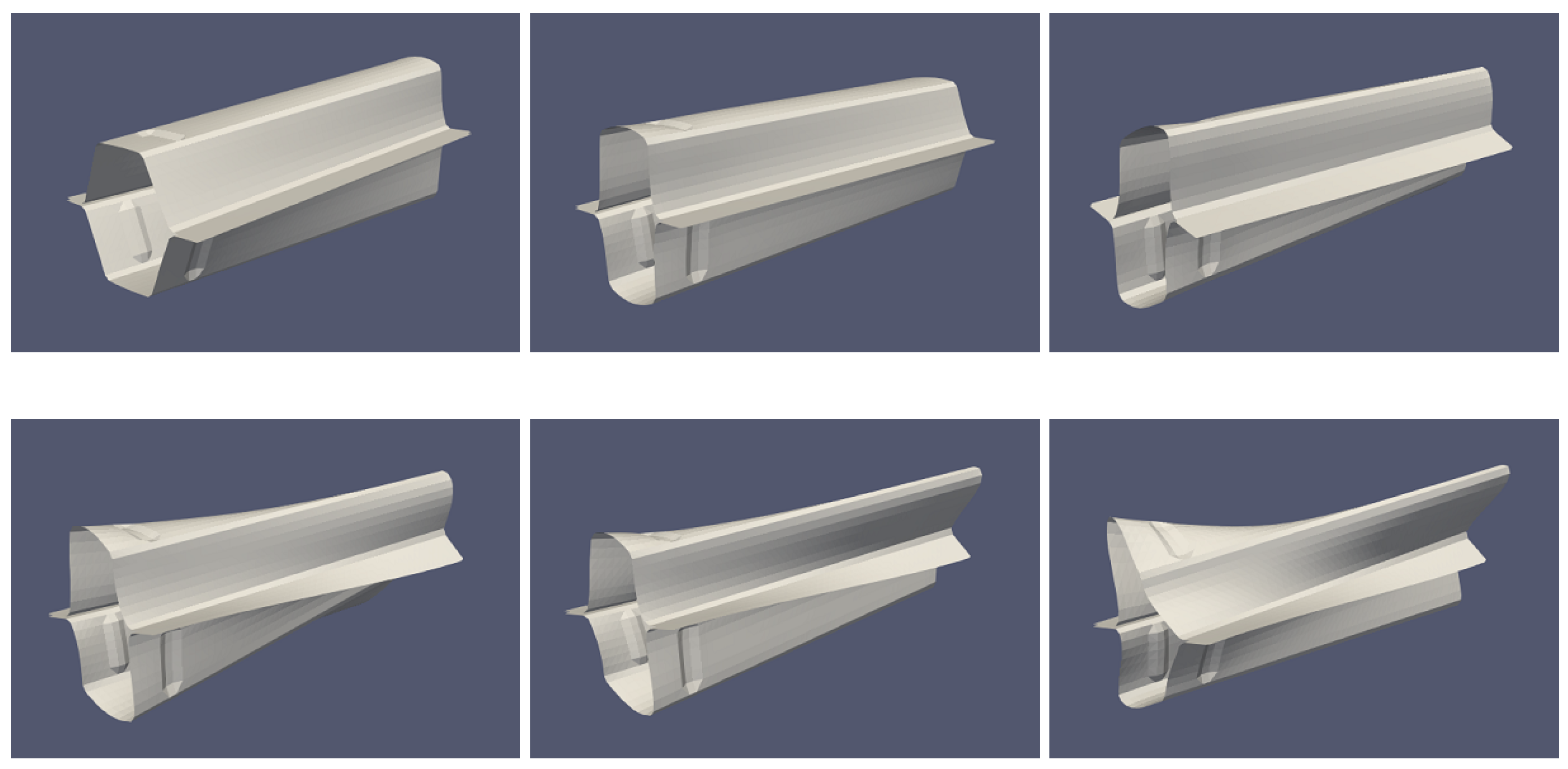
2.1. Data Description

As the different analyzed structures are shells of different thicknesses, from now on, we will describe these structures by their surfaces, each equipped of a node distribution and the associated mesh.

In this study, we consider a collection of $\mathcal{M}=102$ surfaces corresponding to the effect of a given deformation mode on the reference undeformed surface, as Figure 1 shows.

Each surface ${\mathbb{M}}_r$, $r=1,\dots ,\mathcal{M}$ is equipped with a mesh associated with $\mathcal{N}=3636$ nodes, each node described by ${\mathbf{x}}_n\equiv (x_n,y_n,z_n)$, $n=1,\dots ,\mathcal{N}$ and ${\mathbf{x}}_n\in {\mathbb{R}}^3$, all them making use of the same common coordinates frame.

The deformed structures consist of the nodes and elements resulting from the reference one by applying the associated deformation mode. There is neither nodes’ redistribution nor refinement in the deformed surfaces. Figure 2 depicts the reference surface and the nodes distribution on it, from which all the deformed structures with their associated nodal distribution and deformed mesh will result. It is important to note that the undeformed and deformed meshes (elements connectivity) remain unchanged, facilitating the use of the proposed metrics discussed later.

The $\mathcal{M}=102$ surfaces are associated with 17 different structures, each one of them having a different thickness, with the consequent effect on the mass and stiffness matrices, and therefore on the resulting eigenfrequencies and eigenmodes. For each of the 17 structures, the six most significant deformation modes (related to the six highest eigenvalues with the rigid modes excluded) are retained. As mentioned, by applying this $17\times 6$ deformation modes to the original undeformed reference surface, the $\mathcal{M}=102$ deformed surfaces result.

The data are structured as a table, and, within each row, the six deformation modes related to a given structure (with its own thickness) are as follows:

$$\begin{array}{cccccc}{\mathbb{M}}_1& {\mathbb{M}}_2& {\mathbb{M}}_3& {\mathbb{M}}_4& {\mathbb{M}}_5& {\mathbb{M}}_6\\ {\mathbb{M}}_7& {\mathbb{M}}_8& {\mathbb{M}}_9& {\mathbb{M}}_{10}& {\mathbb{M}}_{11}& {\mathbb{M}}_{12}\\ \dots & \dots & \dots & \dots & \dots & \dots \\ {\mathbb{M}}_{97}& {\mathbb{M}}_{98}& {\mathbb{M}}_{99}& {\mathbb{M}}_{100}& {\mathbb{M}}_{101}& {\mathbb{M}}_{102}\end{array}$$

Our main aim in what follows is ordering the elements in the columns, such that each column will represent a similar deformation behavior.

2.2. On the Surface Topology

Consider a data-set $\mathbb{M}$ related to a given deformed surface defined from its $\mathcal{N}$ nodes, all of them in ${\mathbb{R}}^3$. We are interested in extracting the geometric features of $\mathbb{M}$ and how they are distributed across the different spatial scales.

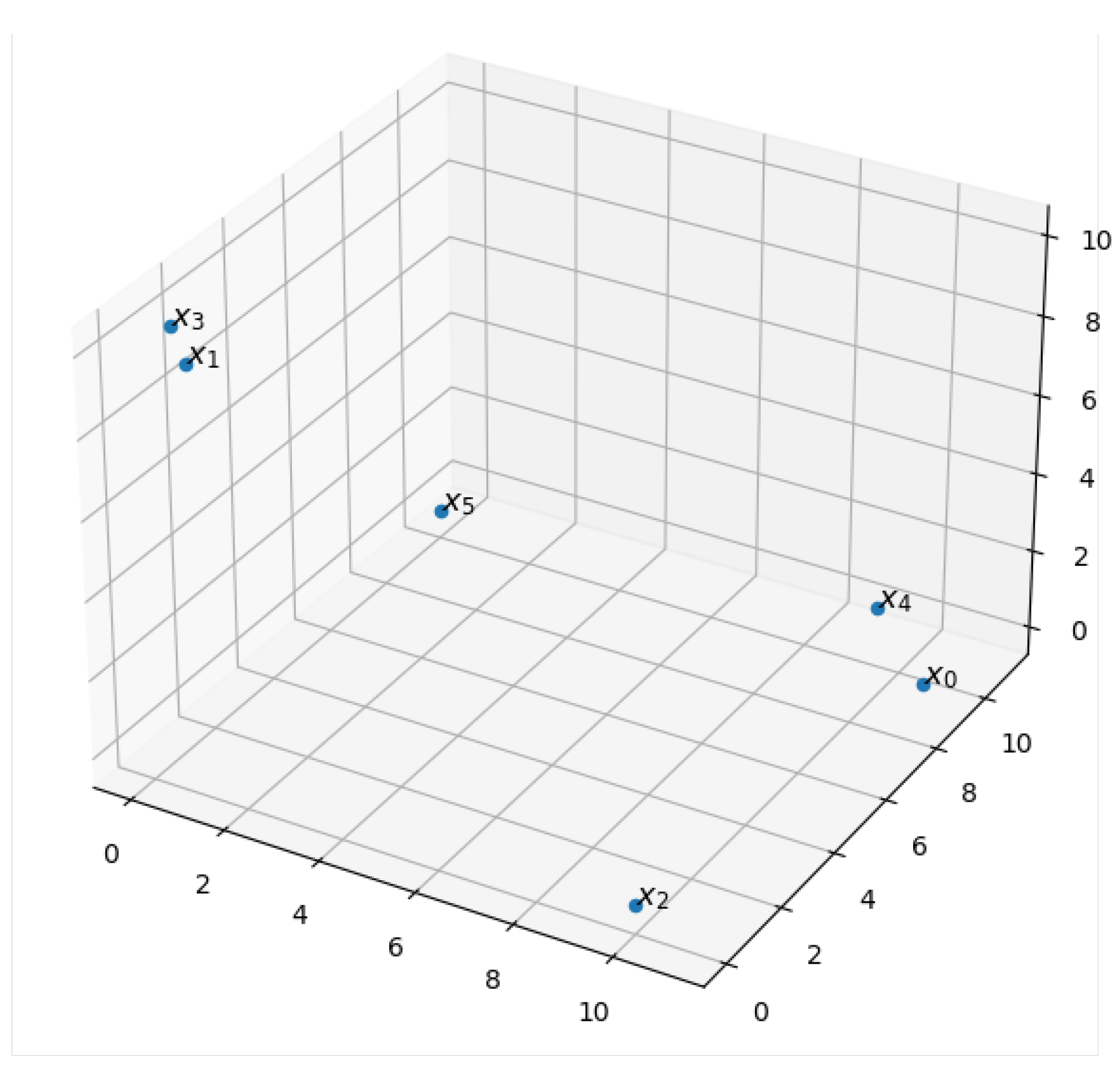
2.2.1. Geometric Features

In order to describe the geometry of the data-set $\mathbb{M}$, we first identify four types of geometrical features associated with $\mathbb{M}$:

• A vertex $\left[{\mathbf{x}}_m\right]$ is generated by an individual point ${\mathbf{x}}_m\in \mathbb{M}$;
• A segment $[{\mathbf{x}}_m,{\mathbf{x}}_n]$ joins two vertex $\left[{\mathbf{x}}_m\right],\left[{\mathbf{x}}_n\right]\in \mathbb{M}$

  $$[{\mathbf{x}}_m,{\mathbf{x}}_n]:=\left\{\mathbf{x}\in {\mathbb{R}}^3:\mathbf{x}=\lambda {\mathbf{x}}_m+(1-\lambda ){\mathbf{x}}_n\mathrm{where}0\le \lambda \le 1\right\};$$
• A triangle is generated by three different vertexes $\left[{\mathbf{x}}_m\right],\left[{\mathbf{x}}_n\right],\left[{\mathbf{x}}_l\right]\in \mathbb{M}$, such that ${\mathbf{x}}_m-{\mathbf{x}}_n$ and ${\mathbf{x}}_m-{\mathbf{x}}_l$ are linearly independent, and then:

  $$[{\mathbf{x}}_m,{\mathbf{x}}_n,{\mathbf{x}}_l]:=\left\{\mathbf{x}\in {\mathbb{R}}^3:\mathbf{x}={\lambda }_m{\mathbf{x}}_m+{\lambda }_n{\mathbf{x}}_n+{\lambda }_l{\mathbf{x}}_l\right\},$$

  where ${\lambda }_m,{\lambda }_n$ and ${\lambda }_l$ are the barycentric coordinates, with ${\lambda }_m+{\lambda }_n+{\lambda }_l=1$;
• A tetrahedron is generated by four different vertices $\left[{\mathbf{x}}_m\right],\left[{\mathbf{x}}_n\right],\left[{\mathbf{x}}_l\right],\left[{\mathbf{x}}_p\right]\in \mathbb{M}$, such that ${\mathbf{x}}_m-{\mathbf{x}}_n$, ${\mathbf{x}}_m-{\mathbf{x}}_l$, and ${\mathbf{x}}_m-{\mathbf{x}}_p$ are linearly independent, and then:

  $$[{\mathbf{x}}_m,{\mathbf{x}}_n,{\mathbf{x}}_l,{\mathbf{x}}_p]:=\left\{\mathbf{x}\in {\mathbb{R}}^3:\mathbf{x}={\lambda }_m{\mathbf{x}}_m+{\lambda }_n{\mathbf{x}}_n+{\lambda }_l{\mathbf{x}}_l+{\lambda }_p{\mathbf{x}}_p\right\},$$

  where ${\lambda }_m,{\lambda }_n$, ${\lambda }_l$ and ${\lambda }_p$ are the barycentric coordinates, with ${\lambda }_m+{\lambda }_n+{\lambda }_l+{\lambda }_p=1$.

The vertices represent the dimension-0 features, segments the dimension-1 features, and triangles the dimension-2 features and tetrahedron dimension-3 features.

2.2.2. Features’ Filtration

To describe the appearance and disappearance of the features of $\mathbb{M}$ across different scales, we consider the so-called Alpha Filtration. For that purpose, an interval $[{\alpha }_{min},{\alpha }_{max}]$ is considered. It reflects the smallest features’ scale, in our case ${\alpha }_{min}=0$ (the vertex) and the largest one ${\alpha }_{max}$ representing the largest distance between points of $\mathbb{M}$.

The features of $\mathbb{M}$ considered here are elements of the Simplicial complex associated with $\mathbb{M}$, noted $S\left(\mathbb{M}\right)$, and constructed from the finite cells of the the Delaunay Triangulation of the set of points in $\mathbb{M}$. The elements of $S\left(\mathbb{M}\right)$ are the geometric features of $\mathbb{M}$ i.e., tetrahedrons, triangles, edges, and vertices.

In order to describe efficiently the elements of the Simplicial complex $S\left(\mathbb{M}\right)$, and map a set of d-dimensional simplices to a set of $(d-1)$-dimensional simplices, we construct a finite sequence of sets of d-dimensional simplices, denoted by $S_d\left(\mathbb{M}\right)$, $d=0,1,2,3$.

Set $S_0\left(\mathbb{M}\right):=\{\left[x_m\right]:x_m\in \mathbb{M}\};$ then, the simplices in $S_d\left(\mathbb{M}\right)$ for each $d=1,2,3$ are obtained from the simplices in $S_{d-1}\left(\mathbb{M}\right)$ taking into account the following two properties:

• For every simplex in $S_d\left(\mathbb{M}\right)$, the $(d-1)$-dimensional simplices forming it are in $S_{d-1}\left(\mathbb{M}\right)$ (e.g., a triangle is in $S_2\left(\mathbb{M}\right)$ and its three edges are in $S_1\left(\mathbb{M}\right)$);
• If two simplices in $S_d\left(\mathbb{M}\right)$ have a common element $\sigma$, then there exists $0\le l\le (d-1)$ such that $\sigma \in S_l\left(\mathbb{M}\right)$.

Given the scale values ${\left({\alpha }_j\right)}_{j=0}^m$, the Alpha Filtration is then a non-decreasing sequence describing the evolution of the features of the simplicial complex $S\left(\mathbb{M}\right)$ at each scale ${\alpha }_j$, and computed as follows:

• First, the filtration value of each tetrahedron is computed as the circumradius of the tetrahedron if its circumsphere is empty, and as the minimum of the filtration values of the triangles that are within the circumsphere otherwise.
• Similarly, the filtration value of each triangle is computed as the circumradius of the triangle if the circumcircle is empty, and as the minimum of the filtration values of the segments that are within the circumcircle otherwise.
• Then, the filtration value of each segment is computed as its circumradius.
• Finally, the filtration value of the vertices is set to 0.

The discrete values used for the radii are the ${\alpha }_j$, and all simplices that have a filtration value larger than ${\alpha }_{max}$ are discarded.

The time complexity of the algorithm is $\mathcal{O}\left(n^2\right)$. The choice of the Alpha Filtration was motivated by its relatively much smaller size compared to other filtrations. A detailed definition and implementation are provided in [17,18].

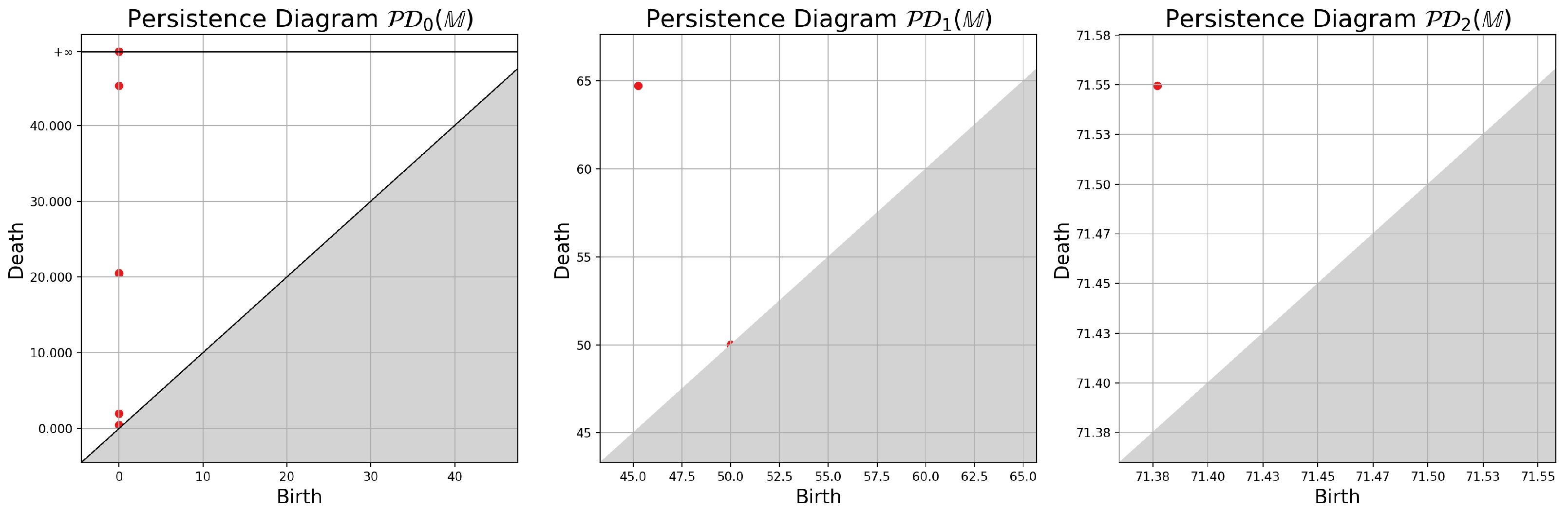
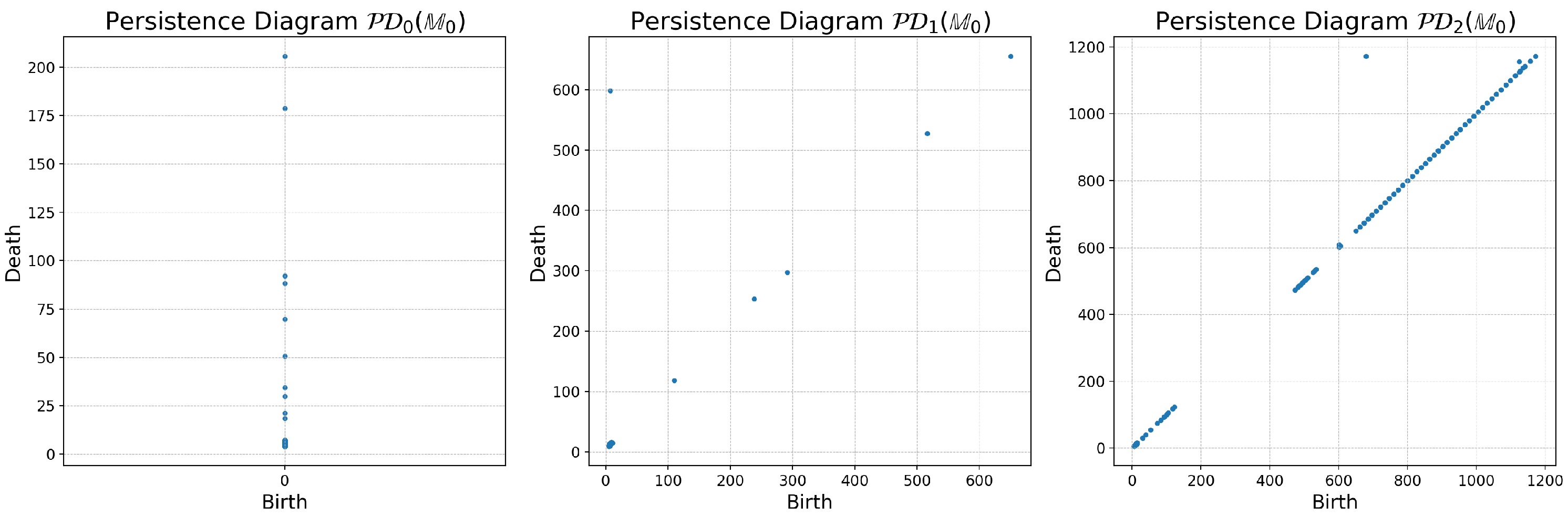
2.2.3. Persistence Diagrams

In order to have a more exhaustive view on how the features are changing across different scales, the appearance and disappearance of each feature within the filtration are tracked and coded into the Homology Groups $H_k\left(\mathbb{M}\right)$, where $k=0,1,2,3$ is the homology dimension.

The elements of a Homology Group $H_k\left(\mathbb{M}\right)$ are classes of chains of simplices (“packets”) $\sigma \in S_k\left(\mathbb{M}\right),$ that is, simplices sharing faces, edges, or vertices. It can be seen as a connected component of the intersection of $\mathbb{M}$ with a k-dimensional linear subspace of ${\mathbb{R}}^3$. The use of Homology Groups allows for performing algebraic operations over their elements.

Given a Homology Group, we can now define how to track the appearance of the features across different scales, by defining the Homology Group at a scale $\alpha$, $H_k^{\alpha }\left(\mathbb{M}\right)$. It represents the classes of simplices as described previously, but taken from $S_k^{\alpha }\left(\mathbb{M}\right)$. That is, the elements of $S_k\left(\mathbb{M}\right)$ with a filtration value lesser that $\alpha$.

This approach is known as the Persistent Homology. It allows for quantifying the appearance and disappearance of the features across the different scales and dimensions:

• The birth scale $b_{\gamma }$ of the feature $\gamma$ at homology k

  $$b_{\gamma }=\underset{0\le j\le m}{min}\{{\alpha }_j:\gamma \in H_k^{{\alpha }_j}\}$$
• The death scale $d_{\gamma }$ of the feature $\gamma$ at homology k

  $$d_{\gamma }=\underset{0\le j\le m}{max}\{{\alpha }_j:\gamma \in H_k^{{\alpha }_j}\}$$

The birth scale represents the value at which the feature appeared in the filtration by combining lower dimensional simplices to form it. Conversely, the death scale represents the value at which the feature disappeared in the filtration by being combined into a higher dimensional feature. For example, if a vertex is part of a segment, then the death scale of the vertex is exactly the birth scale of the associated segment.

Note that, by definition, vertices always have a zero birth scale, while tetrahedrons always have an infinite death scale (in the numerical results, we removed the infinite values for computation purposes). Given that our data points $\mathbb{M}$ are embedded in ${\mathbb{R}}^3$, we will only track up to the dimension-2 features, thus the definition of $S\left(\mathbb{M}\right)$ with $k=0,1,2$. More generally, if the data points are embedded in a d-dimensional manifold, the persistent homology can be computed up to dimension $d-1$.

Finally, the persistence of the features throughout the scales can be represented by the so-called Persistence Diagram of $\mathbb{M}$, defined at dimension-k from

$${\mathcal{PD}}_k\left(\mathbb{M}\right)=\{(b_{\gamma },d_{\gamma }):\gamma \in H_k\},$$

where $b_{\gamma }$ and $d_{\gamma }$ are the birth and death scales of a feature $\gamma$ at homology k.

The surface $\mathbb{M}$ persistence diagrams $\mathcal{PD}\left(\mathbb{M}\right)$ read

$$\mathcal{PD}\left(\mathbb{M}\right)=\{{\mathcal{PD}}_0\left(\mathbb{M}\right),{\mathcal{PD}}_1\left(\mathbb{M}\right),{\mathcal{PD}}_2\left(\mathbb{M}\right)\}.$$

2.2.4. Illustrating the Concepts on an Example

We illustrate the computational aspects of the Alpha Filtration on a simple example, consisting of six points in ${\mathbb{R}}^3$, as shown in Figure 3:

$$\begin{array}{cc}\hfill \mathbb{M}=\{& {\mathbf{x}}_0=(1.1,0.9,0),{\mathbf{x}}_1=(0.1,0,1),{\mathbf{x}}_2=(0,0,0),\hfill \\ \hfill & {\mathbf{x}}_3=(0,0.1,1),{\mathbf{x}}_4=(0.9,1.1,0),{\mathbf{x}}_5=(0,1,0)\}\hfill \end{array}$$

The filtration values are computed and presented below in

Table 1. Alpha Filtration of $\mathbb{M}$.

$\mathit{\alpha }$	${\mathit{S}}_0^{\mathit{\alpha }}$	${\mathit{S}}_1^{\mathit{\alpha }}$	${\mathit{S}}_2^{\mathit{\alpha }}$	${\mathit{S}}_3^{\mathit{\alpha }}$
0.00	$\left[x_0\right],\left[x_1\right],\left[x_2\right]$	-	-	-
	$\left[x_3\right],\left[x_4\right],\left[x_5\right]$
0.50	$\left[x_0\right],\left[x_1\right],\left[x_2\right]$	$[x_1,x_3]$	-	-
	$\left[x_3\right],\left[x_4\right],\left[x_5\right]$
2.00	$\left[x_0\right],\left[x_1\right],\left[x_2\right]$	$[x_1,x_3],[x_0,x_4]$	-	-
	$\left[x_3\right],\left[x_4\right],\left[x_5\right]$
20.50	$\left[x_0\right],\left[x_1\right],\left[x_2\right]$	$[x_1,x_3],[x_0,x_4]$	-	-
	$\left[x_3\right],\left[x_4\right],\left[x_5\right]$	$[x_0,x_2],[x_4,x_5]$
45.25	$\left[x_0\right],\left[x_1\right],\left[x_2\right]$	$[x_1,x_3],[x_0,x_4]$	-	-
	$\left[x_3\right],\left[x_4\right],\left[x_5\right]$	$[x_0,x_2],[x_4,x_5]$
		$[x_1,x_2],[x_3,x_5]$
50.00	$\left[x_0\right],\left[x_1\right],\left[x_2\right]$	$[x_1,x_3],[x_0,x_4]$	-	-
	$\left[x_3\right],\left[x_4\right],\left[x_5\right]$	$[x_0,x_2],[x_4,x_5]$
		$[x_1,x_2],[x_3,x_5]$
		$[x_2,x_5]$
50.02	$\left[x_0\right],\left[x_1\right],\left[x_2\right]$	$[x_1,x_3],[x_0,x_4]$	-	-
	$\left[x_3\right],\left[x_4\right],\left[x_5\right]$	$[x_0,x_2],[x_4,x_5]$
		$[x_1,x_2],[x_3,x_5]$
		$[x_2,x_5],[x_2,x_4]$
64.73	$\left[x_0\right],\left[x_1\right],\left[x_2\right]$	$[x_1,x_3],[x_0,x_4]$	$[x_1,x_2,x_5],[x_1,x_3,x_5]$	-
	$\left[x_3\right],\left[x_4\right],\left[x_5\right]$	$[x_0,x_2],[x_4,x_5]$
		$[x_1,x_2],[x_3,x_5]$
		$[x_2,x_5],[x_2,x_4]$
		$[x_1,x_5]$
70.64	$\left[x_0\right],\left[x_1\right],\left[x_2\right]$	$[x_1,x_3],[x_0,x_4]$	$[x_1,x_2,x_5],[x_1,x_3,x_5]$	-
	$\left[x_3\right],\left[x_4\right],\left[x_5\right]$	$[x_0,x_2],[x_4,x_5]$	$[x_0,x_1,x_2],[x_3,x_4,x_5]$
		$[x_1,x_2],[x_3,x_5]$
		$[x_2,x_5],[x_2,x_4]$
		$[x_1,x_5],[x_0,x_1]$
		$[x_3,x_4]$
71.38	$\left[x_0\right],\left[x_1\right],\left[x_2\right]$	$[x_1,x_3],[x_0,x_4]$	$[x_1,x_2,x_5],[x_1,x_3,x_5]$	-
	$\left[x_3\right],\left[x_4\right],\left[x_5\right]$	$[x_0,x_2],[x_4,x_5]$	$[x_0,x_1,x_2],[x_3,x_4,x_5]$
		$[x_1,x_2],[x_3,x_5]$	$[x_0,x_1,x_4],[x_1,x_3,x_4]$
		$[x_2,x_5],[x_2,x_4]$
		$[x_1,x_5],[x_0,x_1]$
		$[x_3,x_4],[x_1,x_4]$
71.55	$\left[x_0\right],\left[x_1\right],\left[x_2\right]$	$[x_1,x_3],[x_0,x_4]$	$[x_1,x_2,x_5],[x_1,x_3,x_5]$	$[x_0,x_1,x_2,x_4]$
	$\left[x_3\right],\left[x_4\right],\left[x_5\right]$	$[x_0,x_2],[x_4,x_5]$	$[x_0,x_1,x_2],[x_3,x_4,x_5]$	$[x_1,x_2,x_4,x_5]$
		$[x_1,x_2],[x_3,x_5]$	$[x_0,x_1,x_4],[x_1,x_3,x_4]$	$[x_1,x_3,x_4,x_5]$
		$[x_2,x_5],[x_2,x_4]$	$[x_1,x_2,x_4],[x_1,x_4,x_5]$
		$[x_1,x_5],[x_0,x_1]$
		$[x_3,x_4],[x_1,x_4]$

:

We can then track the birth and death of the features and compute the persistence diagrams $\mathcal{PD}\left(\mathbb{M}\right)$, as shown in Figure 4.

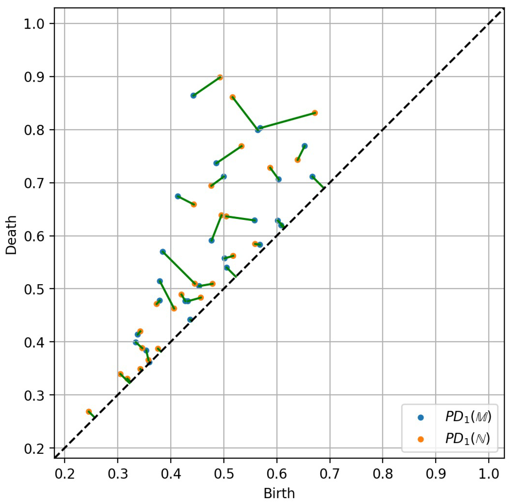
2.2.5. Matching Persistence Diagrams

Consider two data-sets ${\mathbb{M}}_r$ and ${\mathbb{M}}_s$ representing two deformed configurations of the same surface. A matching between two persistence diagrams with the same number of features, ${\mathcal{PD}}_k\left({\mathbb{M}}_r\right)$ and ${\mathcal{PD}}_k\left({\mathbb{M}}_s\right)$, for $k=0,1,2$, is a bijective map ${\psi }^k$ that reads:

$${\psi }^k:{\mathcal{PD}}_k\left({\mathbb{M}}_r\right)⟶{\mathcal{PD}}_k\left({\mathbb{M}}_s\right),$$

such that $\forall \gamma =(b,d)\in {\mathcal{PD}}_k\left({\mathbb{M}}_r\right)$,

$$\begin{array}{cc}\hfill {\psi }^k\left(\gamma \right)& =({\psi }_1^k\left(b\right),{\psi }_2^k\left(d\right))\hfill \\ \hfill & =(b^{\prime },d^{\prime })\in {\mathcal{PD}}_k\left({\mathbb{M}}_s\right).\hfill \end{array}$$

The map ${\psi }^k$ associates each feature from ${\mathcal{PD}}_k\left({\mathbb{M}}_r\right)$ to a feature from ${\mathcal{PD}}_k\left({\mathbb{M}}_s\right)$. The Optimal Matching between ${\mathcal{PD}}_k\left({\mathbb{M}}_r\right)$ and ${\mathcal{PD}}_k\left({\mathbb{M}}_s\right)$ is a matching ${\widehat{\psi }}^k$

$${\widehat{\psi }}^k:{\mathcal{PD}}_k\left({\mathbb{M}}_r\right)⟶{\mathcal{PD}}_k\left({\mathbb{M}}_s\right),$$

minimizing the transport cost ${\mathcal{C}}^k$ to move the features from ${\mathcal{PD}}_k\left({\mathbb{M}}_r\right)$ to ${\mathcal{PD}}_k\left({\mathbb{M}}_s\right)$:

$$\begin{array}{cc}\hfill {\mathcal{C}}_{\mathtt{min}}^k=& \sum _{\gamma \in {\mathcal{PD}}_k\left({\mathbb{M}}_r\right)}{\parallel \gamma -{\widehat{\psi }}^k\left(\gamma \right)\parallel }_2\hfill \\ \hfill =& \sum _{(b,d)\in {\mathcal{PD}}_k\left({\mathbb{M}}_r\right)}{\parallel \left(b-{\widehat{\psi }}_1^k\left(b\right),d-{\widehat{\psi }}_2^k\left(d\right)\right)\parallel }_2\hfill \\ \hfill =& \sum _{(b,d)\in {\mathcal{PD}}_k\left({\mathbb{M}}_r\right)}\sqrt{{\left(b-{\widehat{\psi }}_1^k\left(b\right)\right)}^2+{\left(d-{\widehat{\psi }}_2^k\left(d\right)\right)}^2}.\hfill \end{array}$$

When ${\mathbb{M}}_r$ is the reference surface, and ${\mathbb{M}}_s$ is any deformed surface resulting from ${\mathbb{M}}_r$, the optimal matching ${\widehat{\psi }}^k$ represents and quantifies the deformation from a topological viewpoint, at each dimension $k=0,1,2$.

We note that, in our case considered here, the diagrams have all been reduced to their top 3000 persistence values, making the bijective matching possible. In the case of diagrams with a different number of points, a partial matching is rather considered.

The optimal matching is computed using a combinatorial optimization procedure, where the points in both diagrams are matched while minimizing the transport cost function defined above. A graphical representation of the matching is shown in Figure 5.

2.2.6. Multi-Scale Topological Measure of Surface Deformation

It is now possible to measure the degree of deformation from one data-set to another. For that purpose, consider two data-sets ${\mathbb{M}}_r$ and ${\mathbb{M}}_s$ representing two deformed states of the same surface, and a finite sequence of ${\left({\alpha }_j\right)}_{j=0}^m$. Then, for $k=0,1,2$, the k-distance between ${\mathcal{PD}}_k\left({\mathbb{M}}_r\right)$ and ${\mathcal{PD}}_k\left({\mathbb{M}}_s\right)$ reads

$$W_k\left({\mathcal{PD}}_k\left({\mathbb{M}}_r\right),{\mathcal{PD}}_k\left({\mathbb{M}}_s\right)\right)=\sum _{(b,d)\in {\mathcal{PD}}_k\left({\mathbb{M}}_r\right)}\sqrt{{\left(b-{\widehat{\psi }}_1^k\left(b\right)\right)}^2+{\left(d-{\widehat{\psi }}_2^k\left(d\right)\right)}^2},$$

where ${\widehat{\psi }}^k$ is the optimal matching between ${\mathcal{PD}}_k\left({\mathbb{M}}_r\right)$ and ${\mathcal{PD}}_k\left({\mathbb{M}}_s\right)$. An efficient computation of that distance $W_k$, known as the Wasserstein Distance, is performed using the kernel linearization presented in Algorithm 2 of reference [19].

The Multi-Scale Topological Distance between ${\mathbb{M}}_r$ and ${\mathbb{M}}_s$ reads

$$\mathsf{\Omega }({\mathbb{M}}_r,{\mathbb{M}}_s)=\sqrt{{\omega }_0^2+{\omega }_1^2+{\omega }_2^2},$$

where ${\omega }_k=W_k\left({\mathcal{PD}}_k\left({\mathbb{M}}_r\right),{\mathcal{PD}}_k\left({\mathbb{M}}_s\right)\right),k=0,1,2$.

2.2.7. Comparing Tropological Descriptions of Deformed Surfaces

Consider now our collection $\{{\mathbb{M}}_0,{\mathbb{M}}_1,\dots ,{\mathbb{M}}_{\mathcal{M}}\}$ of data-sets, consisting of the reference surface ${\mathbb{M}}_0$ and $\mathcal{M}=102$ deformed surfaces ${\mathbb{M}}_r$, $r=1,\dots ,\mathcal{M}$.

By using the previously defined metric $\mathsf{\Omega }$, we can measure each surface deformation with respect to the reference one, such that $\forall r\in \{1,\dots ,\mathcal{M}\}$ and we have

$${\mathsf{\Omega }}_r=\mathsf{\Omega }({\mathbb{M}}_0,{\mathbb{M}}_r)=\sqrt{{\omega }_{0,r}^2+{\omega }_{1,r}^2+{\omega }_{2,r}^2},$$

where $\forall r\in \{1,\dots ,\mathcal{M}\},\forall k\in \{0,1,2\}$, we denote

$${\omega }_{k,r}=W_k\left({\mathcal{PD}}_k\left({\mathbb{M}}_0\right),{\mathcal{PD}}_k\left({\mathbb{M}}_r\right)\right).$$

The measure ${\mathsf{\Omega }}_r$ enables clustering the different surfaces ($6\times 17$, 17 being the number of structural configurations, each one related to a particular value of the thickness) into six clusters.

2.3. Modal Assurance Criterion

One of the most popular tools for the quantitative comparison of modal vectors is the Modal Assurance Criterion (MAC) [13]. The MAC criterion is a statistical indicator that is quite sensitive to large differences of the eigenmodes.

In our case, each mode ${\mathbb{M}}_r$ ($r=1,\dots ,\mathcal{M}$) is decomposed in its linear and angular components (with respect to the three coordinate axes), resulting in the six vectors ${\left\{{\Psi }_c^r\right\}}_{1\le c\le 6}$.

The $\mathtt{MAC}$ of two surfaces ${\mathbb{M}}_r$ and ${\mathbb{M}}_s$ is then computed according to

$$\mathtt{MAC}({\mathbb{M}}_r,{\mathbb{M}}_s)=\frac{{\sum }_{c=1}^6{\left({\Psi }_c^r·{\Psi }_c^s\right)}^2}{\left({\sum }_{c=1}^6{\left({\Psi }_c^r\right)}^2\right)\left({\sum }_{c=1}^6{\left({\Psi }_c^r\right)}^2\right)}.$$

The $\mathtt{MAC}$ takes values between 0 (representing no consistent correspondence) and 1 (representing a consistent correspondence). Values larger than $0.9$ indicate consistent correspondence, whereas small values indicate poor resemblance of the two eigenmodes.

Thus, considering the six modes related to two different structures (with two different thicknesses), it is now possible to compute the so-called MAC matrix $\mathbf{M}$ to compare the modes and identify resemblances or discrepancies.

The MAC matrix $\mathbf{M}$ becomes diagonal dominant when modes are well ordered, whereas the loss of that diagonal dominancy informs on eventual permutations. In order to apply the MAC criterion in the case study addressed in the present paper, the first reduced modal basis consisting of the six modes related to the first thickness will be compared with the six modes of all the other configurations, the remaining 16 thickness choices.

3. Results

3.1. Topological Modes Identification

By applying the methodology described in Section 2.2 to the surface data-sets, by first computing the Alpha Filtration, we obtain the persistence diagrams ${\left\{{\mathcal{PD}}_k\left({\mathbb{M}}_r\right)\right\}}_{r=0}^{\mathcal{M}=102}$, with the ones associated with the reference surface shown in Figure 6.

The multi-scale distance defined in Section 2.2.6 and here associated with each surface ${\left\{{\mathsf{\Omega }}_r\right\}}_{r=1}^{\mathcal{M}=102}$ is then computed, and reported in

Table 2. Multi-scale topological distance of the six deformed surfaces related to the six most significant deformation modes, of the 17 choices of the structure thickness with respect to the reference undeformed surface.

Case	1st surf.	2nd surf.	3rd surf.	4th surf.	5th surf.	6th surf.
01	2828	3742	6012	6281	7070	7314
02	3839	4341	5160	5269	8299	9530
03	3540	4003	4702	5536	6436	8023
04	2971	3762	5883	7481	7429	9314
05	3062	3762	5437	6156	9865	10,307
06	4852	5239	7294	8336	8237	9585
07	3482	4411	6095	6882	9319	10,627
08	3392	3684	5903	6710	9273	9438
09	4648	5436	7986	7707	10,415	9406
10	4425	4267	5583	5811	9620	9163
11	3256	3722	4782	4888	5840	8064
12	2993	3750	5551	6885	7135	8474
13	4281	4862	7127	8230	8170	9687
14	4367	5004	7140	7036	8285	8008
15	4937	5396	6484	6446	9323	10,031
16	3184	3941	4907	4965	7205	8869
17	2957	3652	5652	6021	7659	7571

.

This multi-scale topological distance is then used to order the deformed surfaces to retain in each column of

Table 3. Surface ordering. Numbers in red indicate the permutation that must be performed in order to align surfaces with respect to its shape.

Case	1st surf.	2nd surf.	3rd surf.	4th surf.	5th surf.	6th surf.
01	1	2	3	4	5	6
02	1	2	3	4	5	6
03	1	2	3	4	5	6
04	1	2	3	5	4	6
05	1	2	3	4	5	6
06	1	2	3	5	4	6
07	1	2	3	4	5	6
08	1	2	3	4	5	6
09	1	2	4	3	6	5
10	2	1	3	4	6	5
11	1	2	3	4	5	6
12	1	2	3	4	5	6
13	1	2	3	5	4	6
14	1	2	4	3	6	5
15	1	2	4	3	5	6
16	1	2	3	4	5	6
17	1	2	3	4	6	5

those exhibiting a shape resemblance. From Table 2 and Table 3, the surfaces have been sorted using the values of Table 2, and their sorted order displayed in Table 3. The goal is to have the surfaces labeled from the least to the most deformed, according to our measure of deformation. In Table 3, numbers in red indicate surface (modes) permutations that have been made in order to classify all the shapes.

3.2. MAC Identification

Using the MAC criterion described in Section 2.3, we compute the MAC matrices comparing the model reduced basis (of the first thickness choice) with the remaining 16 reduced modal bases for the other thickness choices, and the results are reported in Figure 7.

4. Discussion and Conclusions

Labelling the surfaces as reported in Table 3 aims at classifying them according their shape induced by their deformation. The greater the value of the topological metric $\mathsf{\Omega }$, the more deformed the surfaces are. The surface discrepancies are quantified from the transport cost related to the matching of the topological features that the deformed meshes express, through the different scales and dimension.

The value of $\mathsf{\Omega }$ can be interpreted as a level of topological deformation for a certain deformed mesh on the deformed surface compared with the undeformed mesh and surface. Thus, labels 1 to 6 in the case addressed here express the magnitude of the surface deformation. Figure 8 depicts the six ordered deformed surfaces for one particular case (structure with a given thickness).

By inspecting Table 3, it can be noticed that the surface label usually matches the order of the eigenmodes provided by the eigenproblem solution. However, when modifying the structure thickness, some shapes that were important for a given thickness can be now more or less significant and the order of apparition in the eigenproblem differs. Thus, a permutation must be performed for ordering the modes with respect to their intrinsic shapes, here evaluated by using a metric based on topological concepts.The MAC matrices displayed in Figure 7 show similar tendencies, as the modes are globally consistent with their labels.

The presented topology-based framework for measuring surface deformations seems a very pertinent, powerful, and intrinsic way of quantifying, characterizing, and analyzing the deformation modes of structures. The strength of the framework relies on both the topology description of the surface at multiple scales, and the proposed measure based on the optimal matching of the features, to detect how each feature of the surface was deformed.

References

1. Clough, R.W.; Penzien, J. Dynamics of structures; Civil Engineering Series; McGraw-Hill: New York, NY, USA, 1993. [Google Scholar]
2. Newmark, N.M. A method of computation for structural dynamics. J. Eng. Mech. Div. 1959, 85, 67–94. [Google Scholar] [CrossRef]
3. Bathe, J. Conserving energy and momentum in nonlinear dynamics: A simple implicit time integration scheme. Comput. Struct. 2007, 85, 437–445. [Google Scholar] [CrossRef]
4. Germoso, C.; Duval, J.L.; Chinesta, F. Harmonic-Modal Hybrid Reduced Order Model for the Efficient Integration of Non-Linear Soil Dynamics. Appl. Sci. 2020, 10, 6778. [Google Scholar] [CrossRef]
5. Malik, M.H.; Borzacchiello, D.; Aguado, J.V.; Chinesta, F. Advanced parametric space-frequency separated representations in structural dynamics: A harmonic–modal hybrid approach. Comptes Rendus MéCanique 2018, 346, 590–602. [Google Scholar] [CrossRef]
6. Quaranta, G.; Argerich, C.; Ibañez, R.; Duval, J.L.; Cueto, E.; Chinesta, F. From linear to nonlinear PGD-based parametric structural dynamics. Comptes Rendus MéCanique 2019, 347, 445–454. [Google Scholar] [CrossRef]
7. Boucinha, L.; Gravouil, A.; Ammar, A. Space-time proper generalized decompositions for the resolution of transient elastodynamic models. Comput. Methods Appl. Mech. Eng. 2013, 255, 67–88. [Google Scholar] [CrossRef] [Green Version]
8. Ladeveze, P. The large time increment method for the analyze of structures with nonlinear constitutive relation described by internal variables. CR Acad. Sci. Paris 1989, 309, 1095–1099. [Google Scholar]
9. Ladeveze, P.; Arnaud, L.; Rouch, P.; Blanze, C. The variational theory of complex rays for the calculation of medium-frequency vibrations. Engrg. Comp. 1999, 18, 193–214. [Google Scholar] [CrossRef] [Green Version]
10. Gonzalez, D.; Cueto, E.; Chinesta, F. Real-Time Direct Integration of Reduced Solid Dynamics Equations. Int. J. Numer. Methods Eng. 2014, 99/9, 633–653. [Google Scholar] [CrossRef] [Green Version]
11. Chinesta, F.; Leygue, A.; Bordeux, F.; Aguado, J.V.; Cueto, E.; Gonzalez, D.; Alfaro, I.; Huerta, A. Parametric PGD based computational vademecum for efficient design, optimization and control. Arch. Comput. Methods Eng. 2013, 20/1, 31–59. [Google Scholar] [CrossRef]
12. Sancarlos, A.; Champaney, V.; Duval, J.L.; Cueto, E.; Chinesta, F. PGD-based advanced nonlinear multiparametric regressions for constructing metamodels at the scarce-data limit. arXiv 2021, arXiv:2103.05358. [Google Scholar]
13. Pastora, M.; Bindaa, M.; Harcarika, T. Modal Assurance Criterion. Procedia Eng. 2012, 48, 543–548. [Google Scholar] [CrossRef]
14. Louis, M.; Bône, A.; Charlier, B.; Durrleman, S. Parallel Transport in Shape Analysis: A Scalable Numerical Scheme. In International Conference on Geometric Science of Information; Lecture Notes in Computer Science; Springer: Cham, Switzerland, 2017; Volume 10589. [Google Scholar]
15. Frahi, T.; Argerich, C.; Yun, M.; Falco, A.; Barasinski, A.; Chinesta, F. Tape surfaces characterization with persistence images. AIMS Mater. Sci. 2020, 7, 364–380. [Google Scholar] [CrossRef]
16. Frahi, T.; Chinesta, F.; Falco, A.; Badias, A.; Cueto, E.; Choi, H.Y.; Han, M.; Duval, J.L. Empowering Advanced Driver-Assistance Systems from Topological Data Analysis. Mathematics 2021, 9, 634. [Google Scholar] [CrossRef]
17. Edelsbrunner, H.; Harer, J.L. Computational Topology: An Introduction; American Mathematical Society: Providence, RI, USA, 2009. [Google Scholar]
18. GUDHI Project. GUDHI User and Reference Manual. GUDHI Editorial Board. 2021. Available online: https://gudhi.inria.fr/doc/3.4.1/ (accessed on 3 July 2021).
19. Carrière, M.; Cuturi, M.; Oudot, S. Sliced Wasserstein Kernel for Persistence Diagrams. In Proceedings of the 34th International Conference on Machine Learning, Sydney, Australia, 6–11 August 2017. PMLR 70:664-673. [Google Scholar]
Figure 1. Reference undeformed structure (left) and its deformed counterpart (right) when a given deformation mode applied on the reference one.
Applsci 11 06554 g001
Figure 2. Reference surface (left) and nodes distribution on it (right).
Applsci 11 06554 g002
Figure 3. Example of data points M .
Applsci 11 06554 g003
Figure 4. Persistence diagrams PD ( M ) .
Applsci 11 06554 g004
Figure 5. Optimal matching of two persistence diagrams PD 1 ( M ) and PD 1 ( N ) .
Applsci 11 06554 g005
Figure 6. Persistence diagrams associated with the reference surface, PD k ( M 0 ) , for k = 0 (left), k = 1 (center) and k = 2 (right).
Applsci 11 06554 g006
Figure 7. Modal Assurance Criterion matrices when comparing the model reduced basis—RB— (of the first thickness choice) with the remaining 16 reduced modal bases for the other thickness choices.
Applsci 11 06554 g007
Figure 8. (top-left) First mode; (top-right) Second mode; (middle-left) Third mode; (middle-right) Fourth mode; (bottom-left) Fifth mode; and (bottom-right) Sixth mode.
Applsci 11 06554 g008