1. Introduction
Data mining is determined as an important step in the knowledge discovery process. It has become an active research domain due to the presence of huge collections of digital data that need to be explored and transformed into useful patterns. The main role of data mining is to develop methods that assist in finding potentially useful hidden patterns in huge data collections [
1]. In data mining techniques such as classification, preprocessing of data has a great influence on the goodness of discovered patterns and the efficiency of machine learning classifiers [
1,
2]. Feature selection (FS) is one of the main preprocessing techniques to discover and retain informative features and eliminate noisy and irrelevant ones. Selecting the optimal or near-optimal subset of given features will enhance the performance of the classification models and reduce the computational cost [
2,
3,
4].
Based on the evaluation criteria of the selected features subset, FS approaches are classified into two classes: filter and wrapper approaches [
3]. Filter techniques depend on scoring matrices such as chi-square and information gain to estimate the quality of the picked subset of features. More accurately, in filter approaches, a filter approach (e.g., chi-square) is used to rank the features, and then the only ones that have weights greater than or equal to a predefined threshold are retained. In contrast, wrapper approaches mainly consider a machine learning classifier such as K-Nearest Neighbors (KNN) or Support Vector Machines (SVM) to evaluate the feature subset.
Another aspect for categorizing FS methods is based on the selection mechanism that is used to explore the feature space, searching for the most informative features. The search algorithm task is to generate subsets of features, and then the machine learning algorithm is applied to assess the generated subsets of features to find the optimal one [
4,
5,
6]. Compared to filter approaches, wrappers have superior performance, especially in terms of accuracy since it considers the dependencies between features in the dataset, while filter FS may ignore such relations [
7]. Although, filter FS is better than wrapper FS in terms of computational cost [
4].
Commonly, for a wide range of data mining applications, reaching the optimal subset of features is a challenging task. The size of the search space grows exponentially with respect to the number of features (i.e.,
possible subsets can be generated for a dataset with
k features). Accordingly, FS is an intractable NP-hard optimization problem in which exhaustive search and even conventional exact optimization methods are impractical. For that reason, the FS domain has been extensively investigated by many researchers [
5,
8]. For example, in [
9], an improved version of the binary Particle Swarm Optimization (PSO) algorithm was introduced for the FS problem. An unsupervised FS approach based on Ant Colony Optimization (ACO) was proposed by [
10]. Moreover, an FS technique that hybrids Genetic Algorithm (GA) and PSO was introduced in [
11]. Finally, a binary variant of the hybrid Grey Wolf Optimization (GWO) and PSO is presented in [
12] to tackle the FS problem.
Meta-heuristic algorithms have been very successful in tackling many optimization problems such as data mining, machine learning, engineering design, production tasks, and FS [
13]. Meta-heuristic algorithms are general-purpose stochastic methods that can find a near-optimal solution within a reasonable time. Lately, various Swarm Intelligence (SI) based meta-heuristics have been developed and proved a good performance for handling FS tasks in different fields [
14,
15]. Some examples include Whale Optimization Algorithm (WOA) [
16], Slim Mould Algorithm (SMA) [
17], Marine Predators Algorithm (MPA) [
18], and Grey Wolf Optimizer (GWO) [
19].
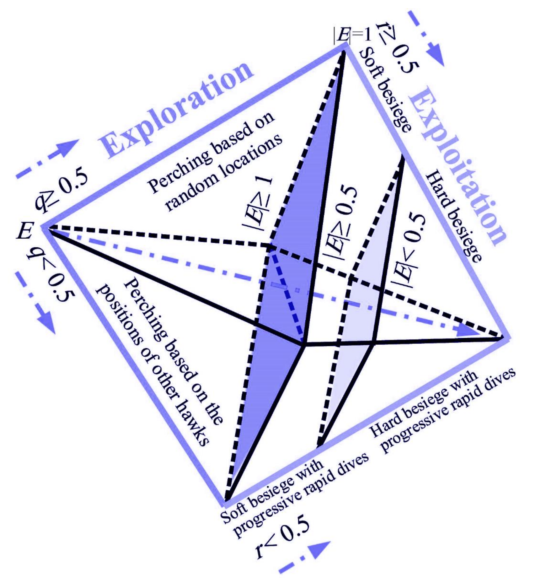
Recently, Heidari and his co-authors proposed a new nature-inspired meta-heuristic optimizer named Harris Hawks Optimization (HHO) [
20]. HHO simulates the behavior of hawks when they surprisingly attack their prey from different directions. HHO has several merits; it is simple, flexible, and free of internal parameters. Furthermore, it has a variety of exploitation and exploration strategies that ensure good results favorable convergence speed [
21]. The original real-valued version of the HHO algorithm has been applied in conjunction with various techniques to solve many optimization problems belonging to different domains [
22,
23,
24,
25,
26]. HHO has also been applied for solving FS problems [
27,
28,
29].
Broadly, several binarization schemes have been introduced to adapt real-valued meta-heuristics to deal with discrete search space. These approaches follow two major branches. The first branch is named continuous-binary operator, in which the meta-heuristic is adapted to work in binary search space by redefining the basic real values operators of its equations into binary operators [
30]. However, in the second branch, which is named two-step binarization, real values operators of meta-heuristics are kept without adjustment. To conduct the binarization, the first stage involves employing a transfer function (TF) to convert the real-valued solution R
into an intermediate probability vector [0, 1]
. Each element in the probability vector determines the probability of transforming its equivalent in R
into 0 or 1. In the second stage, a binarization rule is applied to transform the output of TF into a binary solution [
30]. In general, the second binarization scheme is commonly used for adapting meta-heuristics to work in binary search space. In this regard, Transfer Functions (TFs) are defined depending on their shapes into two types: S-shaped and V-shaped [
31,
32,
33]. Traditional or time-independent TFs are not able to deliver a satisfactory balance between exploration and exploitation in the search space. To overcome this shortcoming, several time-varying TFs have been proposed and applied with many meta-heuristic algorithms for providing a good balance between exploration and exploitation over iterations [
34,
35,
36].
In this work, to be utilized for FS tasks, the authors integrate time-varying versions of V-shaped TFs into the HHO algorithm to convert the continuous HHO into a binary version called BHHO. The benefit of using time-varying functions with the BHHO algorithm is to enhance its search ability by getting a better balance between exploration and exploitation phases. Time-varying functions also help in avoiding BHHO from getting stuck in local minima. The proposed approach is verified through eighteen benchmark datasets and revealed excellent performance compared to other state-of-the-art methods.
The rest of this article is organized as follows:
Section 2 introduces the related works, whereas
Section 3 presents the HHO algorithm.
Section 4 presents the proposed BHHO variants.
Section 5 outlines FS using the BHHO algorithm. Results and discussions are presented in
Section 6, while the conclusion in
Section 7 sums up the main findings of this work.
2. Related Works
The literature reveals that meta-heuristic algorithms have been very successful in tackling FS problems. GA and PSO algorithms have been utilized to develop effective FS methods for many problems. Several GA-based approaches have been proposed. Examples of these approaches are [
37,
38,
39,
40,
41]. Moreover, many binary variants of PSO have been frequently applied in many FS methods. Some examples can be found in Chuang et al. [
42], Chantar et al. [
4], Mafarja et al. [
43], and Moradi et al. [
44]. For instance, in Chuang et al. [
42], an improved version of Binary PSO named Chaotic BPSO was used for FS in which two chaotic maps called logistic and tent were embedded in BPSO for estimating the value of inertia weight in the velocity equation of PSO algorithm. Another example is the recent work of Mafarja et al. [
43], where five strategies were used to update the value of the inertia weight parameter during the search process. The proposed approaches have shown better performance when compared to other similar FS approaches. ACO algorithm, which was introduced by Dorigo et al. [
45] was also applied in FS. As examples, one can refer to the work of Deriche M. [
46], Chen et al. [
47], and Kashef et al. [
48]. Artificial Bee Colony (ABC) optimizer [
49]. An example of using the ABC algorithm for FS is presented in [
50]. In addition, as shown in [
51], the binary version of the well-known meta-heuristic Bat Algorithm (BA) was used as an FS method. Experiential results demonstrated the superiority of BA based FS method in contrast with GA and PSO-based methods. In addition to the algorithms mentioned above that have been applied for FS, many recently introduced meta-heuristic algorithms such as Slap Swarm Algorithm (SSA) [
6], Moth-Flame Optimization (MFO) [
52], Dragonfly Algorithm (DA) [
53], and Ant Lion Optimization (ALO) [
54] have been successfully utilized in FS for many classification problems.
Harris Hawks algorithm has been utilized to solve many optimization problems. For instance, as stated in [
23], in the civil engineering domain, HHO was used to improve the performance of the artificial neural network classifier in predicting the soil slope stability. In addition, a hybrid model based on HHO and Differential Evaluation (DE) algorithms has been applied to tackle the task of color image segmentation. Using different measures for evaluation purposes, results prove that HHO-DE based approach is superior compared to several state-of-the-arts image segmentation techniques [
24]. A novel automatic approach combining deep learning and optimization algorithms for nine control chart patterns (CCPs) recognition was proposed by [
25]. An HHO algorithm was applied for the best tuning of ConvNet parameters. In addition, an improved version of the HHO algorithm that incorporates three strategies, including chaos, topological multi-population, and differential evolution (DE), was proposed by [
26]. DE-driven multi-population HHO (CMDHHO) algorithm has shown its effectiveness in solving real-world optimization problems.
The investigated literature reveals that some binary versions of HHO have been proposed since the appearance of the HHO algorithm in 2019 for FS problems [
27,
28,
29,
55]. As presented in [
27], a set of binary variants of the HHO algorithm was proposed as wrapper FS methods. Eight V-shaped and S-shaped TFs and four quadratic functions were used to transform the search space from continuous to binary. The performance of proposed variants of BHHO are compared with binary forms of different optimization algorithms, include DE algorithm, binary Flower Pollination Algorithm (FPA), binary Multi-Verse Optimizer (MVO), binary SSA, and GA. The experimental results show that the QBHHO approach can mostly perform the best in terms of classification accuracy, least fitness value, and the lowest number of selected features. As stated in [
28], two binary variants of the HHO algorithm were proposed as wrapper FS approaches in which two transfer functions (S-shaped and V-shaped) were used to transform continuous search space into binary. Using several high dimension and low-sample challenging datasets along with different optimization algorithms (e.g., GA, BPSO, and BBA) for validating purposes, the S-shaped transfer function-based BHHO shows promising results in dealing with challenging datasets. Recently, Ref. [
55] proposed a wrapper-based FS for text classification in the Arabic context utilizing four binary variants of the HHO algorithm. The proposed variants of BHHO confirmed excellent performance compared to seven wrapper-based methods.
The traditional time-independent TFs are the most commonly used ones for adapting meta-heuristic algorithms to work in binary search space. For example, Kennedy and Eberhart [
31] used an S-shaped TF to convert PSO optimizer to deal with binary optimization problems. A V-shaped transfer function was adopted by [
33] to introduce a binary version of the Gravitational Search Algorithm (GSA). In 2013, for converting the continuous version of the PSO algorithm into Binary, Mirjalili and Lewis [
32] introduced six new V-shaped and S-shaped TFs for mapping continuous search space into a binary one. Experimental results approved that the new proposed V-shaped group of TFs can remarkably improve the performance of the classic version of PSO, especially in terms of convergence speed and avoiding local minima problems. In addition, the same set of TFs introduced by [
32] was also applied by Mafarja et al. [
56] to propose six versions of binary ALO. Results show that equipping ALO with V-shaped TFs can significantly improve its performance in terms of accuracy and preventing local minima.
Time-varying TFs were proposed by Islam et al. [
34] for boosting the performance of BPSO in which a modified form of BPSO called TV
-BPSO that adopts a time-varying transfer function was introduced to overcome the drawbacks of traditional TFs by providing a better balance between exploration and exploitation for the BPSO through its optimization process. In addition, Mafarja et al. [
35] was also applied several time-varying S-shaped and V-shaped TFs for improving the exploitation and exploration power of the Binary DA (BDA). The experimental results confirmed the superiority of time-varying S-shaped BDA approaches when compared to other tested approaches. Recently, Kahya et al. [
36] investigated the use of a time-varying transfer function with a binary WOA for FS. The results confirmed that BWOA-TV2 has consistency in FS. It also provides high accuracy of the classification with better convergence over conventional algorithms such as Binary Firefly Algorithm (BFA) and BPSO.
4. Proposed Binary HHO
In general, optimization algorithms are initially developed for solving problems in the continuous search space. The basic forms of these algorithms can not be directly applied to deal with binary and discrete optimization problems. In the binary optimization field, the search space can be viewed as a hypercube in which a search agent can adjust its position in the search space by changing the bits of its position vector from 1 to 0 or vise versa [
34,
35]. In the literature, depending on the shape of function, two basic forms of TFs known as S-shaped and V-shaped are proposed for adapting continuous search into binary. The first S-shaped TF was proposed by Kennedy and Eberhart [
31] to transform the continuous original version of the PSO algorithm into a discrete one while the initial V-shaped transfer function was proposed by Rashedi et al. [
33] for developing a binary variant of GSA (BGSA). Although the sigmoid TF is simple, effective, cheap in terms of computational cost, and widely utilized for binary variants of optimization algorithms, it has some shortcomings. It is unable to provide sufficient balance between the two essential stages of the optimization process (exploration and exploitation). In addition, it also has difficulty in avoiding the stuck of the algorithm in local minima and controlling the convergence speed [
32]. In the case of V-shaped TF, it is defined based on some principles to map continuous values of velocity vectors into probabilities. The main concept is that the search agents that have significant absolute values of velocity are potentially far from the optimal solution; hence the TF should provide a high probability for changing the positions of search agents. When the velocity vector has small absolute values, then the TF should present small probability values of changing the positions of the search agents [
33].
To overcome the limitations of basic TFs in mapping velocity values to probability ones, Mirjalili and Lewis [
32] extensively studied the influence of the available TFs on the performance of BPSO. Accordingly, six new transfer functions divided into two groups according to their forms, S-shaped and V-shaped, were introduced for mapping the continuous search to discrete search space. It was found that V-shaped family of TFs, in particular V4 TF, significantly improves the performance of binary algorithms compared to the sigmoid TF. Furthermore, the same families of TFs were employed by Mafarja et al. in [
56] to develop six discrete forms of ALO for FS. It was observed that the V-shaped TFs, especially ALO-V3, significantly enhance the performance of binary ALO optimizer for FS tasks.
Following the appearance of various forms of TFs for adapting the optimization algorithms to work in discrete search space, in 2017, Islam et al. [
34] studied and analyzed the behavior and performance of existing TFs with the PSO algorithm in dealing with low and high dimensional discrete optimization problems. It was demonstrated that current TFs still suffer from difficulty in controlling the balance between exploration and exploitation of the optimization process. As presented in [
34], to overcome the limitations of current basic TFs, the authors defined some concepts in which the search process for an optimal solution should concentrate on the exploration in the early generations of the optimization process by letting the TF produce a high probability of changing the elements of the position vector of a search agent based on the value of the velocity vector (step). In later phases, the optimization process should move the focus of the search from exploration to exploitation by enabling the TF to provide a low probability of changing the position’s elements of a search agent. According to these concepts, a control parameter (
) was adopted in the TF, where this parameter starts with a large value and decreases gradually over the iteration to obtain a smooth shift from exploration to exploitation. In this way, the shape of the TF changes over time based on the value of the controlling parameter. The purpose of employing the time-varying scheme is to obtain a better balance between exploration and exploitation through the optimization process of a BPSO. Time-varying TFs demonstrated their superiority when compared to existing static TFs based on BPSO approaches over low-dimensional and high-dimensional discrete optimization problems.
Inspired by the work of [
32,
34], Mafarja et al. [
35] proposed eight time-varying TFs related into two families (S-shaped and V-shaped) for developing binary versions of DA (BDA) to be used for FS. The authors demonstrated the efficiency of these time-varying TFs by comparing their performance with other static TFs as well as various wrapper-based FS approaches. In addition, three types of time-varying transfer functions were introduced in [
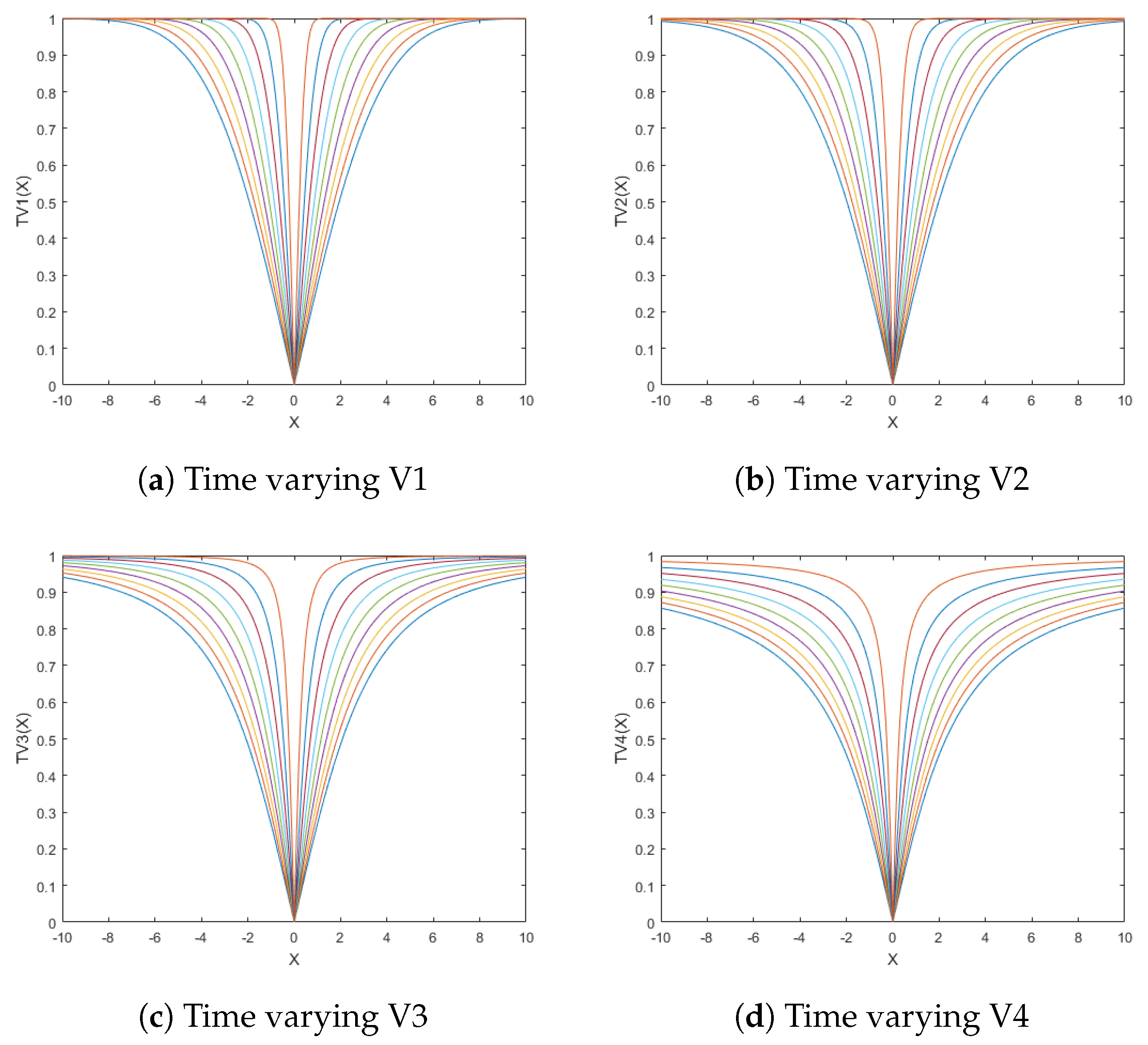
36] for improving the performance of the binary WOA in the FS domain. WOA with time-varying TFs has shown higher effectiveness and efficiency than other popular approaches in the FS domain. In this work, considering the previous studies of the impact of TFs on the performance of binary optimization algorithms, we select the time-varying TFs, specifically V-shaped, proposed by [
35], as shown in
Table 1, to convert HHO to binary and apply the binary variants of HHO to the FS problem. In the time-varying form of the TFs,
represents a time-varying variable that begins with an initial value and progressively reduces over iterations, as shown in Equation (
14).
where
and
represent the bounds of the
parameter,
t denotes the current iteration, and
T represents the maximum number of iterations. In this study,
and
were selected to be 0.01 and 4, respectively [
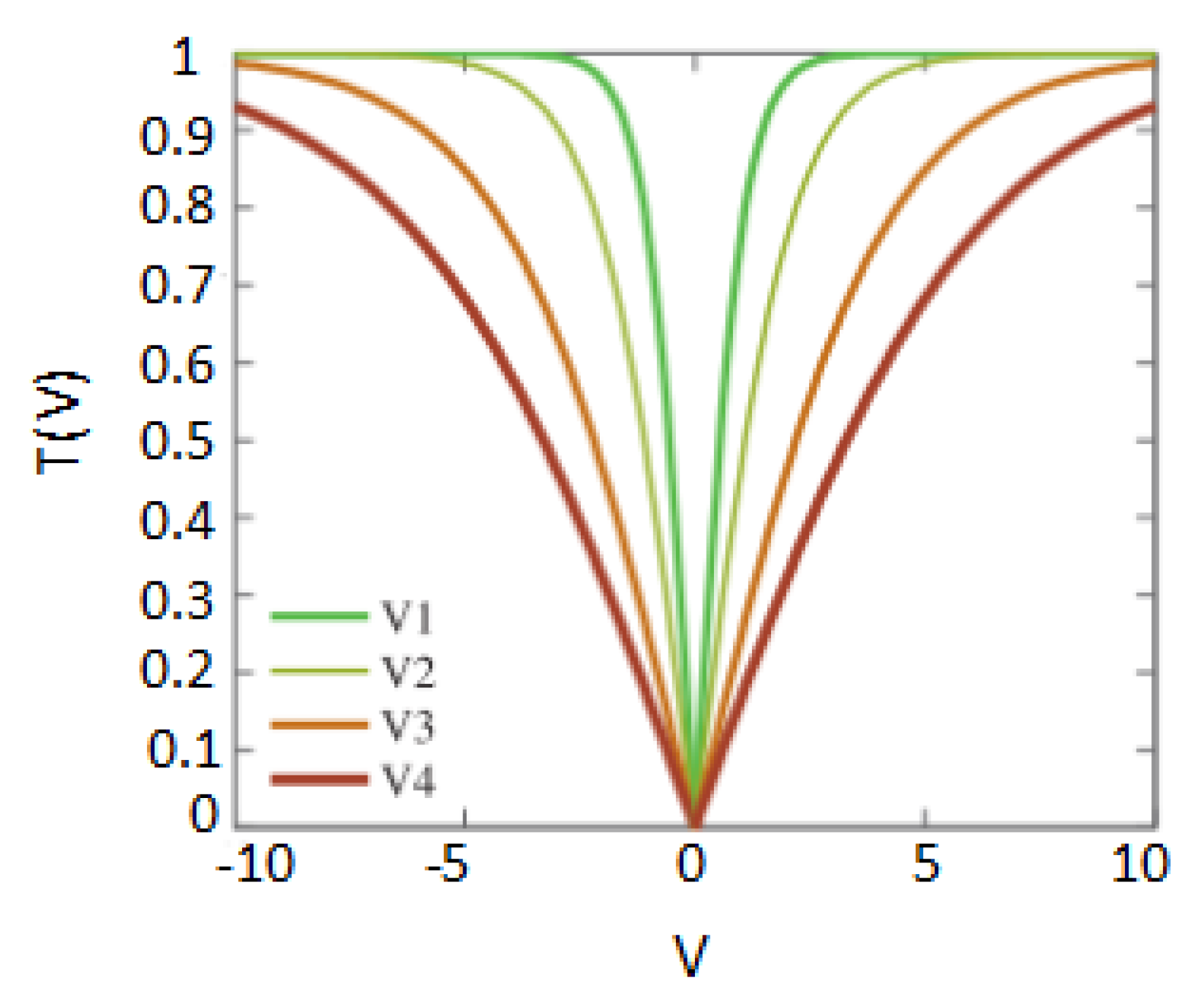
35]. The original time independent V-shaped TFs are shown in
Figure 2, while the time varying variants of TFs are shown in
Figure 3.
After employing the original or time-varying TFs as a first step in the binarization scheme, the real-valued solution R
is converted into an intermediate probability vector [0, 1]
such that each of its element determines the probability of transforming its equivalent in R
into 0 or 1. In the second step, a binarization rule is applied to transform the output of TFs into a binary solution [
30]. In this work, the complement binarization introduced by Rashedi et al. [
33] is applied as given in Equation (
15).
where ∽ denotes the complement,
is the current binary value for the
jth element, and
is the new binary value. It is noted that the updated binary value is set considering the current binary solution, that is, based on the probability value
, the
jth element is either kept or flipped.
Algorithm 1 explains the pseudo-code of the Binary HHO algorithm.
| Algorithm 1 Pseudo-code of the BHHO algorithm. |
Inputs: Number of hawks (N) and maximum iterations (T) Outputs: Generate the initial binary population while (t < T) do Evaluate the fitness values of hawks Find out the best search agent for (each hawk ()) do Update and jump strength J ▹E=2rand()−1, J=2(1−rand()) if () then ▹ Exploration phase Update the position vector by Equation ( 1) Calculate the probability vector using time-varying V-shaped TFs Calculate the binary solution using Equation ( 15) if () then ▹ Exploitation phase if (0.5) then if ( ) then ▹ Soft besiege Update the position vector by Equation ( 4) else if ( ) then ▹ Hard besiege Update the position vector by Equation ( 6) Calculate the probability vector using time-varying V-shaped TFs Calculate the binary solution using Equation ( 15) if (0.5) then if ( ) then ▹ Soft besiege with progressive rapid dives Calculate Y and Z using Equations ( 7) and ( 8) Convert Y and Z into binary using time-varying TF and binarization rule in Equation ( 15) Update the position vector by Equation ( 10) else if ( ) then ▹ Hard besiege with progressive rapid dives Calculate Y’ and Z’ using Equations ( 12) and ( 13) Convert Y’ and Z’ into binary using time-varying TF and binarization rule in Equation ( 15) Update the position vector by Equation ( 11) Return
|
6. Results and Discussion
In this section, we have conducted various experiments and tests to assess the performance of V-shaped time-varying-based HHO algorithms in solving the FS problem. The proposed BHHO algorithms were also compared to different optimizers. To achieve a fair comparison, the initial settings of all optimizers, such as population size, number of iterations, and number of independent runs, were unified by setting them to similar initials values.
Eighteen popular benchmark datasets obtained from the UCI data repository are applied for evaluating the performance of the proposed FS approaches.
Table 2 shows the details of the datasets comprising a number of features, classes, and instances in each dataset. Following the hold-out method, each dataset is arbitrarily split into two portions (training/testing), where 80% of the data were preserved for training while the rest was employed for testing. Furthermore, each FS approach was run for 30 trials with a randomly set seed on a machine with an Intel Core i5, 2.2 GHz CPU, and 4 GB of RAM.
In this work, internal parameters of algorithms were set according to recommended settings in original papers as well as related works on FS problems, while common parameters were set based on the results of several trials.
Table 3 reveals the detailed parameters settings of each algorithm.
To study the impact of four types of time-varying V-shaped TFs on the efficiency of the BHHO optimizer, we provide comparisons between the results of HHO with four basic V-shaped TFs and those recorded by HHO with four time-varying V-shaped TFs. Furthermore, the best FS approach among tested basic and time-varying V-shaped based approaches was then compared to several state-of-the-art FS approaches comprising BGSA, BPSO, BBA, BSSA, and BWOA. The following criteria were used for the comparisons:
The average of accuracy rates obtained from 30 trials.
The average of best selected features rates recorded from 30 trials.
The mean of best fitness values obtained from 30 trials.
F-test method is used for ranking different FS methods to determine the best results.
Please note that in all reported tables, the best-obtained results are highlighted using a boldface format.
6.1. Comparison between Various Versions of BHHO with Basic and Time Varying V-Shaped TFs
In general, experimental results show that HHO with V-shaped time-varying transfer functions (TV-TFs) is better compared to those with classic V-shaped TFs. Inspecting the results in
Table 4, in the case of BHHO
and BHHO
, BHHO
has recorded higher accuracy rates on seven datasets while BHHO
has found higher accuracy rates for eight cases. However, both approaches have the same accuracy rates in three cases. In addition, we see that BHHO
has better accuracy measures than BHHO
on eleven datasets, whereas BHHO
outperforms BHHO
in five cases. It can be observed that BHHO
and BHHO
have maximum accuracy rates in two cases (M-of-N and Zoo). In the case of BHHO
and BHHO
, it can be noticed that BHHO
outperforms BHHO
on nine datasets while BHHO
obtained higher accuracy rates on five datasets. It can be seen that both approaches obtained similar accuracy rates on the exactly dataset and the maximum accuracy measures on three datasets, including M-of-N, WineEW, and Zoo. As per results, BHHO
outperforms BHHO
on eleven datasets in terms of accuracy rates, whereas BHHO
is superior in only three cases. However, both methods obtained similar maximum obtained maximum accuracy rates on four datasets. In terms of classification accuracy, as per F-test results, it can be seen that BHHO
is ranked as the best, followed by the BHHO
method. Based on the observed results, we can say that HHO with TV4 transfer function is able to obtain the best classification accuracy compared to its peers, including basic and time-varying TFs-based FS approaches.
In terms of selected features, as presented in
Table 5, it can be seen that the basic versions of V1 and V2 based approaches outperform the time-varying-based ones. In the case of BHHO
and BHHO
, it is clear that BHHO
is dominant on 61.11% of cases while BHHO
outperformed BHHO
on 50% of the cases. According to recorded FS rates, F-test results show that BHHO
is ranked as the best method in terms of the least number of selected features. However, excessive feature reduction may not be the preferred option since it may exclude some relevant features, which degrade the classification performance. Although the basic versions of TFs-based approaches outperform the time-varying-based ones in terms of feature reduction, the latter can find the most relevant subset of features that provides better classification accuracy, as provided in
Table 4.
To confirm the effectiveness of the competing algorithms, the fitness value that combines the two measures (i.e., accuracy and reduction rate) is adopted. In terms of fitness rates, as provided in
Table 6, it is clear that all time-varying V-shaped TFs based methods outperform their peers (basic V-shaped-based techniques) in terms of fitness rates. Considering F-test results, BHHO
is ranked as the best place compared to all other competitors. In this work, we consider that classification accuracy has higher importance compared to the number of selected features. Based on results, we found that HHO with time-varying V-shaped TV4 can realize the best performance.
6.2. Comparison with Other Optimization Algorithms
This section provides a comparison between the best approach BHHO and other well-known metaheuristic methods (BGSA, BPSO, BBA, BSSA, and BWOA). The comparison is made based on different criteria, including average classification accuracy, number of selected features, and fitness values.
As per results in
Table 7, it can be observed that BHHO
outperforms other algorithms for 11 out of 18 datasets in terms of accuracy rates. It reached the maximum accuracy averages on five datasets. We see that BHHO
, BPSO, and BSSA reached maximum accuracy for the Zoo dataset. In addition, compared to BHHO
, it can be seen that BPSO obtained better results on Exactly2, Vote, and WaveformEW datasets. As per F-test results, we observe the BHHO
is ranked one, followed by BPSO, BSSA, BWOA, BGSA, and BBA methods. To see whether the differences between obtained results from BHHO
and other algorithms are statistically significant or not, a two-tailed Wilcoxon statistical test with 5% significance was used.
Table 8 presents the p-values of the Wilcoxon test in terms of classification accuracy. It is clear that there are meaningful differences in terms of accuracy averages between BHHO
and its competitors in most of the cases.
In terms of the least number of selected features, as stated in
Table 9, it is observed that BHHO
obtained the best averages on 13 out of 18 datasets while BPSO outperforms all other algorithms on three datasets. As per F-test results, we can see that the BHHO
is ranked as the best one, followed by BPSO, and BBA methods, respectively. Inspecting the results of the
p-value in
Table 10, it is evident that the insignificant differences in terms of the lowest number of selected features between BHHO
and other peers are limited.
Fitness rates are shown in
Table 11, and it can be noticed that BHHO
reached the lowest fitness values compared with other algorithms on 11 out of 18 datasets. We can also see that BPSO is the best in four cases. Again, according to F-test results as in
Table 11, it is clear that the BHHO
is ranked as the best, followed by the BPSO method. In addition,
Table 12 shows the
p-values of the Wilcoxon test in terms of best fitness rates. It can be observed that the differences between BHHO
and others are not statistically significant in only four cases.
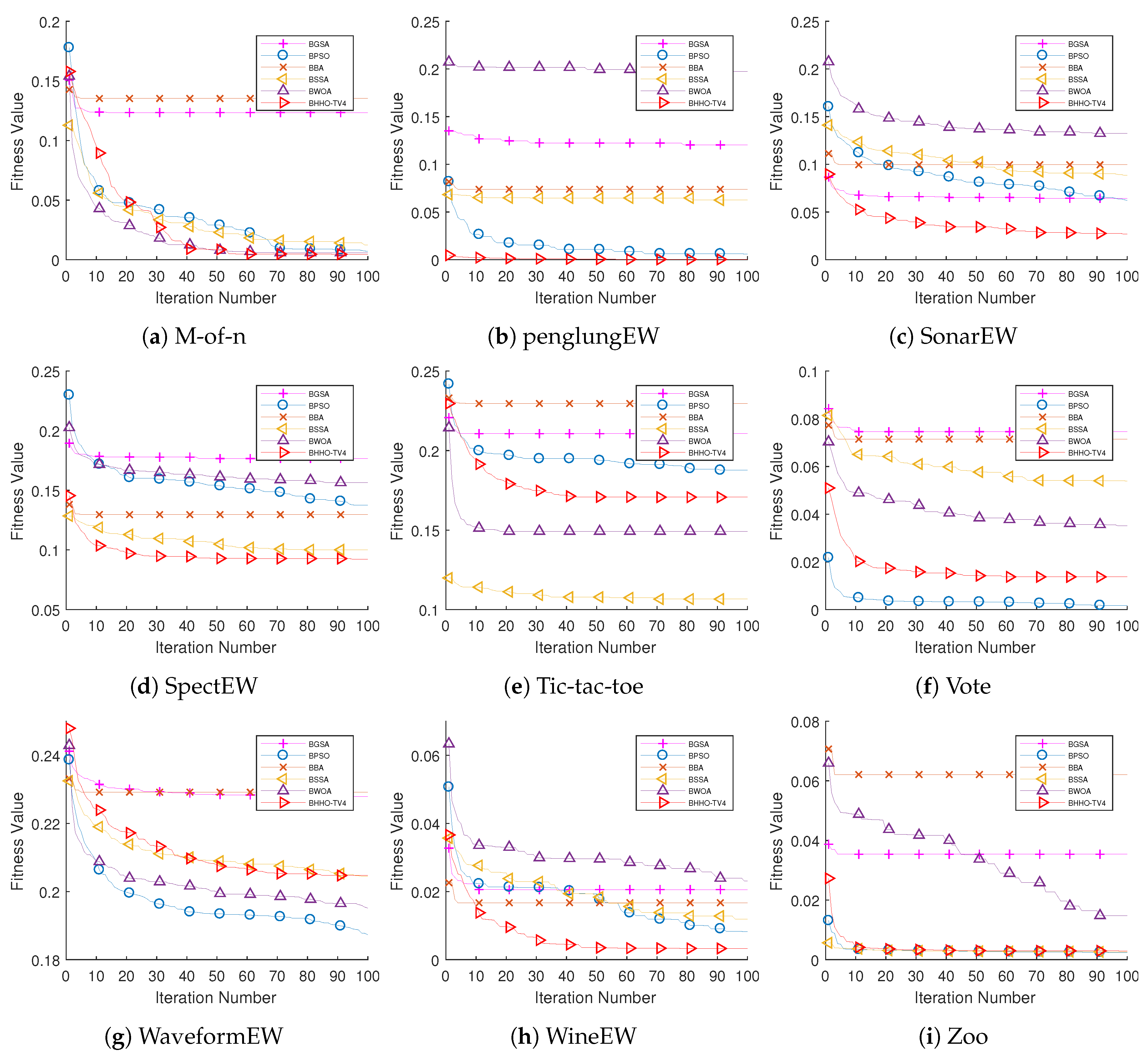
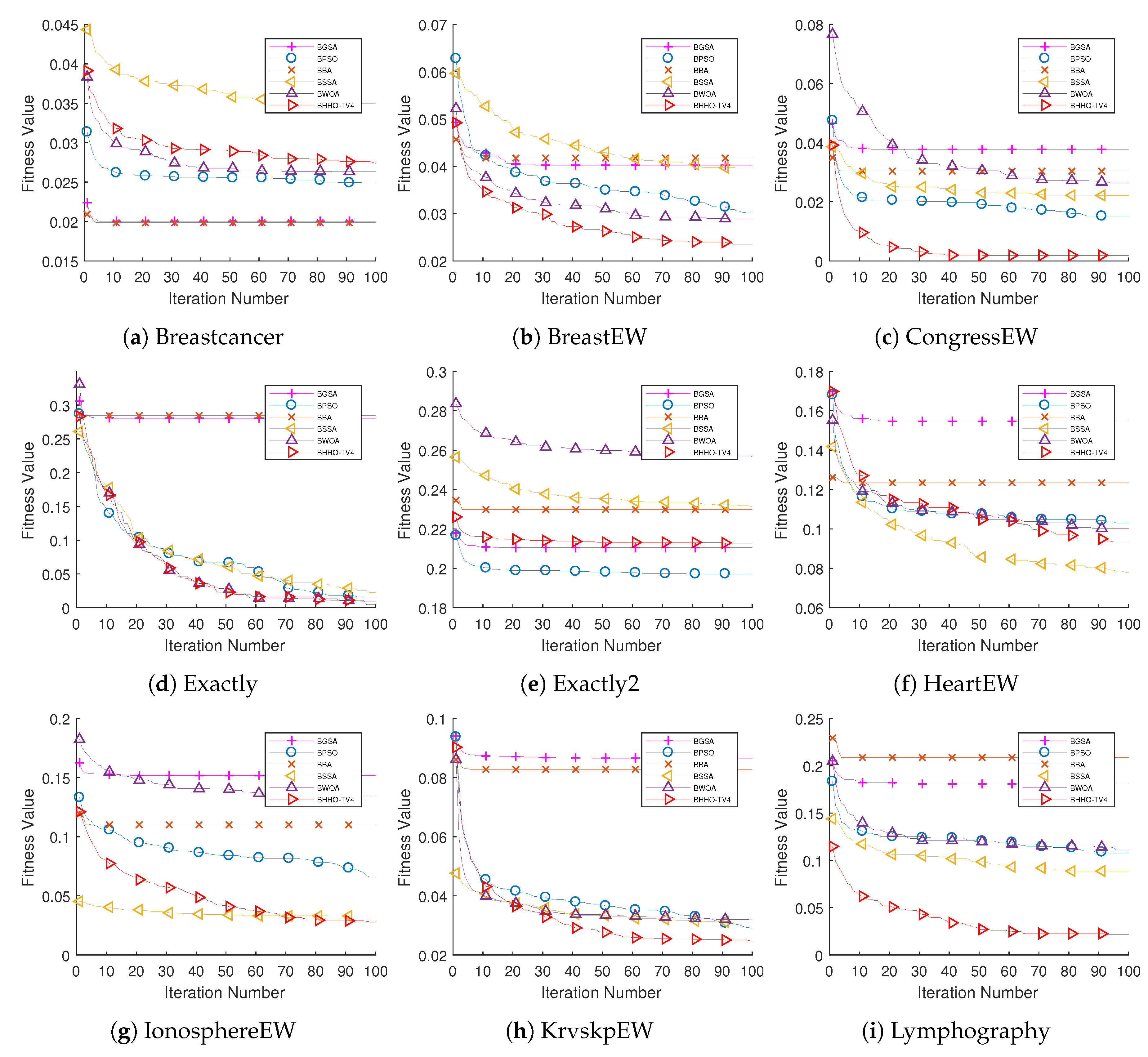
The convergence behaviors of BHHO
and other algorithms were also investigated to assess their ability to make an adequate balance between exploration and exploitation by avoiding local optima and early convergence. The convergence behaviors of BHHO
on 12 datasets compared to other optimizers are demonstrated in
Figure 4 and
Figure 5. In all tested cases, the superiority of BHHO
can be seen in converging faster than other competitors towards the optimal solution.
6.3. Comparison with Results of Previous Works
This section provides comparisons of accuracy rates between optimal approach BHHO
in this research and its similar FS approaches introduced in previous studies. Results of BHHO
are compared with results of SSA in [
58], WOA in [
59], Grasshopper Optimization Algorithm (GOA) in [
60], GSA boosted with evolutionary crossover and mutation operators in [
61], GOA with Evolutionary Population Dynamics (EPD) stochastic search strategies in [
62], BDA [
35], hybrid approach based on Grey Wolf Optimization (GWO) and PSO in [
12] and Binary Butterfly Optimization Algorithm (BOA) [
63]. As in
Table 13, it can be seen that the proposed approach BHHO
has achieved the best accuracy rates on twelve datasets compared to results presented in previous studies on the same datasets. We can also observe that BHHO
reached the highest accuracy rates on six datasets. In addition, the F-test results indicate that BHHO
is ranked as the best in comparison with results of other algorithms used in preceding works.
In general, the results reflect the impact of the adopted binarization scheme on the performance of HHO in scanning the binary search space for finding the optimal solution (e.g., the ideal or near to the ideal subset of features). It is evident that the utilized time-varying TFs, in particular, TV can remarkably enhance the exploration and exploitation of the HHO algorithm. A potential key factor behind the superiority of BHHO is that changing the shape of TV transfer function over generations has enabled the HHO algorithm to obtain an appropriate balance between exploration and exploitation phases and boosted the HHO algorithm to reach areas containing highly valuable features in the search space. Furthermore, similar to many materialistic algorithms, HHO suffers from the problem of sliding into local optima. The accuracy rates of BHHO compared to other algorithms prove its superior capability in preserving the population diversity during the search procedure. Hence, preventing the occurrence of an early convergence problem.


