Feed-Forward Neural Networks for Failure Mechanics Problems

Abstract

This work addresses an efficient neural network (NN) representation for the phase-field modeling of isotropic brittle fracture. In recent years, data-driven approaches, such as neural networks, have become an active research field in mechanics. In this contribution, deep neural networks—in particular, the feed-forward neural network (FFNN)—are utilized directly for the development of the failure model. The verification and generalization of the trained models for elasticity as well as fracture behavior are investigated by several representative numerical examples under different loading conditions. As an outcome, promising results close to the exact solutions are produced.

1. Introduction

Various discretization schemes exist in the literature for solving different science and engineering problems, e.g., the finite element method (FEM) [1], isogeometric analysis (IGA) [2], and the virtual element method (VEM) [3]. These modern element technologies heavily depend on the availability of a “material model” that describes the nonlinear behavior of the material as well as the structural failure. Such analytical and physically motivated mathematical models lead to a pronounced computational cost. Thus, a computationally less expensive approach has always been sought after. In this regard, one of the current possibilities introduced in the literature is the employment of unconventional approaches, such as data-driven models, to reduce the computation costs [4,5,6,7,8,9]. Machine learning, deep learning, and neural networks are examples of such data-driven models that help to reduce model complexity and may surpass conventional constitutive modeling [4,7,8,10,11].

Hitherto, a great number of machine learning motivated applications for modeling the constitutive behavior of materials has been published in the literature; see [12,13,14,15,16,17,18,19] and the citation therein.

1.1. Motivation and State of the Art

The inspiration for implementing machine learning approaches, more specifically, artificial neural networks (ANNs), to a wide range of engineering disciplines comes from human and animal neural systems. These biologically inspired simulations, performed on the computer, carry out many tasks, e.g., clustering, classification, and pattern recognition. Recently, ANNs were satisfyingly used in voice/image recognition and robotics. In the field of mechanics, novel investigations have been proposed in the literature. To this end, the so-called self-learning finite element procedure introduced by Ghaboussi et al. [20] and developed by Shin and Pande [21] can be mentioned as a very auspicious technique for the ANNs training process. Further interesting reviews of possible applications of ANNs in mechanics can be seen in [22,23,24], and their application for constitutive modeling in [25,26].

To incorporate data-driven models for solving computational mechanics problems by taking over classical constitutive modeling, numerous approaches have been proposed in the literature. This contribution represents the first steps toward deep learning (DL) as a subset of machine learning that extracts patterns from data, using neural networks for inelastic solids.

1.2. Deep Learning (DL) Architectures

DL has many architectures, especially in mechanics, and research is focused mainly on using the feed-forward neural network (FFNN), recurrent neural network (RNN), and convolutional neural network (CNN). So far, applications of these types of neural networks devoted to the field of mechanics can be seen in the recent works of [27,28,29,30,31,32,33,34,35,36,37,38,39,40,41,42,43]. A detailed description of those approaches is summarized as follows:

• FFNN is used in [44,45] to model the material behavior at the macroscale level, using strains (as inputs) and stresses (as outputs). One main advantage of such a model is that the training data required for the neural network can be directly acquired from experimental data. On this basis, and for modeling a neural network that approximates the non-linear behavior of history-dependent material models (e.g., plasticity, where loading history is relevant), Ref. [46] proposed the incorporation of the strain from the previous load step as an input data or feature for the neural network. Recently, a novel method called the proper orthogonal decomposition feed forward neural network (PODFNN) was proposed by [47] for predicting the stress sequences in the case of plasticity, which reduces the complexity of the model significantly by transforming the stress sequence into multiple independent coefficient sequences.
• RNN is another type of neural network that uses the previous outputs as inputs, i.e., path-dependent scheme. Two different approaches, direct (black box) and graph-based (physically-informed), were applied in [37] for modeling elastoplastic materials. In the former case (black box approach), the total stress was predicted purely considering the total strain history, whereas in the latter case (graph-based approach), besides using the recurrent neural network to predict the path-dependent behavior, the feed forward neural network is used to predict the path-independent responses, which may lead to a more accurate prediction of stresses.
• CNN is a special type of deep neural network that has recently become a dominant method in computer vision. A CNN architecture consists of an input and an output layer, as well as multiple hidden layers. These hidden layers typically consist of convolutional layers, activation layers, pooling layers, and fully connected layers. CNNs have been used in image classification, video classification, face recognition, scene labeling, action recognition, image segmentation, and natural language translation, among others. In the work of [48] CNNs are used to quantitatively predict the mechanical properties (i.e., stiffness, strength, and toughness) of a 2D checkerboard composed of two different phases (brittle and ductile). Following this line, Ref. [49] introduced a graph convolutional deep neural network, incorporating the non-Euclidean weighted graph data to predict the elastic response of materials with complex microstructures. For recent works on CNNs, we refer to [50,51,52], and the citations therein.

Within this work, a feed-forward neural network (FFNN) is employed to perform the regression task of predicting stresses in the case of linear elastic material and also predicting the elasticity in the fracture phase-field modeling of brittle solids along with the prediction of the crack phase field. The objective of this paper is to incorporate neural network models as constitutive models within the finite element applications for elasticity and phase-field modeling of brittle fracture by combining the available tools. The efficiency of the trained neural network is studied within the finite element analysis. The raw numerical data acquired by FEM simulation are used to train the neural network model under investigation. As an advantage of this contribution, the proposed method has the potential for providing accurate and feasible approximations for various engineering applications. To this end, promising results close to the exact solution are achieved, provided that the training data set contains all the possible patterns as the target problem. Note that this paper represents an initial contribution to the use of neural networks for solving fracture mechanics problems. Hence, as a starting point, the model performance is evaluated through numerical results instead of real experimental data.

The paper is organized as follows: In Section 2 a brief overview of the neural network, in particular the feed-forward neural network, for path-independent predictions is presented. In Section 3, the trained network is applied to learn the constitutive behavior of elastic materials within the finite element application. Then, the trained model is used to predict the elasticity in the phase-field fracture simulation in Section 4. Thereafter, the data collection strategy for predicting phase-field fracture using a neural network model is developed and validated in Section 5. Section 6 presents a summary and the outlook of this work.

2. Theory of Neural Networks

A neural network (NN) algorithm can be described using a data set, a model, a loss-function, and an optimization procedure. A data set refers to the total samples available for the training, validation, and testing of an algorithm. It is commonly split into three parts: training, validation, and test sets. The algorithm learns from the training set. Then, a validation set is used to evaluate and optimize the learning algorithm. Finally, the testing set acts as unseen data, and is used to test the trained algorithm. A model refers to the structure that holds all information that describes the (learned function) trained algorithm. A loss function or objective function is a metric that must be minimized during training. The optimization procedure is used to find the optimal parameters of the model that minimizes the loss function. A more detailed analysis of neural networks can be found, for instance in [53].

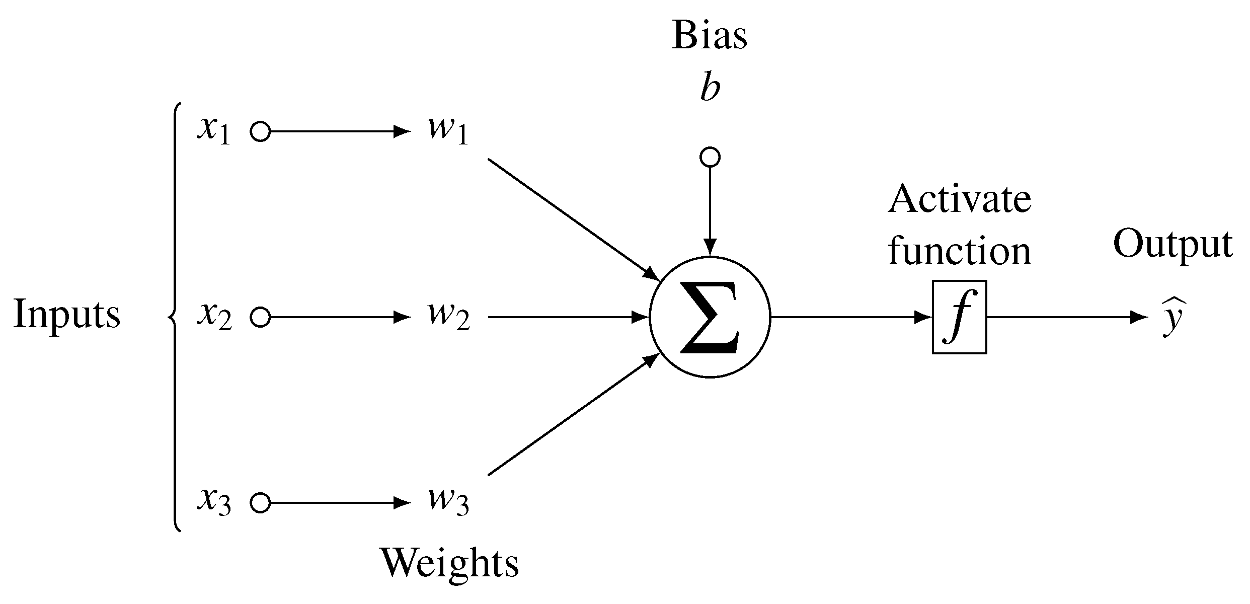
2.1. Artificial Neural Network (ANN)

ANN is defined as a mathematical model divided into a series of interconnected elements classified in layers, whose geometry and functionality have been compared with those of the human brain. ANN is made up of neurons that have one scalar output and multiple inputs, as sketched in Figure 1.

An inventive but simple structure is composed of four parts: (i) input values, (ii) weights and bias, (iii) weighted total (sum), and (iv) activation function (threshold unit). A schematic diagram of an artificial neuron is illustrated in Figure 1, where, $x_1-x_3$ are inputs, $w_1-w_3$ are their corresponding weights, b is the bias, f is the activation function applied to the weighted sum of the inputs and $\widehat{y}$ is the output of the neuron.

Mathematically, this relation can be written as follows:

$$\widehat{y}=f(\sum _{i=1}^N{\mathit{x}}_{\mathit{i}}{\mathit{w}}_{\mathit{i}}+b),$$

(1)

where N is the number of samples. Equation (1) can be rewritten in the following compact form as follows:

$$\widehat{y}=f({\mathit{x}}^{\mathit{T}}\mathit{W}+b) \mathrm{with} \mathit{x}={[x_1,\dots ,x_N]}^T \mathrm{and} \mathit{W}={[w_1,\dots ,w_N]}^T.$$

(2)

The activation function f (also known as the transfer function) determines the output of neurons in the neural network model, its computational efficiency and its ability to train and converge after multiple iterations of training. This introduces non-linear properties to the network. Hence, its main purpose is to convert the input signal of a node in an ANN to an output signal. The output signal is then used as an input in the next layer of the neural network.

Specifically, in ANN, a sum of products is performed for inputs x and the corresponding weights W. Next, the activation function $f\left(x\right)$ is applied to obtain the output of that layer and feed it as an input to the next layer. Activation functions can be linear and non-linear. A linear activation function (e.g., Purelin activation function) contains an infinite range and has no effect on the complexity of the data set. On the other hand, non-linear activation functions (e.g., Sigmoid and Tanh activation functions) introduce non-linearity in order to better learn the complex relationship between the input and output data. Here, the most widely used classic activation functions with their first derivatives are presented as follows:

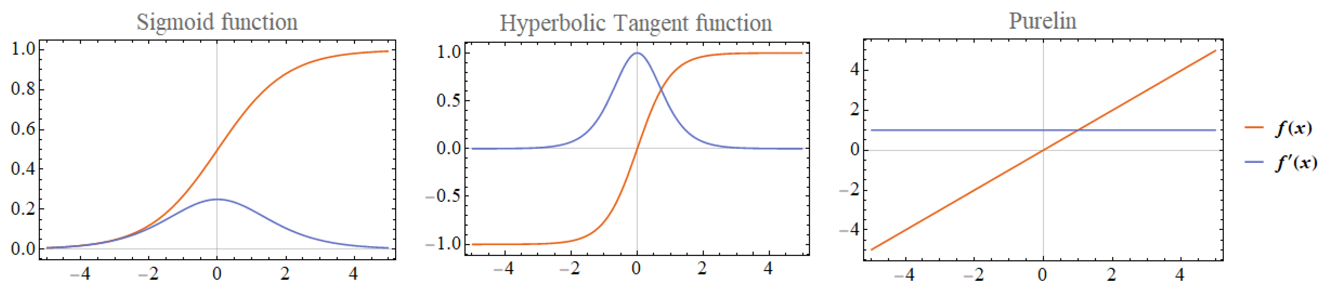
• Sigmoid transfer function.

  $$f\left(x\right)=\frac{1}{e^{-x}+1};f^{\prime }\left(x\right)=\frac{e^{-x}}{{\left(e^{-x}+1\right)}^2}$$

  (3)
• Hyperbolic tangent (Tan–Sigmoid transfer function).

  $$f\left(x\right)=\frac{e^x-e^{-x}}{e^x+e^{-x}};f^{\prime }\left(x\right)=1-\frac{{\left(e^x-e^{-x}\right)}^2}{{\left(e^{-x}+e^x\right)}^2}=4\frac{e^{2x}}{{(1+e^{2x})}^2}$$

  (4)
• Purelin function.

  $$f\left(x\right)=x;f^{\prime }\left(x\right)=1$$

  (5)

  Figure 2 illustrates those functions and their derivatives.

A key aspect of the activation function is that it should be differentiable for performing a successful backpropagation optimization strategy. In this paper, we used the hyperbolic tangent function, due to its flexible range and general applicability in different engineering problems; see, for example, [53].

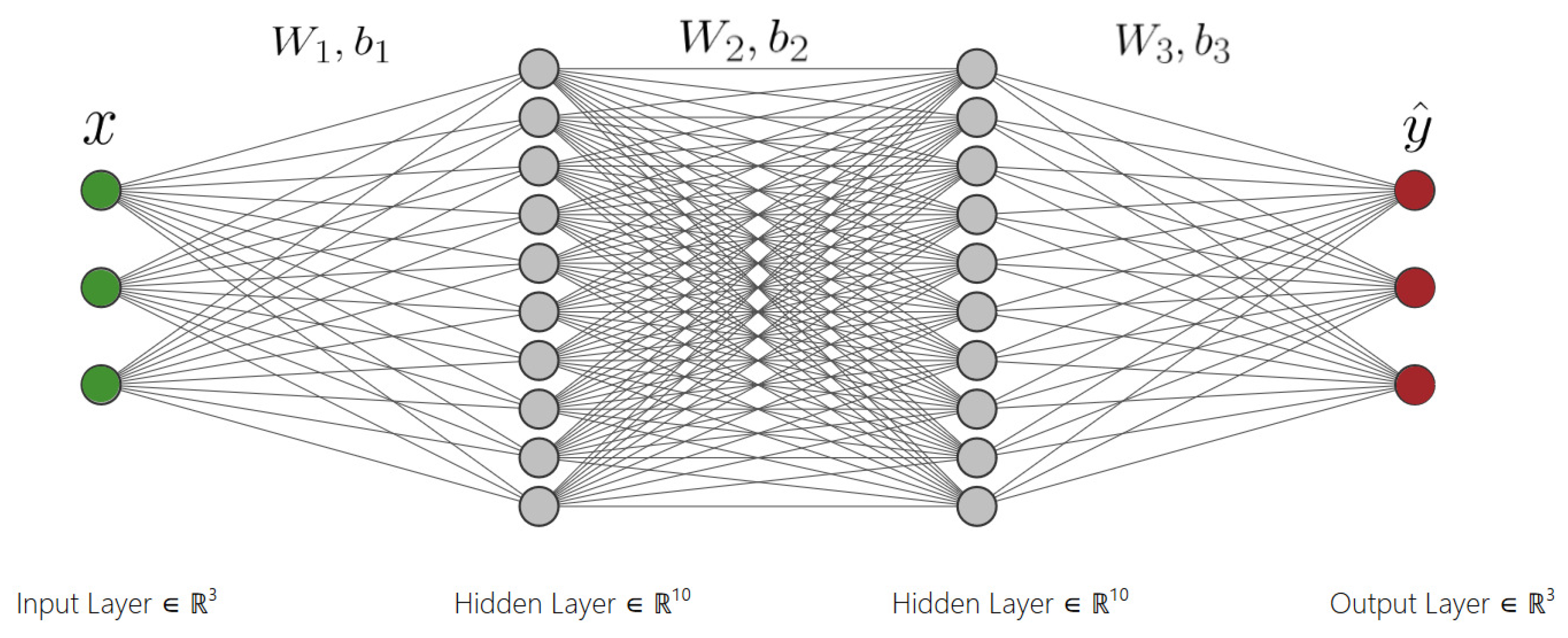
2.2. Feed-Forward Neural Network (FFNN)

In a FFNN, the number of inputs and outputs are fixed and the knowledge of history variables is disregarded. According to the complexity of the training data, the architecture of the FFNN (to be more specific, the number of hidden layers and neurons in each layer) has to be determined. In this paper, Machine Learning Toolbox (nntraintool) is used to train the model under consideration (nntraintool is a Matlab toolbox that is used for training neural networks. It is divided into four parts, such as the neural network architecture, algorithms, training progress, and plots. Interested readers are referred to [Neural network training tool—MATLAB nntraintool (mathworks.com accessed on 7 July 2021)]).

The formulation of a fully-connected feed forward neural network with two hidden layers $\mathit{H}$, shown in Figure 3, is defined as follows:

$$\widehat{\mathit{y}}=f({\mathit{H}}_2{\mathit{W}}_3+{\mathit{b}}_3) \mathrm{with} {\mathit{H}}_2=f({\mathit{H}}_1{\mathit{W}}_2+{\mathit{b}}_2) \mathrm{and} {\mathit{H}}_1=f({\mathit{xW}}_1+{\mathit{b}}_1),$$

(6)

where the vector $\widehat{\mathit{y}}$ is the output, the input vector x contains the features of a sample, W is the weight matrix, and b is the bias vector for each respective layer. In the current study, hidden layers have the tangent hyperbolic activation function f, which is formulated as follows:

$$tanh\left(x\right)=\frac{e^x-e^{-x}}{e^x+e^{-x}}.$$

(7)

This function is a rescaling of the logistic Sigmoid function, depicted in Figure 2, with an output range of $[-1,1]$. The hidden layers values are included in the vector $\mathit{H}$. The feed forward neural network architecture can be simplified as follows, given that $\mathit{y}$ is the true function:

$$\widehat{\mathit{y}}=\widehat{\mathit{y}}(\mathit{x},\mathit{W},\mathit{b}) \mathrm{and} \left\{{\mathit{b}}^{\prime },{\mathit{W}}^{\prime }\right\}=\mathrm{Arg}\left\{\underset{\mathit{b},\mathit{W}}{\min }\mathcal{L}\left(\widehat{\mathit{y}},\mathit{y}\right)\right\},$$

(8)

where the loss function $\mathcal{L}$ is minimized to find the optimized weights ${\mathit{W}}^{\prime }$ and biases ${\mathit{b}}^{\prime }$ of the trained neural network model. In this analysis, a feed forward neural network with two hidden layers (we have tried different architectures with hidden layers of different sizes; however, the final result was not affected. Therefore, for simplicity, we have kept the neural network architecture with two hidden layers throughout this research) of 10 neurons each is created such that strains ε are features and stresses σ are the outputs of the model.

Mean-squared error (MSE) is considered the loss function $\mathcal{L}$ such that it is minimized during the training process as follows:

$$MSE=\frac{1}{N}\sum _{i=1}^N{\left[{\left(x_{target}\right)}_i-{\left(x_{pred}\right)}_i\right]}^2.$$

(9)

Since the stress and strain values are on different scales of magnitude, it is important to scale the data set to a comparable range; therefore, the input and target data are initially scaled to be in the range $[-1,1]$ by using the following formula:

$$\overline{x}=\frac{2(x-x_{min})}{x_{max}-x_{min}}+1,$$

(10)

where $\overline{x}$ is the scaled or normalized value of x in the range of $[-1,1]$.

2.3. Neural Network Training

Training a neural network model is like solving an optimization problem, where the weights within the model are optimized such that it gets constantly updated during training. This procedure continues until their optimal values are reached. Hence, the optimization of weights depends on the optimization algorithm or optimizer that one chooses for modeling. In the presented contribution, Levenberg–Marquardt optimization [54] is employed, due to its memory efficiency. Furthermore, it is the fastest backpropagation algorithm which updates the weights and biases in the following Newton-like update:

$${\mathit{W}}^{n+1}={\mathit{W}}^n-{({\mathit{J}}^T\mathit{J}+\chi \mathbf{1})}^{-1}{\mathit{J}}^T·\mathit{e},$$

(11)

where ${\mathit{W}}^{n+1}$ and ${\mathit{W}}^n$ are the weight vectors at iterations “$n+1$” and “n”, respectively. Furthermore, $\mathbf{1}$ is the identity matrix, $\chi$ is a parameter that adaptively controls the speed of convergence, and J is the Jacobian matrix that contains the derivatives of the network errors vector e with respect to the weights W. It is defined by the following:

$$\mathit{J}=\frac{\partial \mathit{e}}{\partial {\mathit{W}}^n}⟶J_{ij}=\frac{\partial e_i}{\partial W_j^n}\mathrm{with}{e}_i={\left(y_i-{\widehat{y}}_i\right)}^2.$$

(12)

In the training phase, the weights are initialized firstly and then get updated until some predefined stopping criteria are satisfied as follows:

• The maximum number of epochs (iterations or repetitions) is reached.
• Performance is minimized to the goal.
• Validation performance is increased more than the last time it decreased.
• The maximum amount of time is exceeded.

3. Neural Network (NN) Based Elasticity

In this section, a NN-based small-strain elasticity model is developed using feed-forward neural networks (FFNNs), which is then embedded within the finite element formulation using the software tool AceGen [55].

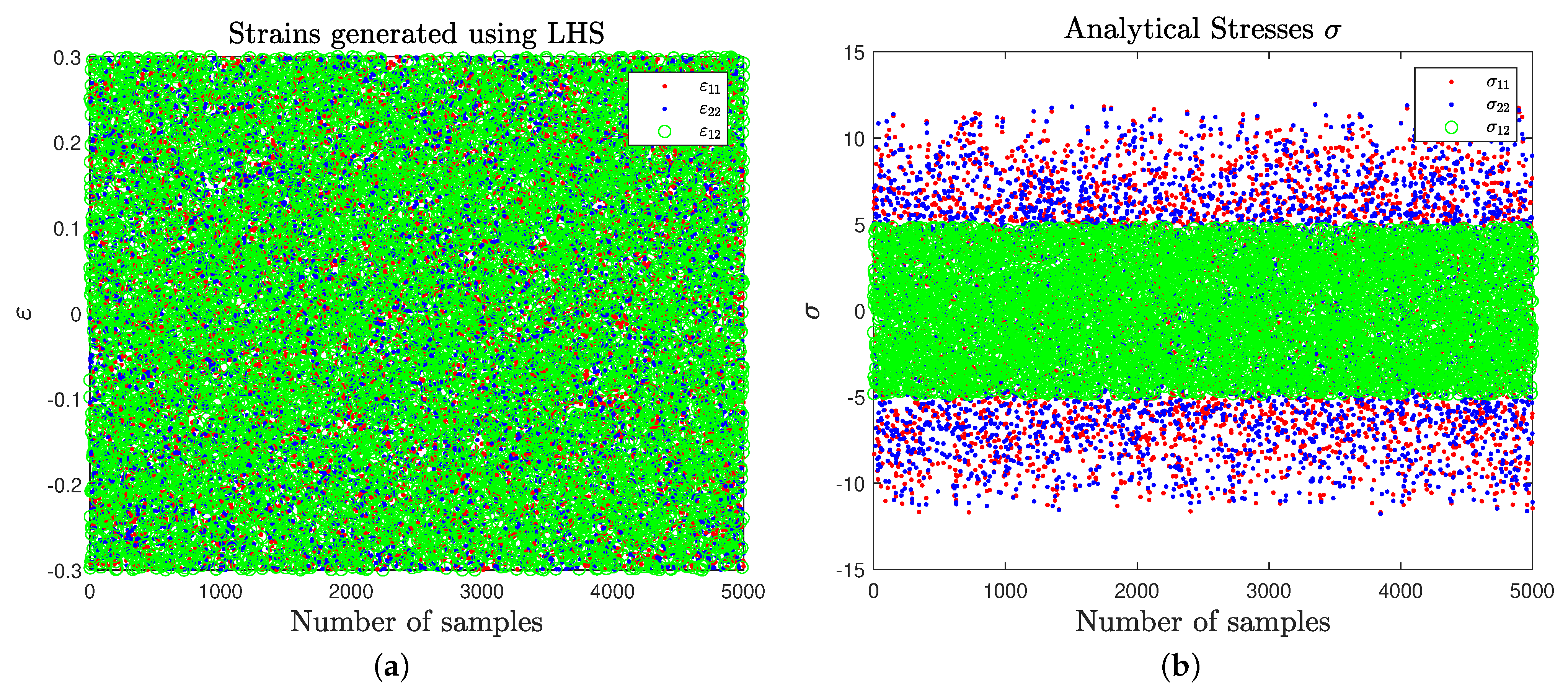
3.1. Data Collection

Determination of the input and output variables for the neural network is the first task for the approximation of elastic behavior by the FFNNs for finite element applications. The strain–stress mapping can be achieved approximated by the FFNNs without considering the loading history since, for the small strain elasticity (elastic deformation), the loading and unloading curve coincide with each other.

3.1.1. Analytical Model

To verify the performance of the NN-based model, a comparison with an analytical model is investigated. The training data are solely collected from the analytical solution instead of using experimental data. To make sure that all the possible values of strains are covered in the training data, the inputs to the analytical model are generated by taking equally spaced points within the given range of strain space. For this purpose, Latin hyper-cube sampling (LHS) is used to generate the data; see Figure 4. As an example of elasticity, the linear elastic model for isotropic material is applied as the target model; a brief overview of this model is summarized below.

3.1.2. Isotropic Elasticity

For isotropic elastic material behavior the Hookean strain energy is assumed to be a quadratic function as follows:

$$\psi \left(\mathit{\epsilon }\right)=\frac{\lambda }{2}{\mathrm{tr}}^2\left[\mathit{\epsilon }\right]+\mu \mathrm{tr}\left[{\mathit{\epsilon }}^2\right],$$

(13)

where $\lambda >0$ and $\mu >0$ are the elastic Lamé constants defined in terms of Young’s modulus E, Poisson’s ratio $\nu$ and the shear modulus G as follows:

$$\lambda =\frac{\nu E}{(1+\nu )(1-2\nu )}\mathrm{and}\mu =G=\frac{E}{2(1+\nu )},$$

(14)

Following the Coleman–Noll procedure, the stress tensor is obtained from the energy function $\psi$ in (13) for isotropic material behavior as follows:

$$\mathit{\sigma }={\partial }_{\mathit{\epsilon }}\psi \left(\mathit{\epsilon }\right)=\lambda \mathrm{tr}\left[\mathit{\epsilon }\right]\mathbf{1}+2\mu \mathit{\epsilon },$$

(15)

hereby, both the stresses $\mathit{\sigma }$ and strains ε are symmetric tensors. For the 2D case, the inputs of the model and their outputs are chosen as the strain and stress components, respectively.

$$\begin{array}{ccc}\hfill \mathrm{Inputs}:& & ({\epsilon }_{xx},{\epsilon }_{yy},{\epsilon }_{xy})\hfill \end{array}$$

(16)

$$\begin{array}{ccc}\hfill \mathrm{Outputs}:& & ({\sigma }_{xx},{\sigma }_{yy},{\sigma }_{xy})\hfill \end{array}$$

(17)

The stresses as output data can be computed using (15) accordingly. The neural network is trained until the stopping criteria is reached. After training, the model is saved. The NN-based elasticity model reads as follows:

$${\mathit{\sigma }}^{\mathit{NN}}=FFNN(\mathit{\epsilon },\mathit{W},\mathit{b}),$$

(18)

where ${\mathit{\sigma }}^{\mathit{NN}}$ is the predicted stress by the FFNN.

As a representative example, we choose the following material parameters for the isotropic-elastic model in the training data collection: Young’s modulus $E=21$ kN/mm${}^2$ and Poisson’s ratio $\nu =0.3$. The data set is split into training (70%), validation (15%), and test (15%) subsets. A feed-forward neural network with an architecture of $3-10-10-3$ is applied. It consists of three neurons for the input and output layer each, and 10 neurons for each of the two hidden layers. The Levenberg–Marquardt algorithm [54] is chosen as the training optimizer. Figure 5 depicts the performance of the neural network model throughout training, where the model performance reaches its optimum at epoch (iteration) 1400 over the scaled data set. This is based on the termination criteria introduced in Section 2. The mean squared error is decreased to $2.2\times {10}^{-16}$, which costs time of 14 m 48 s; see

Table 1. Neural network model specifications—small strain elasticity.

No.	Name	Value	Unit
1.	Number of samples	${10}^4$	−
2.	Training duration	888	s
3.	Training performance	$2.2\times {10}^{-16}$	−

.

3.2. Representative Numerical Examples

In the following, the performance of the proposed machine learning based model is demonstrated through two representative numerical examples. The material parameter used for the isotropic-elastic model in the training data collection and in the finite element analysis using software tools Acegen and AceFEM [55] are as follows: Young’s modulus $E=21$ kN/mm${}^2$ and Poisson’s ratio $\nu =0.3$. Here, also a FFNN with the architecture of $3-10-10-3$ is applied, with 3 neurons for input and output layer each, and 10 neurons for the hidden layers. Furthermore, the Levenberg–Marquardt algorithm is considered the training optimizer. To illustrate the computational methodology, representative tests under different loading conditions are presented.

3.2.1. Compression Test of a Plate

The first model problem is the uniaxial compression test of a rectangular plate. The geometric setup and the loading conditions of the specimen are depicted in Figure 6a. The plate is fixed at the bottom, and a prescribed displacement with an amplitude of $u=-0.04$ mm is imposed at the top surface of the plate with $L=1$ mm. The geometric domain of the structure is discretized by 400 triangular T1 elements, leading to 231 nodes.

The load–deflection curve is depicted in Figure 6b. Next, the stresses computed with the neural network based model is compared with that of Hooke’s model. It can be observed from the contour plot that FFNN predicts the stresses very accurately as shown in Figure 7. This verifies the accuracy of the proposed neural network approach for elasticity problems.

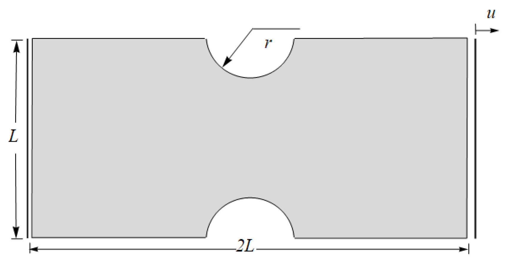
3.2.2. A-Notched Bar in Tension

Next, a tensile test of the A-notched bar as depicted in Figure 8 is conducted. The bar is clamped at the left end and a prescribed displacement with an amplitude of $u=0.02$ mm is imposed on the right end with $L=1$ mm and $r=0.25$ mm. The geometric domain of the structure is discretized by unstructured meshes with a total of 306 triangular T1 elements, leading to 189 nodes.

Similarly, the A-notched bar stresses computed with the neural network model are compared with those of the purely finite element method. It can be seen from the contour plot of both FE and NN formulations that FFNN predicts the stresses very accurately, as shown in Figure 9.

3.2.3. Discussion

From the above-detailed studies, it can be concluded that NN-formulation works well for predicting linear elastic material behavior under different loading conditions and geometries. For a better understanding of the computational efficiency of the neural network model incorporated inside the finite element formulations, a comparison is made with that of finite element analysis based on AceGen generated c code; see

Table 2. AceGen—FEM vs. NN formulations.

No.	Name	FEM	NN	Unit
1.	Evaluation time	3	5	s
2.	Number of formulae	73	92	−
3.	Total size of c code	3414	5982	$\mathrm{bytes}$

.

The evaluation time for the NN embedded model is longer due to the size of the AceGen file (which includes the neural network formulation) and the functions necessary for the computation and normalization of the data required by the NN-model. The positive aspect is that this has to be done once, and after a successful execution, the generated file can be used for finite element simulations. Similarly,

Table 3. 2D plate and A-notched bar—AceFEM simulation report.

		Plate		Bar
No.	Name	FEM	NN	FEM	NN	Unit
1.	Total K and R time	$0.009$	$0.008$	$0.039$	$0.067$	s
2.	CPU Mathematica time	$0.11$	$0.14$	$0.546$	$0.407$	s

provides the simulation report obtained using AceFEM for the 2D plate (Section 3.2.1) and A-notched bar (Section 3.2.2), respectively. Note that the computational effort heavily depends on the machine on which the simulations are running. Therefore, here, only the computation time is compared between the FEM and NN simulations. It can be concluded from the representative examples that although NN accurately predicts the stress–strain relationship, it has no superiority when it comes to the computational effort for the problems in elasticity.

4. Neural Network (NN) Based Elasticity for Fracture Problems

The main objective of this section is to incorporate the NN-based elasticity model (developed in Section 3) within the finite element formulation of phase-field brittle fracture for the sole purpose of efficiently predicting the elasticity part of the phase field. For the sake of brevity, we omit the detailed description of the phase-field modeling of brittle fracture and summarize next the most important equations. For more details, the interested reader is referred to [56,57,58,59,60,61,62,63,64,65,66,67,68,69,70,71,72,73,74,75,76,77,78] and the citations therein.

4.1. Phase-Field Modeling of Brittle Fracture

In this section, we summarize the variational formulations for phase-field modeling of brittle fracture in elastic solids at small strains. The constitutive work density function consists of the following sum:

$$\mathsf{\Psi }(\mathit{\epsilon },d,\nabla d)=g\left(d\right)\psi \left(\mathit{\epsilon }\right)+[1-g\left(d\right)]{\psi }_c+2\frac{{\psi }_c}{\zeta }l\gamma (d,\nabla d),$$

(19)

of a degrading elastic bulk energy $\psi$ depicted in (13) and a contribution due to fracture which represents the accumulated dissipative energy. Hereby, the crack phase-field $d(,t)=0$ represents the unbroken state of the solid and $d(,t)=1$ refers to the fully fractured state. The function $g\left(d\right)={(1-d)}^2$ models the degradation of the stored elastic energy of the solid due to fracture. The crack surface density function is defined as $\gamma (d,\nabla d)=\frac{1}{2l}{d}^2+\frac{l}{2}{|\nabla d|}^2$ in terms of the fracture length scale l that governs the regularization. The formulation (19) depends on two additional fracture parameters, namely, the critical fracture energy ${\psi }_c$ and $\zeta$, which controls the post-critical range after crack initialization, as well documented in [61]. Based on the above-introduced work density function, we derive two governing equations for the coupled problem. The first equation is the stress equilibrium or the quasi-static form of the balance of linear momentum defined as follows:

$$\mathrm{Div}\left[\mathit{\sigma }\right]=\mathbf{0} \mathrm{with} \mathit{\sigma }={\partial }_{\mathit{\epsilon }}\mathsf{\Psi }=g\left(d\right)\tilde{\mathit{\sigma }} \mathrm{and} \tilde{\mathit{\sigma }}=\lambda \mathrm{tr}\left[\mathit{\epsilon }\right]\mathbf{1}+2\mu \mathit{\epsilon }$$

(20)

in terms of the effective stress tensor $\tilde{\mathit{\sigma }}$ and by neglecting volume forces. Following [79], the evolution of the crack phase-field in the domain $\mathsf{\Omega }$ represents the second governing equation as follows:

$$[d-l^2\Delta d]+\eta \dot{d}+(d-1)\mathcal{H}=0 \mathrm{with} \mathcal{H} =\underset{\mathit{s}\in [0,\mathit{t}]}{max}D(\mathit{x},\mathit{s})\ge 0\mathrm{and}D=\zeta {〈\frac{{\psi }^{+}\left({\epsilon }^{+}\right)}{{\psi }_{\mathit{c}}}-1〉}_{+}$$

(21)

along with its homogeneous Neumann boundary condition $\nabla d·\mathit{n}=0$ on $\partial \mathsf{\Omega }$. Here, $\mathit{n}$ is the outward normal on $\partial \mathsf{\Omega }$ and $\eta \ge 0$ is a material parameter that characterizes the artificial/numerical viscosity of the crack propagation. The crack driving force $\mathcal{H}$ is introduced as a local history variable that accounts for the irreversibility of the phase-field evolution by filtering out a maximum value of what is known as the crack driving state function D. This is achieved by introducing the Macaulay bracket ${\langle x\rangle }_{+}=(x+|x\left|\right)/2$. Note that only the tensile/positive part of the elastic energy in (13) is considered for computing the crack driving force. It is defined in terms of the positive strain tensor ${\epsilon }^{+}={\sum }_{a=1}^{\delta }{\langle {\epsilon }_a\rangle }_{+}{\mathit{N}}_a\otimes {\mathit{N}}_a$ with $\delta =2,3$. Here, ${\left\{{\epsilon }_a\right\}}_{a=1..\delta }$ are the principal elastic strains and ${\left\{{\mathit{N}}_a\right\}}_{a=1..\delta }$ are the principal strain directions; for further details on energy decomposition, see [56].

4.2. Neural Network Architecture

In this part, a feed-forward neural network with a similar architecture as that in Section 3 is applied. As a loss function, the mean-squared error (MSE) is considered. Here, also the Levenberg–Marquardt algorithm is chosen as the training optimizer. Since the stress $\mathit{\sigma }$ and strain ε values are on different scales of magnitude, a normalization of the data set is required before training. Thus, the data set is scaled to a comparable range, in which the input and target data are initially scaled to be in the range $[-1,1]$. The training data are collected from the analytical model, similar to the method used in NN-based elasticity; see Section 3. The material parameters used for the creation of the training data set are given in

Table 4. Material parameters used in the numerical examples.

No.	Name	Parameter	Value	Unit
1.	Young’s modulus	E	21	kN/mm${}^2$
2.	Poisson’s ratio	$\nu$	$0.3$	−
3.	Critical fracture energy	${\psi }_c$	$1.35\times {10}^{-3}$	kN/mm${}^2$
4.	Fracture length scale	l	$0.004$	mm
5.	Fracture viscosity	$\eta$	$1\times {10}^{-6}$	N·s/mm${}^2$
6.	Post critical parameter	$\zeta$	$1.0$	−

.

In the following, the performance of the proposed machine learning based model will be examined for the phase-field fracture simulations. Herein, the elasticity is predicted by the neural network. The formulation of the ML-based model substituting the above formulations defines a function in the following format:

$${\tilde{\mathit{\sigma }}}_{NN}(\mathit{\epsilon },d,\mathit{W},\mathit{b})=FFNN(\mathit{\epsilon },\mathit{W},\mathit{b}),$$

(22)

where W is the weight matrix and b is the bias of the neural network.

4.3. Numerical Examples

To illustrate the computational methodology and verify the formulation, two benchmark problems are investigated.

4.3.1. Single-Edge-Notched Tension Test

The first benchmark test considers a square plate ($L=1$ mm) with a horizontal notch placed at the middle height, as plotted in Figure 10 (left). The specimen is discretized using FEM with linear triangles.

A mesh refinement in the expected fracture zone is applied. Furthermore, Figure 10 shows the contour plot of the crack phase-field d for different loading states up to final rupture.

Next, Figure 11 illustrates a comparison between FEM and the Neural Network formulation by calculating the stress–strain relationship using both methods. The predicted stress thoroughly follows the FE solution, which verifies the generalization of the NN model.

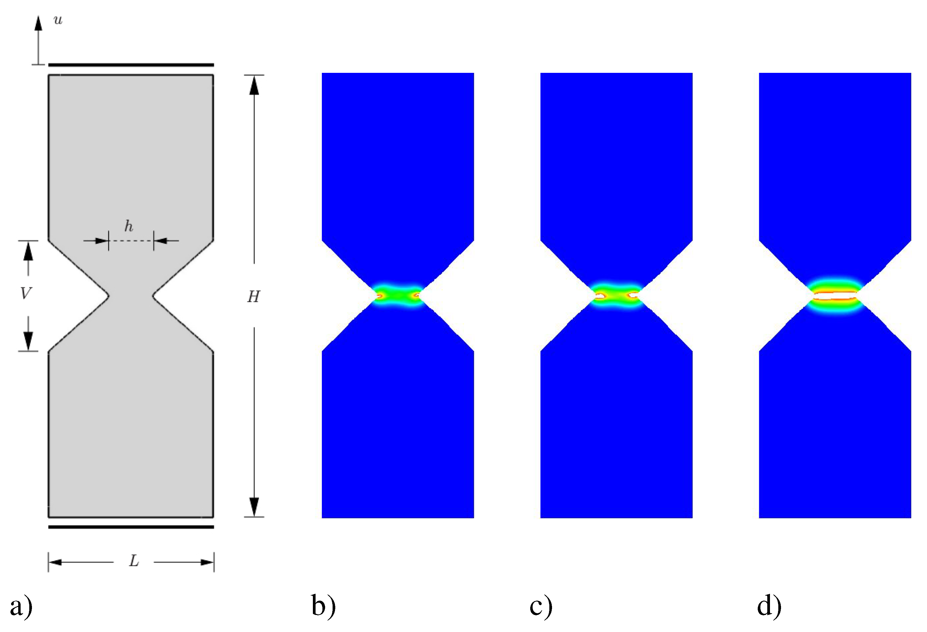
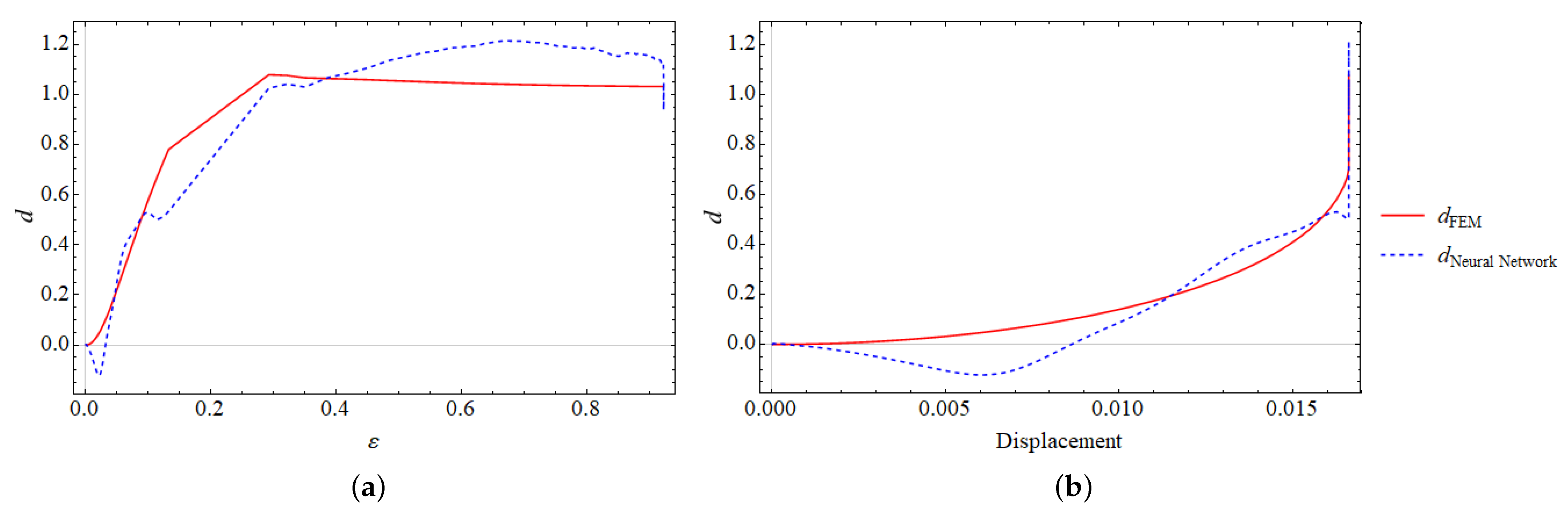
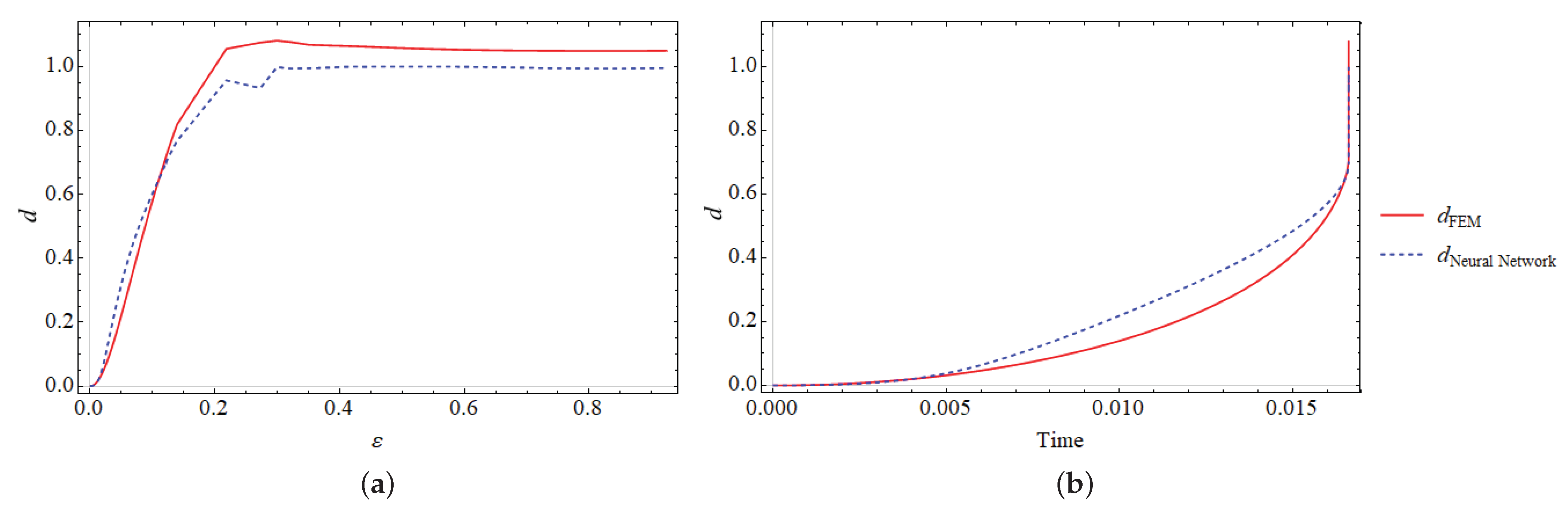
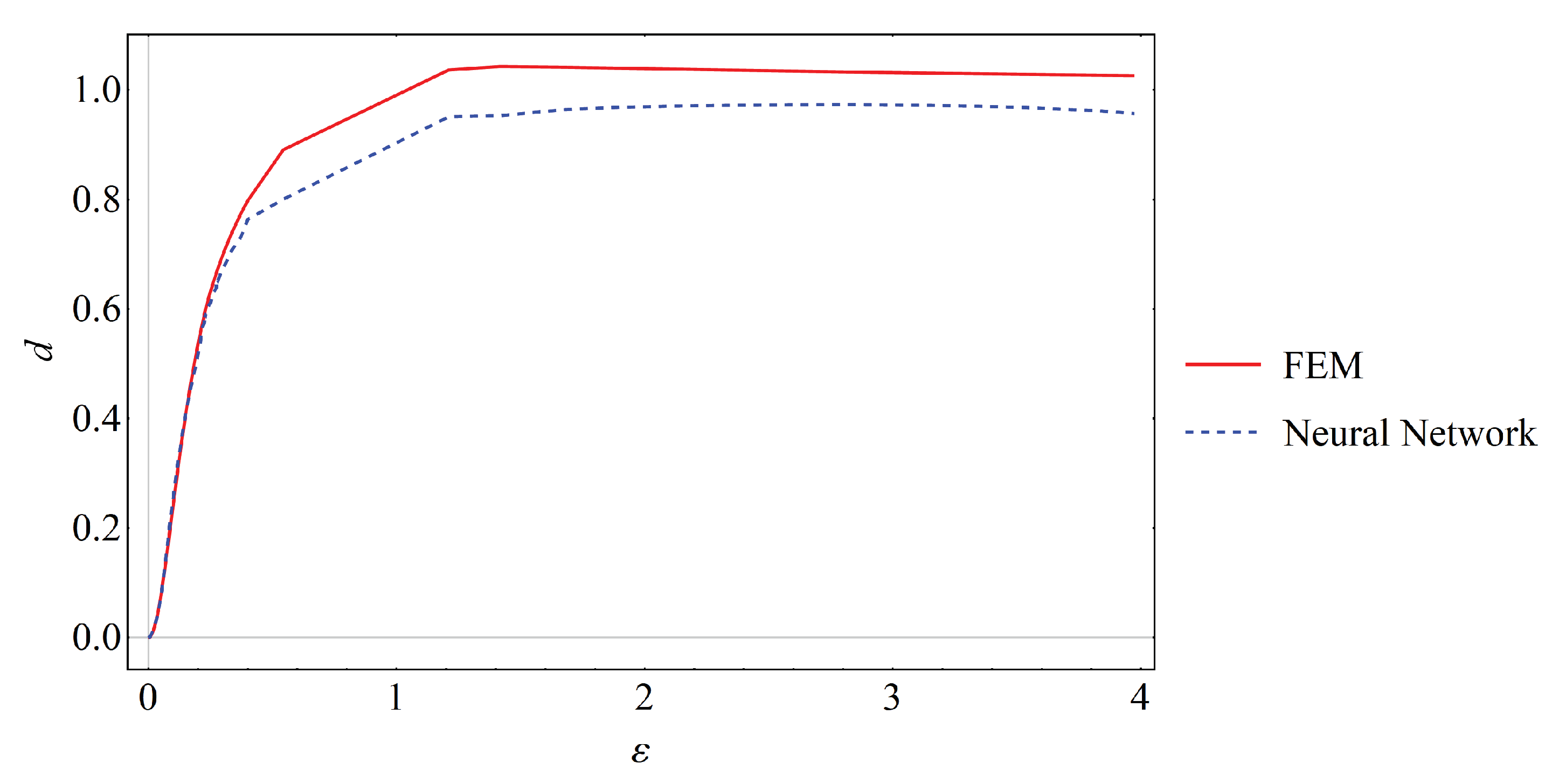
4.3.2. V-Notch Bar in a Tension Test

The second model problem is concerned with analyzing the brittle failure of a V-notch bar under tensile loading. The geometric setup and the loading conditions of the specimen are depicted in Figure 12a. The size of the specimen is chosen to be as follows: $H=1$ mm, $L=0.35$ mm, $h=0.1$ mm and $V=0.24$ mm. The mesh size of the specimen is chosen to be $h_e=0.004$ mm in the expected fracture zone. The computation is performed by applying a displacement with an amplitude of $u=0.02$ mm at the top edge while the bottom edge is fixed in both directions x and y. The material parameters used in this simulation are similar to that of the single edge notched tension test as shown in Table 4. Discretization is achieved by finite element (FEM) formulations with 3-noded linear triangular elements.

The evolution of the crack phase-field d is reported in Figure 12b–d. The crack initiates at the notch tip and successively propagates horizontally from the notches inwards till the final rupture. For visualization of crack surface, deformed regions with a phase-field $d\approx 1$ are plotted in Figure 12.

Next, Figure 13 illustrates a comparison between FEM and NN formulations by calculating the stress–strain relationship using both methods. As in previous examples, predicted stress exactly follows the FE solution.

4.3.3. Discussion

It has been shown that the incorporation of the NN model within FE formulation for the fracture phase-field approach is successful. Herein, the elasticity is approximated using the neural network model rather than the classical methods. Hence, data-driven methods, such as neural networks, are promising in the solution of mechanical problems.

In this regard,

Table 5. AceGen—FEM vs. NN.

No.	Name	FEM	NN	Unit
1.	Evaluation time	8	13	s
2.	Number of formulae	336	358	−
3.	Total size of c code	$\mathrm{15,025}$	$\mathrm{31,629}$	$\mathrm{bytes}$

compares the AceGen generated c code, while

Table 6. SENT and V-notch tests—AceFEM Simulation Report.

		SENT		V-Notch
No.	Name	FEM	NN	FEM	NN	Unit
1.	Total K and R time	11	8	$12.72$	$9.45$	s
2.	CPU Mathematica time	6	$4.5$	5	4	s

provides a brief simulation report of numerical examples to illustrate the computational efficiency of the proposed NN-model. From these tables, it can be observed that, due to the bigger size of the AceGen file, in NN case the evaluation time is longer. On the other hand, the AceFEM simulation report indicates that the total linear solver time, total K and R time, and CPU Mathematica time are smaller when using the NN method; see Table 6. It is worth mentioning that the computational time may vary on different machines; nevertheless, this again verifies the applicability and efficiency of the neural network model.

5. Neural Network (NN)-Based Phase-Field Brittle Fracture

In this last section, a NN-based phase-field model is developed using feed-forward neural networks (FFNNs). The aim here is to embed a neural network-based model inside FEM, which predicts the fracture phase-field d in such a way that this NN-model is able to mimic the behavior of phase-field modeling of brittle fracture to its full potential. Toward this goal, the problem at hand is gradually developed in different steps. These steps demonstrate the scope of applicability and feasibility of this approach. Moreover, it represents a good strategy for confronting possible challenges throughout this study.

5.1. Data Collection

To verify the performance of the NN-based model by comparing their predictions with FE formulations, the training data are exclusively collected from the finite element analysis, i.e., experimental data are not considered. In this regard, both geometries in Figure 10, Figure 11 and Figure 12 are employed for the creation of the data set necessary for training the neural network model. Hereby, data from a specific part of the geometry are considered since the data of interest lie in the region where the crack is expected. For the elasticity part of the phase-field modeling of brittle fracture, the previously trained model is utilized. A second model is also trained solely for predicting the fracture phase-field d. It suffices to state that the accuracy of the predictions (approximations) depends on the complexity of the relationship between the data set for the inputs and outputs. The trained neural network will approximate the mapping between the input and output. Unlike the elasticity model, the relationship between the input and output data in the fracture process is highly nonlinear and complex. To understand these relationships, a sensitivity analysis will provide a better insight into the selection of the proper choice of inputs required to accurately predict the target output.

5.1.1. Sensitivity Analysis

Sensitivity analysis is quite useful in specifying the effect of a particular input on an output under a set of assumptions. Different methods exist in the literature for conducting a thorough sensitivity analysis. However, for our scope of the study, a scatter-plot is sufficient. Such a representation is a qualitative method, which provides no sensitivity index or numerical value. For a full dependency analysis, plots as many as the number of inputs are required.

As an example, Figure 14 illustrates the relationship of total stress due to the degradation of stored elastic energy and total strain. Hereby, the stresses decrease after a certain strain value related to the critical fracture energy ${\psi }_c$ introduced in (19).

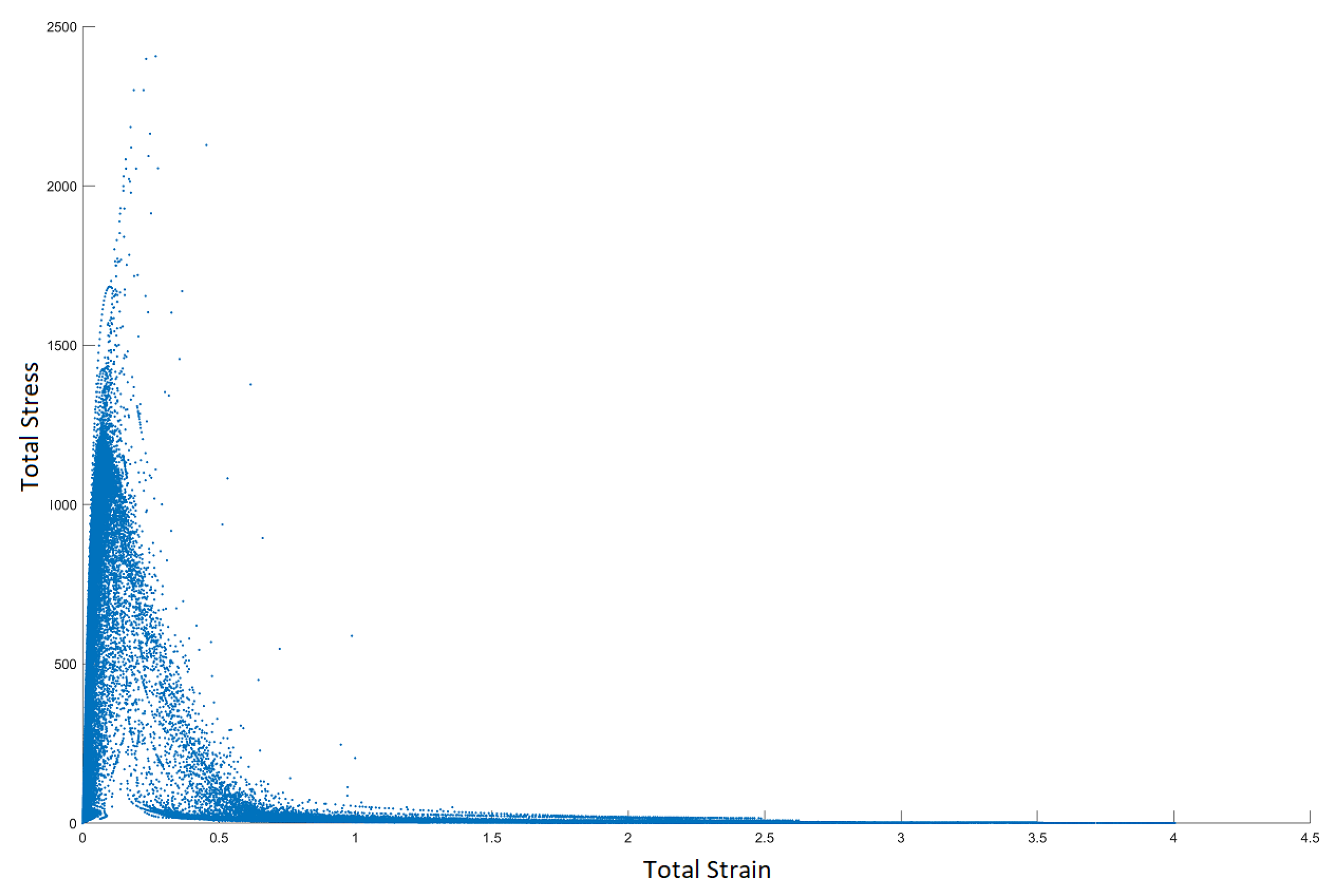
5.1.2. Input and Output Relationship

From the sensitivity analysis, it can be observed that the input and output relationships are highly non-linear. Hence, not much can be learned about the input–output relationship from the scatter-plots of outputs and their respective inputs. Therefore, the model is trained using a different number of input features, and the architecture with better performance was chosen to be embedded in the finite element formulations.

For the prediction of the fracture phase-field d at the current time-step, which would be the output of the NN model, strains, stresses, driving force at the current time-step along with the phase-field d at the previous time step are considered the input to the NN model. Note that the stresses at the current time step have a direct dependency on the current fracture phase-field due to the degradation of stored elastic energy. In this contribution, the stresses are degraded with the previous value of d. This results in a small increase in the global error, i.e., the performance of the neural network model; however, it is still in an acceptable range and yields good results. The formulation of the NN-based phase-field model defines a function in the following format:

$$d_{NN}^t=FFNN({\mathit{\epsilon }}^t,{\mathit{\sigma }}_{NN}^t,d_{NN}^{t-1},{\mathcal{H}}^t,\mathit{W},\mathit{b}),$$

(23)

where $d_{NN}^t$ is the fracture phase-field at the current time-step, ${\mathcal{H}}^t$ is the current driving force, ${\mathit{\epsilon }}^t$ is the current strain with $\mathit{\epsilon }=[{\mathit{\epsilon }}_{xx},{\mathit{\epsilon }}_{yy},{\mathit{\epsilon }}_{xy}]$, and ${\mathit{\sigma }}_{NN}^t$ is the NN-model trained apriori to approximate the stress as follows:

$${\mathit{\sigma }}_{NN}=FFNN(\mathit{\epsilon },\mathit{W},\mathit{b}),$$

(24)

for given strains ε, weight matrix W, and the bias of neural network b.

5.2. Feed-Forward Neural Network

A feed-forward neural network with an architecture of 8-15-15-1 is applied to learn the relationship between input and output datasets. The input layer of the neural network contains 8 neurons (3 strains, 3 stresses, 1 old phase-field and 1 driving force), and the two hidden layers containing 15 neurons each. The output layer contains one neuron which predicts the fracture phase-field d. The Levenberg–Marquardt algorithm [54] is applied as an optimizer for the training of the neural network. The rest of the NN structure follows the same procedures and techniques described in Section 2. After this training, a performance in the order of ${10}^{-5}$ is achieved, as demonstrated in

Table 7. Neural network model specifications.

No.	Name	Value	Unit
1.	Number of samples	165,880	−
2.	Training duration	1200	s
3.	Number of hidden layers	2	−
4.	Number of nodes per hidden layer	15	−
5.	Training performance	$9.65\times {10}^{-5}$	−

.

5.3. Representative Numerical Examples

In the following, the performance of the proposed machine learning based approach is further examined in the prediction of the fracture phase-field d. To this end, the finite element computation is performed by symbolic–numeric programming Mathematica using AceGen and AceFEM packages; see [55]. The trained model weight matrices and biases are incorporated throughout separate functions inside the finite element formulations. Therefore, the calculations can be done without dependency on any other programs (e.g., Matlab machine learning toolbox). After the incorporation of the neural network models within the finite element formulations, AceFEM is used as a finite element environment for the solution of the multi-field problem. The neural network learns from the data, thus the complexity of the NN model is significantly influenced by the data set. To show the contribution of the relevant input (namely previous the NN-based phase-field value $d_{NN}^{t-1}$ at time $t-1$) in the accuracy of the neural network model, two different cases are investigated.

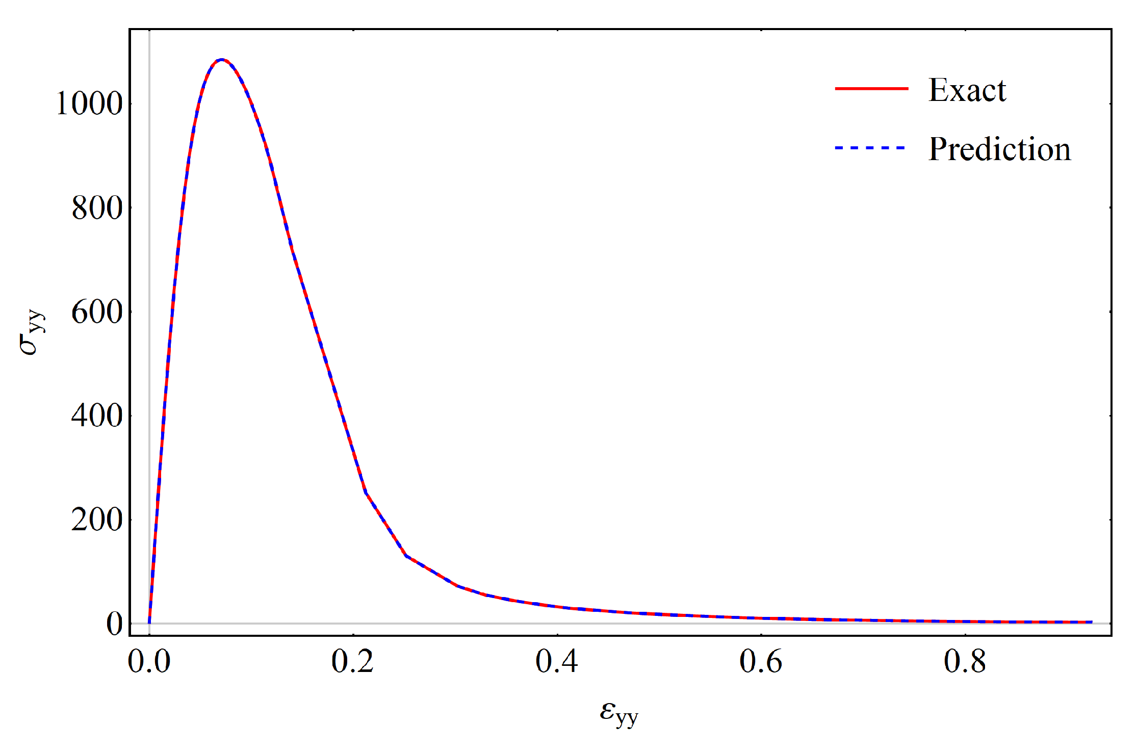
5.3.1. Single-Edge-Notched Test

The same benchmark test depicted in Section 4.3.1 is further examined to verify the computational methodology by comparing the predicted results to that of finite element analysis.

Case 1: The first case considers only stress, strain and, driving force as the input to the neural network model. The formulation of the NN-based phase-field model defines a function in the following format:

$$d_{NN}=FFNN(\mathit{\epsilon },\mathit{\sigma },\mathcal{H},\mathit{W},\mathit{b}),$$

(25)

where stresses are calculated using the finite element method. Only one NN-model is incorporated within the FE-analysis which predicts the phase-field d. The results are promising; however, there are some mismatches between the finite element solution and the NN-model as shown in Figure 15.

Case 2: The second case is similar to the first case; however, there is only one more input to the neural network. Here, the previous value of fracture phase-field d is also considered as an input to the neural network model. The formulation has the following format:

$$d_{NN}^t=FFNN({\mathit{\epsilon }}^t,{\mathit{\sigma }}_{NN}^t,d_{NN}^{t-1},{\mathcal{H}}^t,\mathit{W},\mathit{b}).$$

(26)

In terms of accuracy, this model predicts the relationship between the input and outputs much more accurately than the previous case, see Figure 16. Hence, for the next example, we employ the analysis in Case 2.

In this example, different cases are considered to create the most efficient neural network model for the prediction of the fracture phase-field d and compared in terms of both accuracy and efficiency.

Table 8. AceGen—Case 1 vs. Case 2 (Phase-field).

No.	Name	Case 1	Case 2	Unit
1.	Evaluation time	23	36	s
2.	Number of formulae	444	499	−
3.	Total size of c code	$\mathrm{30,257}$	$\mathrm{55,070}$	$\mathrm{bytes}$

depicts the AceGen generated c code size, while

Table 9. AceFEM—simulation report of Case 1 vs. Case 2 (phase-field).

No.	Name	Case 1	Case 2	Unit
1.	Number of equations	2827	2827	−
2.	Number of steps	198	206	−
3.	Total number of iterations	2246	2475	−
4.	Average iterations/step	$8.2$	$8.5$	−
5.	Total K and R time	$9.6$	$10.4$	s

compares the AceFEM solution times related to the generated code. It can be concluded that incorporating more than one model within the finite element formulation costs more evaluation time during generating the c code. On the other hand, in the AceFEM simulation, there is no significant difference in the total solve time.

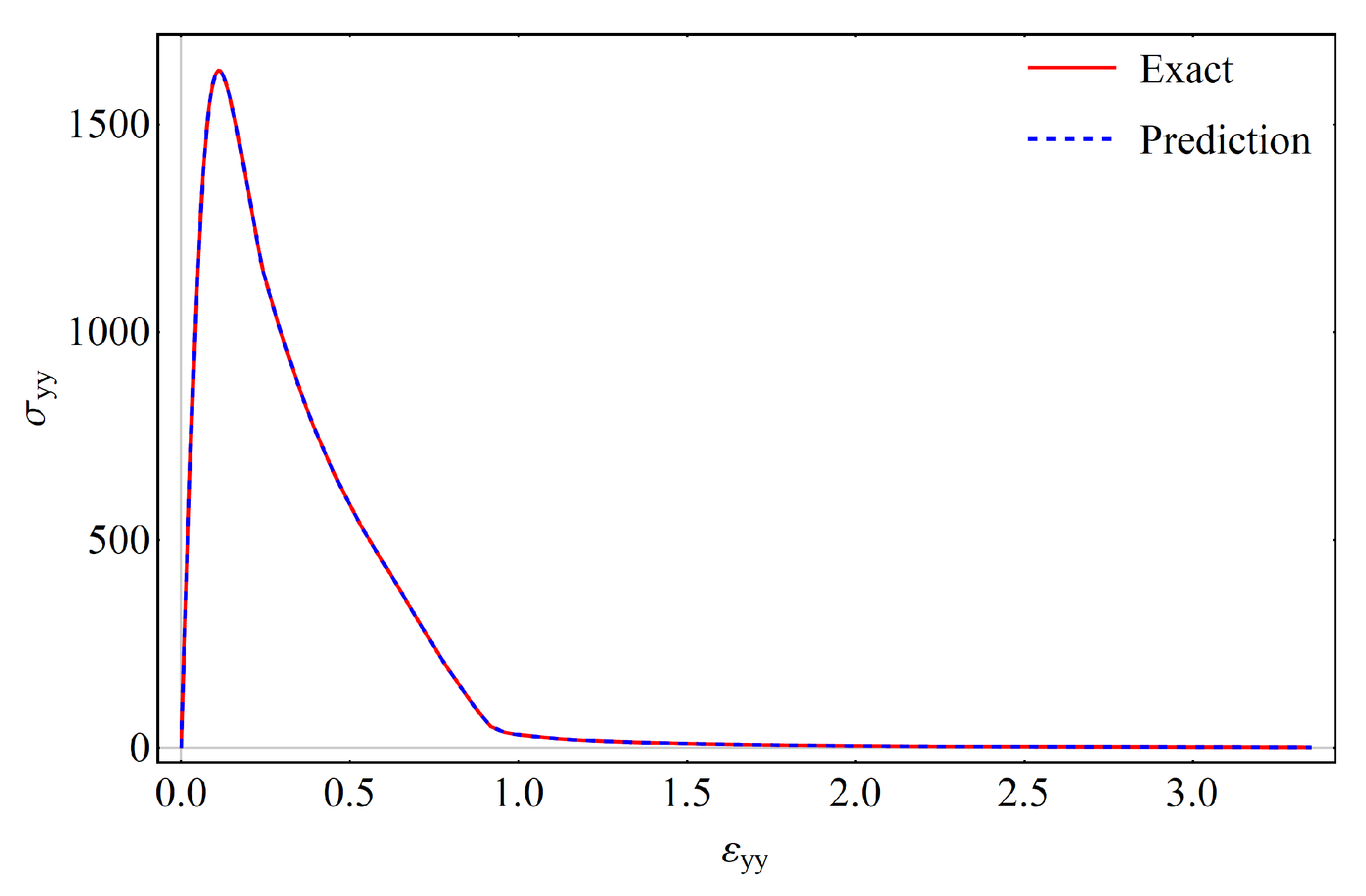
5.3.2. V-Notch Bar in a Tension Test

Further verification of this methodology is illustrated using a V-notched bar in tension. The geometry and boundary conditions of the specimen are similar as before, see Figure 12.

For the analysis, the formulation introduced in Case 2 above is utilized, and the procedure of the previous example is followed. Qualitatively good results are obtained as depicted in Figure 17.

6. Conclusions

This work presented a neural network-based material modeling approach for elasticity and phase field of brittle fracture. The approximation of stresses and fracture phase field in an elastic domain have shown that NN-based approaches can learn the linear and highly non-linear relationship between the input and output data. A commonly used machine learning tool called the “feed-forward neural network” (FFNN) is proven to be efficient for learning the complex input–output relationship, particularly when there is no history dependency between the input and output. Therefore, using NN-based models instead of the conventional numerical procedures to obtain the stresses and fracture phase-field can result in an efficient approach. The automatic symbolic differentiation tool AceGen provides a very convenient way for embedding the neural network formulations within the finite element formulations. The verification of the neural network-based models was conducted by representative numerical examples. We have demonstrated that the NN-based methods, particularly FFNN, can provide accurate and feasible approximations. Accordingly, it can be incorporated in finite element formulations. As our results suggest, the neural network predictions can be identical to the exact solution, provided that the training data set contains all the possible patterns as the target problem. This was achieved for the approximation of stresses in the elastic domain. The question of building a universal NN-based model that requires a universal training data set to be used in a wide range of boundary conditions and different geometries is still open and will be a topic of further research. In this regard, real experimental data of concrete failure underwater (DFG Priority Program SPP 2020 Experimental-Virtual-Lab) will be used as future trained data in the ML approach.

References

1. Wriggers, P. Nonlinear Finite Elements; Springer: Berlin/Heidelberg, Germany; New York, NY, USA, 2008. [Google Scholar]
2. Hughes, T.; Cottrell, J.; Bazilevs, Y. Isogeometric analysis: CAD, finite elements, NURBS, exact geometry and mesh refinement. Comput. Methods Appl. Mech. Eng. 2005, 194, 4135–4195. [Google Scholar] [CrossRef] [Green Version]
3. Beirão Da Veiga, L.; Brezzi, F.; Cangiani, A.; Manzini, G.; Marini, L.D.; Russo, A. Basic principles of virtual element methods. Math. Model. Methods Appl. Sci. 2013, 23, 199–214. [Google Scholar] [CrossRef]
4. Nguyen, L.T.K.; Keip, M.A. A data-driven approach to nonlinear elasticity. Comput. Struct. 2018, 194, 97–115. [Google Scholar] [CrossRef]
5. Leygue, A.; Coret, M.; Réthoré, J.; Stainier, L.; Verron, E. Data-based derivation of material response. Comput. Methods Appl. Mech. Eng. 2018, 331, 184–196. [Google Scholar] [CrossRef]
6. Eggersmann, R.; Kirchdoerfer, T.; Reese, S.; Stainier, L.; Ortiz, M. Model-free data-driven inelasticity. Comput. Methods Appl. Mech. Eng. 2019, 350, 81–99. [Google Scholar] [CrossRef] [Green Version]
7. Carrara, P.; De Lorenzis, L.; Stainier, L.; Ortiz, M. Data-driven fracture mechanics. Comput. Methods Appl. Mech. Eng. 2020, 372, 113390. [Google Scholar] [CrossRef]
8. Bahmani, B.; Sun, W. An accelerated hybrid data-driven/model-based approach for poroelasticity problems with multi-fidelity multi-physics data. arXiv 2020, arXiv:2012.00165. [Google Scholar]
9. Eggersmann, R.; Stainier, L.; Ortiz, M.; Reese, S. Efficient Data Structures for Model-free Data-Driven Computational Mechanics. arXiv 2020, arXiv:2012.00357. [Google Scholar]
10. Bishop, C. Pattern Recognition and Machine Learning; Information Science and Statistics; Springer: New York, NY, USA, 2016. [Google Scholar]
11. Fuhg, J.N.; Böhm, C.; Bouklas, N.; Fau, A.; Wriggers, P.; Marino, M. Model-data-driven constitutive responses: Application to a multiscale computational framework. arXiv 2021, arXiv:2104.02650. [Google Scholar]
12. Aquino, W.; Brigham, J.C. Self-learning finite elements for inverse estimation of thermal constitutive models. Int. J. Heat Mass Transf. 2006, 49, 2466–2478. [Google Scholar] [CrossRef]
13. Lefik, M.; Schrefler, B. Artificial neural network as an incremental non-linear constitutive model for a finite element code. Comput. Methods Appl. Mech. Eng. 2003, 192, 3265–3283. [Google Scholar] [CrossRef]
14. Lefik, M.; Boso, D.; Schrefler, B. Artificial Neural Networks in numerical modelling of composites. Comput. Methods Appl. Mech. Eng. 2009, 198, 1785–1804. [Google Scholar] [CrossRef]
15. Man, H.; Furukawa, T. Neural network constitutive modelling for non-linear characterization of anisotropic materials. Int. J. Numer. Methods Eng. 2011, 85, 939–957. [Google Scholar] [CrossRef]
16. Palau, T.; Kuhn, A.; Nogales, S.; Böhm, H.; Rauh, A. A neural network based elasto-plasticity material model. In ECCOMAS 2012—European Congress on Computational Methods in Applied Sciences and Engineering; e-Book Full Papers; ECCOMAS Proceeding TU: Wien, Austria, 2012; pp. 8861–8870. [Google Scholar]
17. Kessler, B.S.; El-Gizawy, A.S.; Smith, D.E. Incorporating neural network material models within finite element analysis for rheological behavior prediction. J. Press. Vessel Technol. 2007, 129, 58–65. [Google Scholar] [CrossRef]
18. Zhang, X.; Garikipati, K. Machine learning materials physics: Multi-resolution neural networks learn the free energy and nonlinear elastic response of evolving microstructures. Comput. Methods Appl. Mech. Eng. 2020, 372, 113362. [Google Scholar] [CrossRef]
19. Lu, L.; Meng, X.; Mao, Z.; Karniadakis, G.E. DeepXDE: A deep learning library for solving differential equations. SIAM Rev. 2021, 63, 208–228. [Google Scholar] [CrossRef]
20. Ghaboussi, J.; Garrett, J., Jr.; Wu, X. Knowledge-based modeling of material behavior with neural networks. J. Eng. Mech. 1991, 117, 132–153. [Google Scholar] [CrossRef]
21. Shin, H.; Pande, G. On self-learning finite element codes based on monitored response of structures. Comput. Geotech. 2000, 27, 161–178. [Google Scholar] [CrossRef]
22. Aquino, W.; Brigham, J.C. Neural networks in mechanics of structures and materials—New results and prospects of applications. Comput. Struct. 2001, 79, 2261–2276. [Google Scholar]
23. Waszczyszyn, Z. Neural Networks in Plasticity—Some New Results and Prospects of Applications. In Proceedings of the ECCOMAS—European Congress on Computational Methods in Applied Sciences and Engineering, Barcelona, Spain, 11–14 September 2000. [Google Scholar]
24. Yagawa, G.; Okuda, H. Neural networks in computational mechanics. Arch. Comput. Methods Eng. 1996, 3, 435–512. [Google Scholar] [CrossRef]
25. Theocaris, P.S.; Panagiotopoulos, P. Generalised hardening plasticity approximated via anisotropic elasticity: A neural network approach. Comput. Methods Appl. Mech. Eng. 1995, 125, 123–139. [Google Scholar] [CrossRef]
26. Theocaris, P.; Panagiotopoulos, P. Neural networks for computing in fracture mechanics. Methods and prospects of applications. Comput. Methods Appl. Mech. Eng. 1993, 106, 213–228. [Google Scholar] [CrossRef]
27. Göküzüm, F.S.; Nguyen, L.T.K.; Keip, M.A. An Artificial Neural Network Based Solution Scheme for Periodic Computational Homogenization of Electrostatic Problems. Math. Comput. Appl. 2019, 24, 40. [Google Scholar] [CrossRef] [Green Version]
28. Khatir, S.; Wahab, M.A. Fast simulations for solving fracture mechanics inverse problems using POD-RBF XIGA and Jaya algorithm. Eng. Fract. Mech. 2019, 205, 285–300. [Google Scholar] [CrossRef]
29. Nguyen-Thanh, V.M.; Zhuang, X.; Rabczuk, T. A deep energy method for finite deformation hyperelasticity. Eur. J. Mech. A/Solids 2020, 80, 103874. [Google Scholar] [CrossRef]
30. Wessels, H.; Weißenfels, C.; Wriggers, P. The neural particle method—An updated Lagrangian physics informed neural network for computational fluid dynamics. Comput. Methods Appl. Mech. Eng. 2020, 368, 113127. [Google Scholar] [CrossRef]
31. Settgast, C.; Hütter, G.; Kuna, M.; Abendroth, M. A hybrid approach to simulate the homogenized irreversible elastic–plastic deformations and damage of foams by neural networks. Int. J. Plast. 2020, 126, 102624. [Google Scholar] [CrossRef] [Green Version]
32. Minh Nguyen-Thanh, V.; Trong Khiem Nguyen, L.; Rabczuk, T.; Zhuang, X. A surrogate model for computational homogenization of elastostatics at finite strain using high-dimensional model representation-based neural network. Int. J. Numer. Methods Eng. 2020, 121, 4811–4842. [Google Scholar] [CrossRef]
33. Götz, M.; Leichsenring, F.; Kropp, T.; Müller, P.; Falk, T.; Graf, W.; Kaliske, M.; Drossel, W.G. Data Mining and Machine Learning Methods Applied to 3 A Numerical Clinching Model. Comput. Model. Eng. Sci. 2018, 117, 387–423. [Google Scholar] [CrossRef] [Green Version]
34. Koeppe, A.; Bamer, F.; Markert, B. An intelligent nonlinear meta element for elastoplastic continua: Deep learning using a new Time-distributed Residual U-Net architecture. Comput. Methods Appl. Mech. Eng. 2020, 366, 113088. [Google Scholar] [CrossRef]
35. Fernández, M.; Rezaei, S.; Mianroodi, J.R.; Fritzen, F.; Reese, S. Application of artificial neural networks for the prediction of interface mechanics: A study on grain boundary constitutive behavior. Adv. Model. Simul. Eng. Sci. 2020, 7, 1–27. [Google Scholar] [CrossRef]
36. Hamdia, K.M.; Zhuang, X.; Rabczuk, T. An efficient optimization approach for designing machine learning models based on genetic algorithm. Neural Comput. Appl. 2021, 33, 1923–1933. [Google Scholar] [CrossRef]
37. Heider, Y.; Wang, K.; Sun, W. SO(3)-invariance of informed-graph-based deep neural network for anisotropic elastoplastic materials. Comput. Methods Appl. Mech. Eng. 2020, 363, 112875. [Google Scholar] [CrossRef]
38. Khatir, S.; Boutchicha, D.; Le Thanh, C.; Tran-Ngoc, H.; Nguyen, T.; Abdel-Wahab, M. Improved ANN technique combined with Jaya algorithm for crack identification in plates using XIGA and experimental analysis. Theor. Appl. Fract. Mech. 2020, 107, 102554. [Google Scholar] [CrossRef]
39. Samaniego, E.; Anitescu, C.; Goswami, S.; Nguyen-Thanh, V.M.; Guo, H.; Hamdia, K.; Zhuang, X.; Rabczuk, T. An energy approach to the solution of partial differential equations in computational mechanics via machine learning: Concepts, implementation and applications. Comput. Methods Appl. Mech. Eng. 2020, 362, 112790. [Google Scholar] [CrossRef] [Green Version]
40. Fuchs, A.; Heider, Y.; Wang, K.; Sun, W.; Kaliske, M. DNN2: A hyper-parameter reinforcement learning game for self-design of neural network based elasto-plastic constitutive descriptions. Comput. Struct. 2021, 249, 106505. [Google Scholar] [CrossRef]
41. Heider, Y.; Suh, H.S.; Sun, W. An offline multi-scale unsaturated poromechanics model enabled by self-designed/self-improved neural networks. Int. J. Numer. Anal. Methods Geomech. 2021, 45, 1212–1237. [Google Scholar] [CrossRef]
42. Zhang, X.; Garikipati, K. Bayesian neural networks for weak solution of PDEs with uncertainty quantification. arXiv 2021, arXiv:cs.CE/2101.04879. [Google Scholar]
43. Seguini, M.; Khatir, S.; Boutchicha, D.; Nedjar, D.; Wahab, M.A. Crack prediction in pipeline using ANN-PSO based on numerical and experimental modal analysis. Smart Struct. Syst. 2021, 27, 507. [Google Scholar]
44. Ghaboussi, J.; Pecknold, D.A.; Zhang, M.; Haj-Ali, R.M. Autoprogressive training of neural network constitutive models. Int. J. Numer. Methods Eng. 1998, 42, 105–126. [Google Scholar] [CrossRef]
45. Ghaboussi, J.; Wu, X.; Kaklauskas, G. Neural Network Material Modelling. Statyba 1999, 5, 250–257. [Google Scholar] [CrossRef] [Green Version]
46. Hashash, Y.M.; Jung, S.; Ghaboussi, J. Numerical implementation of a neural network based material model in finite element analysis. Int. J. Numer. Methods Eng. 2004, 59, 989–1005. [Google Scholar] [CrossRef]
47. Huang, D.; Fuhg, J.N.; Weißenfels, C.; Wriggers, P. A machine learning based plasticity model using proper orthogonal decomposition. Comput. Methods Appl. Mech. Eng. 2020, 365, 113008. [Google Scholar] [CrossRef] [Green Version]
48. Abueidda, D.W.; Almasri, M.; Ammourah, R.; Ravaioli, U.; Jasiuk, I.M.; Sobh, N.A. Prediction and optimization of mechanical properties of composites using convolutional neural networks. Compos. Struct. 2019, 227, 111264. [Google Scholar] [CrossRef] [Green Version]
49. Vlassis, N.; Ma, R.; Sun, W. Geometric deep learning for computational mechanics Part I: Anisotropic Hyperelasticity. Comput. Methods Appl. Mech. Eng. 2020, 371, 113299. [Google Scholar] [CrossRef]
50. Yang, Z.; Yabansu, Y.C.; Al-Bahrani, R.; Liao, W.K.; Choudhary, A.N.; Kalidindi, S.R.; Agrawal, A. Deep learning approaches for mining structure-property linkages in high contrast composites from simulation datasets. Comput. Mater. Sci. 2018, 151, 278–287. [Google Scholar] [CrossRef]
51. Frankel, A.L.; Jones, R.E.; Alleman, C.; Templeton, J.A. Predicting the mechanical response of oligocrystals with deep learning. Comput. Mater. Sci. 2019, 169, 109099. [Google Scholar] [CrossRef] [Green Version]
52. Rao, C.; Liu, Y. Three-dimensional convolutional neural network (3D-CNN) for heterogeneous material homogenization. Comput. Mater. Sci. 2020, 184, 109850. [Google Scholar] [CrossRef]
53. Goodfellow, I.; Bengio, Y.; Courville, A.; Bengio, Y. Deep Learning; MIT Press: Cambridge, MA, USA, 2016; Volume 1. [Google Scholar]
54. Hagan, M.; Menhaj, M. Training Feedforward Networks with the Marquardt Algorithm. IEEE Trans. Neural Netw. 1994, 5, 989–993. [Google Scholar] [CrossRef]
55. Korelc, J.; Wriggers, P. Automation of Finite Element Methods; Springer: Berlin/Heidelberg, Germany, 2016. [Google Scholar] [CrossRef]
56. Miehe, C.; Welschinger, F.; Hofacker, M. Thermodynamically consistent phase-field models of fracture: Variational principles and multi-field FE implementations. Int. J. Numer. Methods Eng. 2010, 83, 1273–1311. [Google Scholar] [CrossRef]
57. Aldakheel, F.; Mauthe, S.; Miehe, C. Towards Phase Field Modeling of Ductile Fracture in Gradient-Extended Elastic-Plastic Solids. Proc. Appl. Math. Mech. 2014, 14, 411–412. [Google Scholar] [CrossRef]
58. Ambati, M.; Gerasimov, T.; De Lorenzis, L. A review on phase-field models of brittle fracture and a new fast hybrid formulation. Comput. Mech. 2015, 55, 383–405. [Google Scholar] [CrossRef]
59. Kuhn, C.; Müller, R. A continuum phase field model for fracture. Eng. Fract. Mech. 2010, 77, 3625–3634. [Google Scholar] [CrossRef]
60. Hesch, C.; Weinberg, K. Thermodynamically consistent algorithms for a finite-deformation phase-field approach to fracture. Int. J. Numer. Methods Eng. 2014, 99, 906–924. [Google Scholar] [CrossRef]
61. Aldakheel, F. Mechanics of Nonlocal Dissipative Solids: Gradient Plasticity and Phase Field Modeling of Ductile Fracture. Ph.D. Thesis, University of Stuttgart, Stuttgart, Germany, 2016. [Google Scholar] [CrossRef]
62. Gültekin, O.; Dal, H.; Holzapfel, G.A. A phase-field approach to model fracture of arterial walls: Theory and finite element analysis. Comput. Methods Appl. Mech. Eng. 2016, 312, 542–566. [Google Scholar] [CrossRef]
63. Paggi, M.; Reinoso, J. Revisiting the problem of a crack impinging on an interface: A modeling framework for the interaction between the phase field approach for brittle fracture and the interface cohesive zone model. Comput. Methods Appl. Mech. Eng. 2017, 321, 145–172. [Google Scholar] [CrossRef] [Green Version]
64. Borden, M.J.; Hughes, T.J.R.; Landis, C.M.; Verhoosel, C.V. A higher-order phase-field model for brittle fracture: Formulation and analysis within the isogeometric analysis framework. Comput. Methods Appl. Mech. Eng. 2014, 273, 100–118. [Google Scholar] [CrossRef]
65. Teichtmeister, S.; Kienle, D.; Aldakheel, F.; Keip, M.A. Phase field modeling of fracture in anisotropic brittle solids. Int. J. Non-Linear Mech. 2017, 97, 1–21. [Google Scholar] [CrossRef]
66. Ehlers, W.; Luo, C. A phase-field approach embedded in the Theory of Porous Media for the description of dynamic hydraulic fracturing. Comput. Methods Appl. Mech. Eng. 2017, 315, 348–368. [Google Scholar] [CrossRef]
67. Zhang, X.; Vignes, C.; Sloan, S.W.; Sheng, D. Numerical evaluation of the phase-field model for brittle fracture with emphasis on the length scale. Comput. Mech. 2017, 59, 737–752. [Google Scholar] [CrossRef]
68. Wick, T. Multiphysics Phase-Field Fracture: Modeling, Adaptive Discretizations, and Solvers; Walter de Gruyter GmbH & Co. KG: Berlin, Germany; Boston, MA, USA, 2020; Volume 28. [Google Scholar]
69. Pise, M.; Bluhm, J.; Schröder, J. Elasto-plastic phase-field model of hydraulic fracture in saturated binary porous media. Int. J. Multiscale Comput. Eng. 2019, 17, 201–221. [Google Scholar] [CrossRef]
70. Seleš, K.; Lesičar, T.; Tonković, Z.; Sorić, J. A residual control staggered solution scheme for the phase-field modeling of brittle fracture. Eng. Fract. Mech. 2019, 205, 370–386. [Google Scholar] [CrossRef]
71. Kienle, D.; Aldakheel, F.; Keip, M.A. A finite-strain phase-field approach to ductile failure of frictional materials. Int. J. Solids Struct. 2019, 172, 147–162. [Google Scholar] [CrossRef]
72. Makvandi, R.; Duczek, S.; Juhre, D. A phase-field fracture model based on strain gradient elasticity. Eng. Fract. Mech. 2019, 220, 106648. [Google Scholar] [CrossRef]
73. Yin, B.; Steinke, C.; Kaliske, M. Formulation and implementation of strain rate-dependent fracture toughness in context of the phase-field method. Int. J. Numer. Methods Eng. 2020, 121, 233–255. [Google Scholar] [CrossRef]
74. Mesgarnejad, A.; Imanian, A.; Karma, A. Phase-field models for fatigue crack growth. Theor. Appl. Fract. Mech. 2019, 103, 102282. [Google Scholar] [CrossRef] [Green Version]
75. Dittmann, M.; Aldakheel, F.; Schulte, J.; Schmidt, F.; Krüger, M.; Wriggers, P.; Hesch, C. Phase-field modeling of porous-ductile fracture in non-linear thermo-elasto-plastic solids. Comput. Methods Appl. Mech. Eng. 2020, 361, 112730. [Google Scholar] [CrossRef]
76. Denli, F.A.; Gültekin, O.; Holzapfel, G.A.; Dal, H. A phase-field model for fracture of unidirectional fiber-reinforced polymer matrix composites. Comput. Mech. 2020, 65, 1149–1166. [Google Scholar] [CrossRef]
77. Heider, Y.; Sun, W. A phase field framework for capillary-induced fracture in unsaturated porous media: Drying-induced vs. hydraulic cracking. Comput. Methods Appl. Mech. Eng. 2020, 359, 112647. [Google Scholar] [CrossRef] [Green Version]
78. Seiler, M.; Keller, S.; Kashaev, N.; Klusemann, B.; Kästner, M. Phase-field modelling for fatigue crack growth under laser-shock-peening-induced residual stresses. Arch. Appl. Mech. 2020. [Google Scholar] [CrossRef]
79. Miehe, C.; Hofacker, M.; Schänzel, L.M.; Aldakheel, F. Phase Field Modeling of Fracture in Multi-Physics Problems. Part II. Brittle-to-Ductile Failure Mode Transition and Crack Propagation in Thermo-Elastic-Plastic Solids. Comput. Methods Appl. Mech. Eng. 2015, 294, 486–522. [Google Scholar] [CrossRef]
Figure 1. Schematic representation of an artificial neuron.
Applsci 11 06483 g001
Figure 2. Transfer functions. Left: Sigmoid transfer function; middle: Hyperbolic-tangent transfer function; and right: Purelin transfer function.
Applsci 11 06483 g002
Figure 3. A fully-connected feed-forward neural network. The input layer x has three features, each of the two hidden layers has 10 neurons and the output layer y ^ has three outputs.
Applsci 11 06483 g003
Figure 4. Analytically generated data set. (a) Input data—2D strains ε and (b) output data—2D stresses σ [kN/mm 2 ].
Applsci 11 06483 g004
Figure 5. Mean squared error (MSE) of neural network model with two hidden layers.
Applsci 11 06483 g005
Figure 6. Compression test of a plate. (a) Geometry, boundary conditions, and FEM discretization. (b) Load–deflection curve using finite element formulation.
Applsci 11 06483 g006
Figure 7. Compression test of a plate. Contour plot of the stresses σ y y [N/mm 2 ] with (a) finite element method, and (b) neural network formulation.
Applsci 11 06483 g007
Figure 8. A-notched bar in tension. Geometry and boundary conditions.
Applsci 11 06483 g008
Figure 9. A-notched bar in tension. Contour plot of the stresses σ x x [N/mm 2 ] with (a) finite element method and (b) neural network formulation.
Applsci 11 06483 g009
Figure 10. Single-edge notched test (SENT). Geometry and contour plots of the fracture phase-field d for different loading states up to final failure using FEM with 3-noded linear triangular elements.
Applsci 11 06483 g010
Figure 11. Single-edge notched test (SENT). Validation of stress–strain behavior with NN formulation against FE formulation. The stress unit is [N/mm 2 ].
Applsci 11 06483 g011
Figure 12. V-notch bar in tension. (a) Geometry and boundary conditions. (bd) FEM: Contour plots of the fracture phase-field d evolution for different loading states up to final failure.
Applsci 11 06483 g012
Figure 13. V-notch bar in tension. Validation of stress–strain behavior with NN formulation against FEM. The stress unit is [N/mm 2 ].
Applsci 11 06483 g013
Figure 14. Scatter plots. Total stress vs. total strain throughout the finite element simulation of the phase-field modeling of brittle fracture. The stress unit is [N/mm 2 ].
Applsci 11 06483 g014
Figure 15. Case 1: Single-edge notched tension test. Fracture phase-field d curves versus strain ε in (a) and vs. displacement u in (b).
Applsci 11 06483 g015
Figure 16. Case 2: Single-edge notched tension test. Fracture phase-field d curves versus strain ε in (a) and vs. time t in (b).
Applsci 11 06483 g016
Figure 17. Case 2: V-notched tension test. Fracture phase-field d curves versus the strain ε.
Applsci 11 06483 g017