Analysis of Flow Characteristics and Effects of Turbulence Models for the Butterfly Valve


Abstract
1. Introduction
2. Theory
2.1. Turbulence Model
2.1.1. Two-Equation Model of Launder and Sharma l
2.1.2. Two-Equation Model of Wilcox
2.1.3. Shear Stress Transport (SST) Model
2.2. Flow Coefficient of a Valve
3. Numerical Implementation
3.1. Calculation Conditions
3.2. Mesh Dependence Study
4. Results and Discussion
4.1. Flow Coefficient
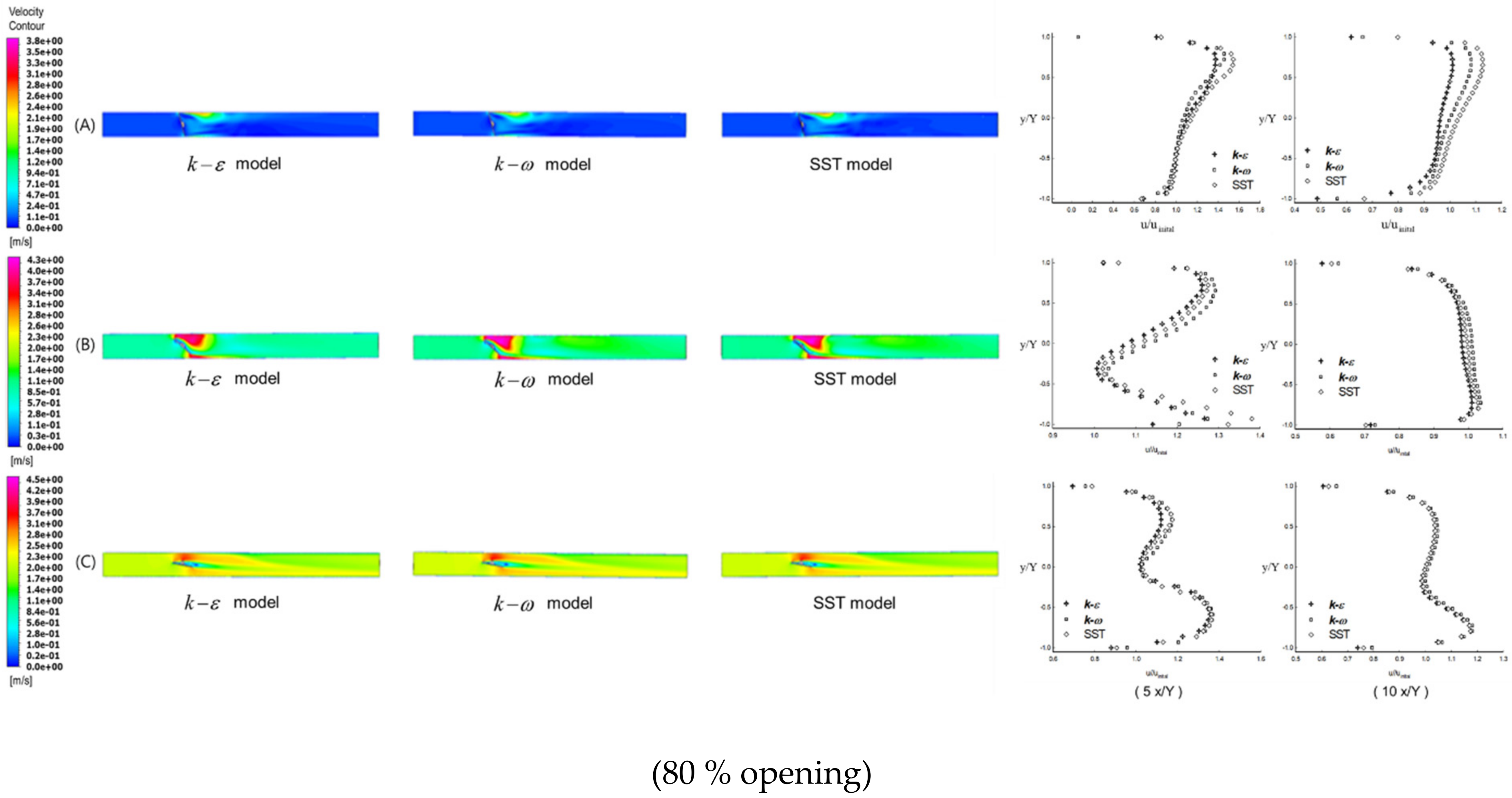
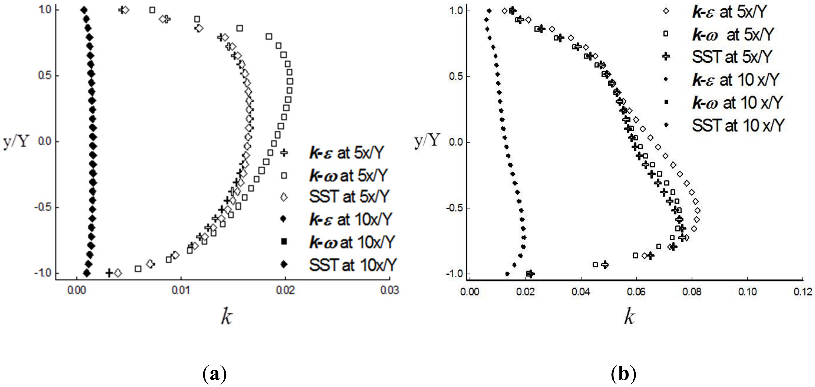
4.2. Flow Behavior
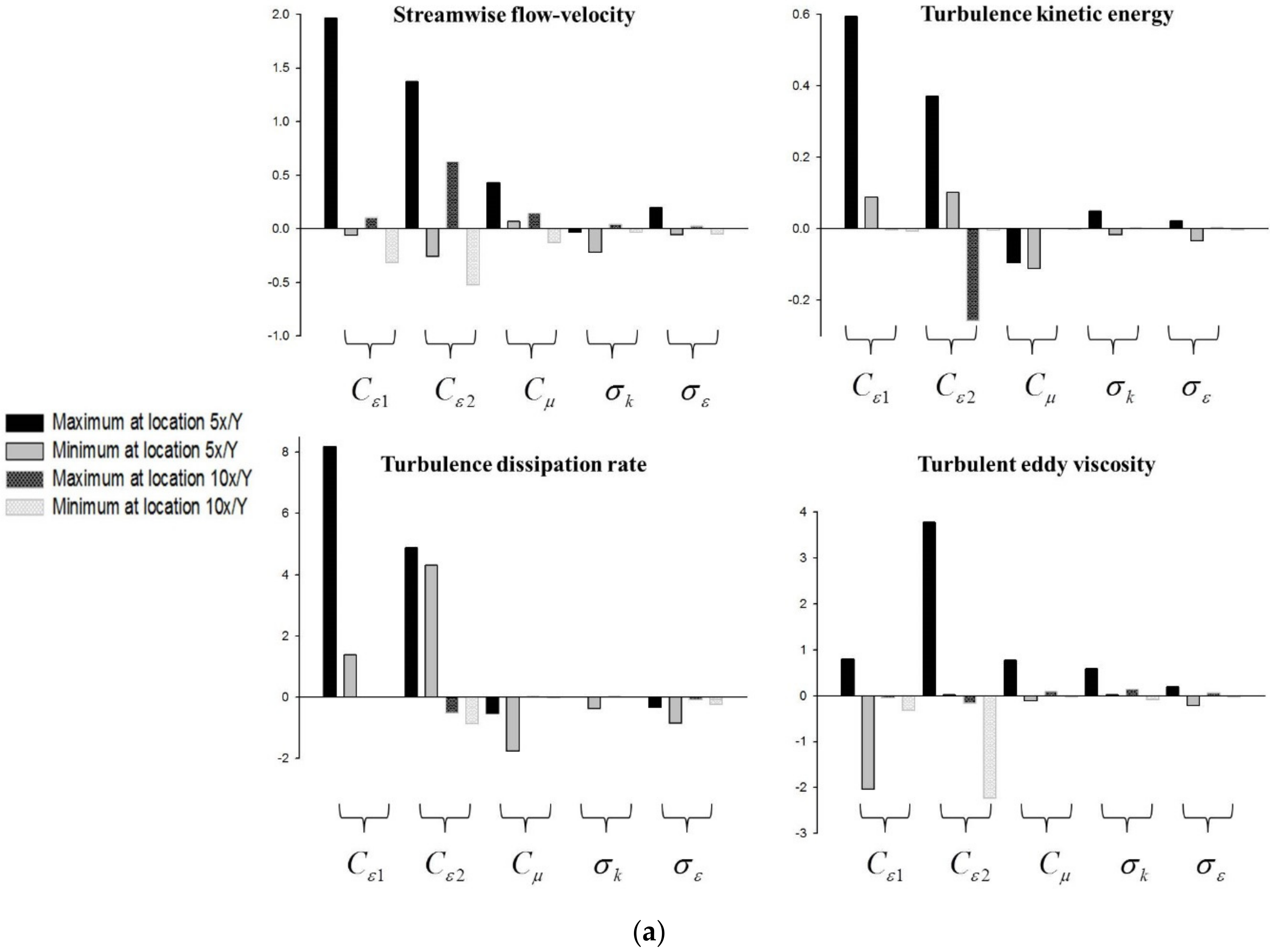
5. Sensitivity Analysis
5.1. Sensitivity Result of Two-Equation Model
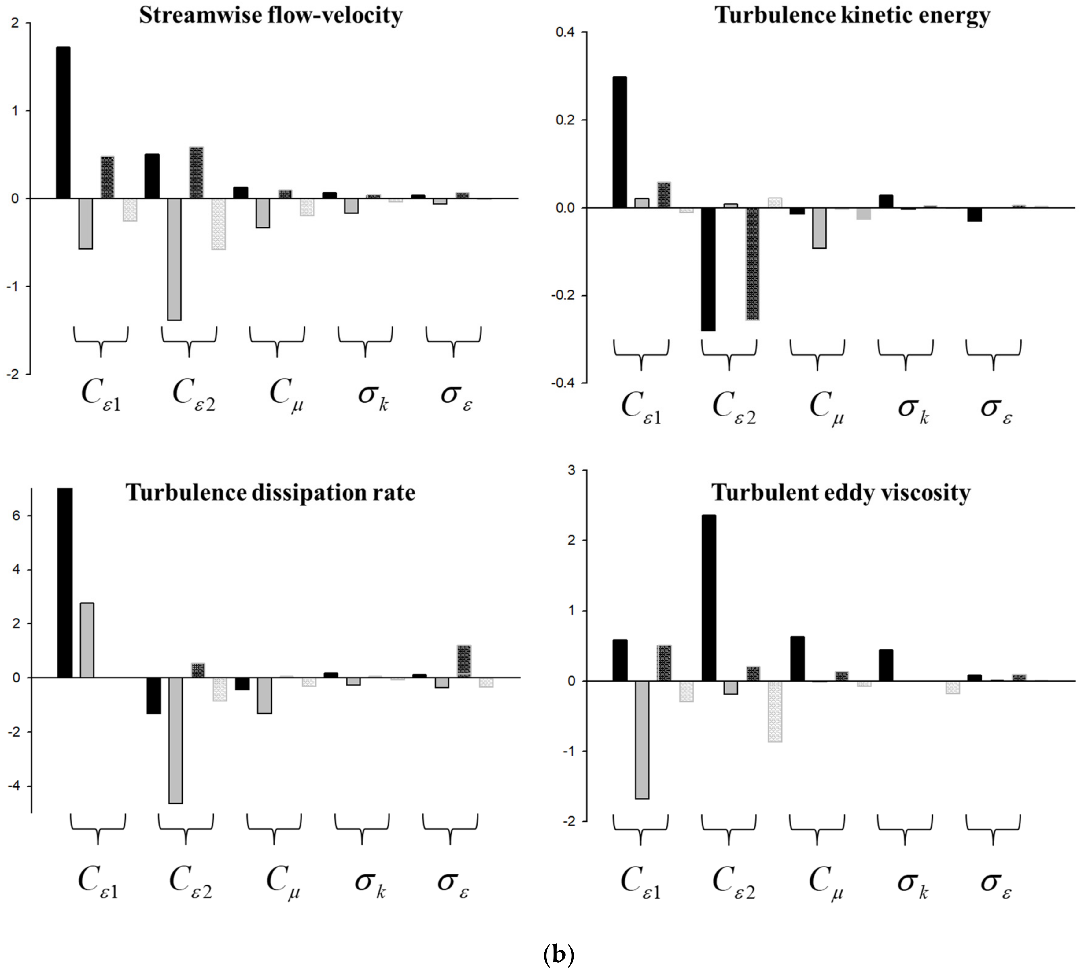
5.2. Sensitivity Result of Two-Equation Model
6. Concluding Remarks
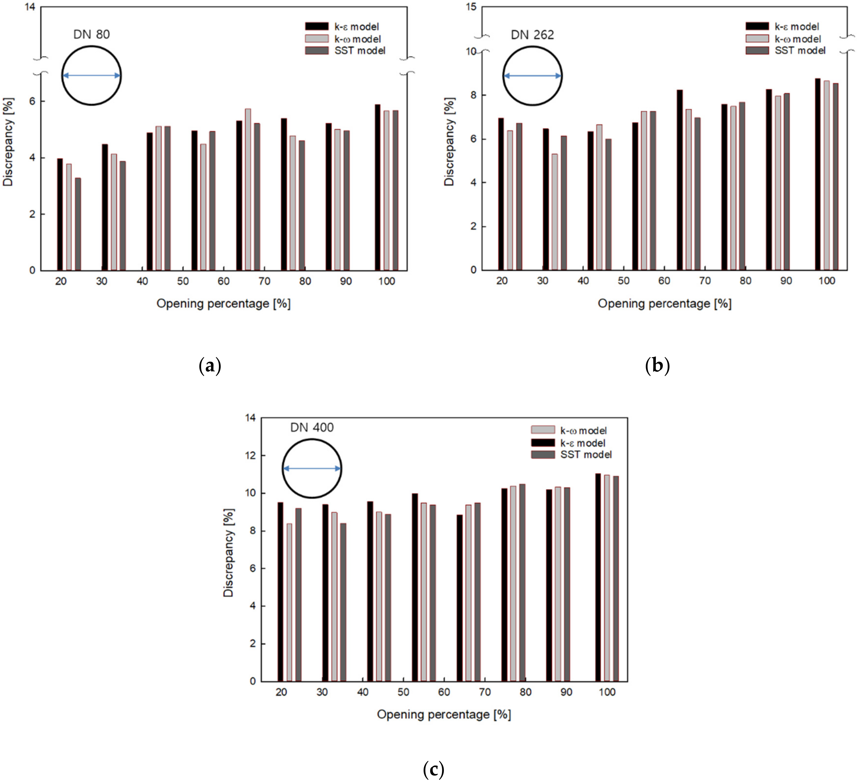
- With different-sized valves, discrepancies between numerical and experimental results for the flow coefficient were observed with different disc openings. The discrepancies increased with increasing valve size, and different degrees of discrepancy were observed with disc opening percentage for each valve size.
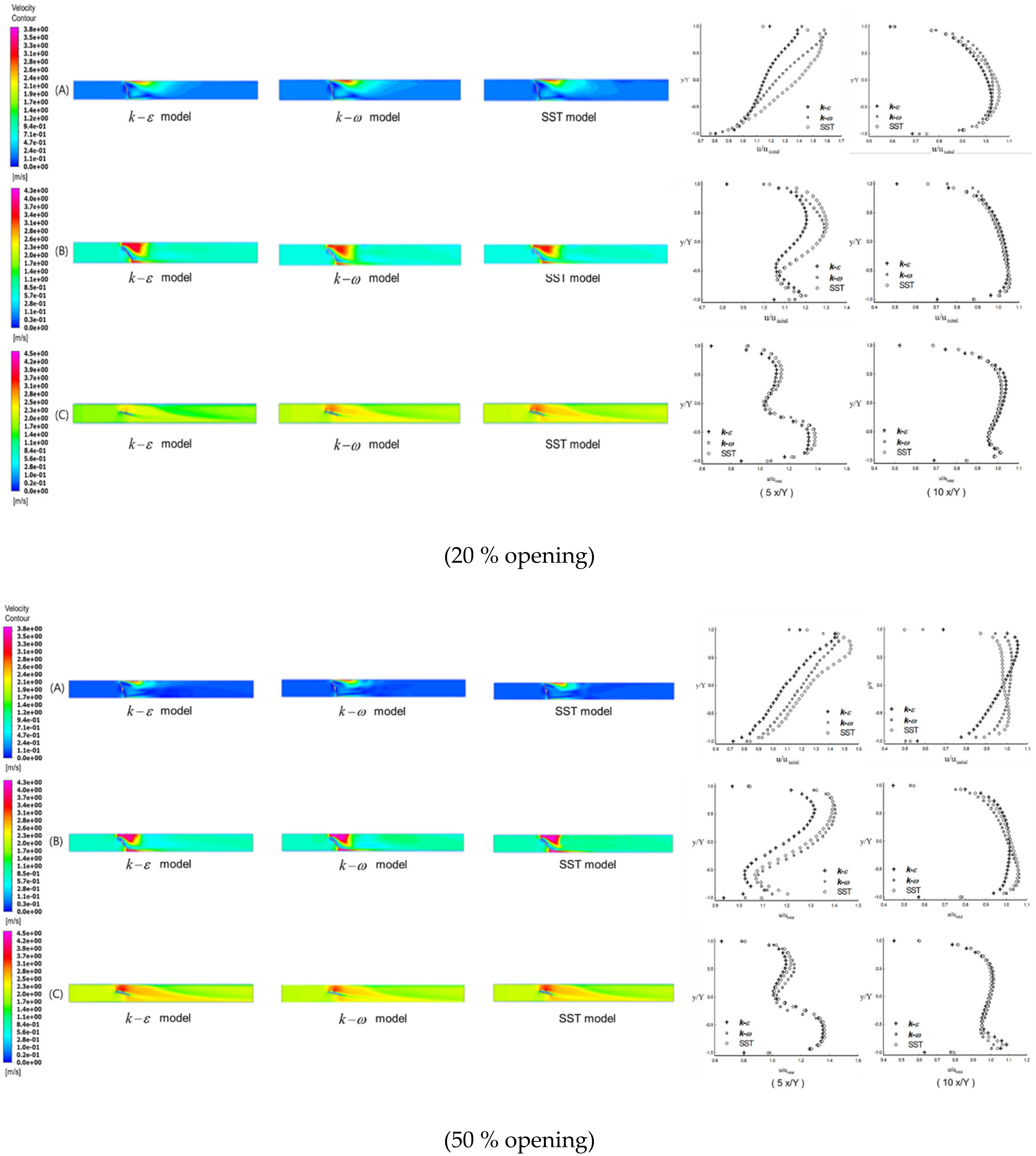
- Higher turbulence due to vortices was observed for the k − ω model expressed with higher turbulence kinetic energy, followed by the SST and models. The difference between the results of turbulence models increased with decreasing valve size and disc opening. This can be attributed to the increasing turbulence effect which could cause lots of discrepancies between turbulence models, especially in areas with large pressure drop and sharp velocity increase.
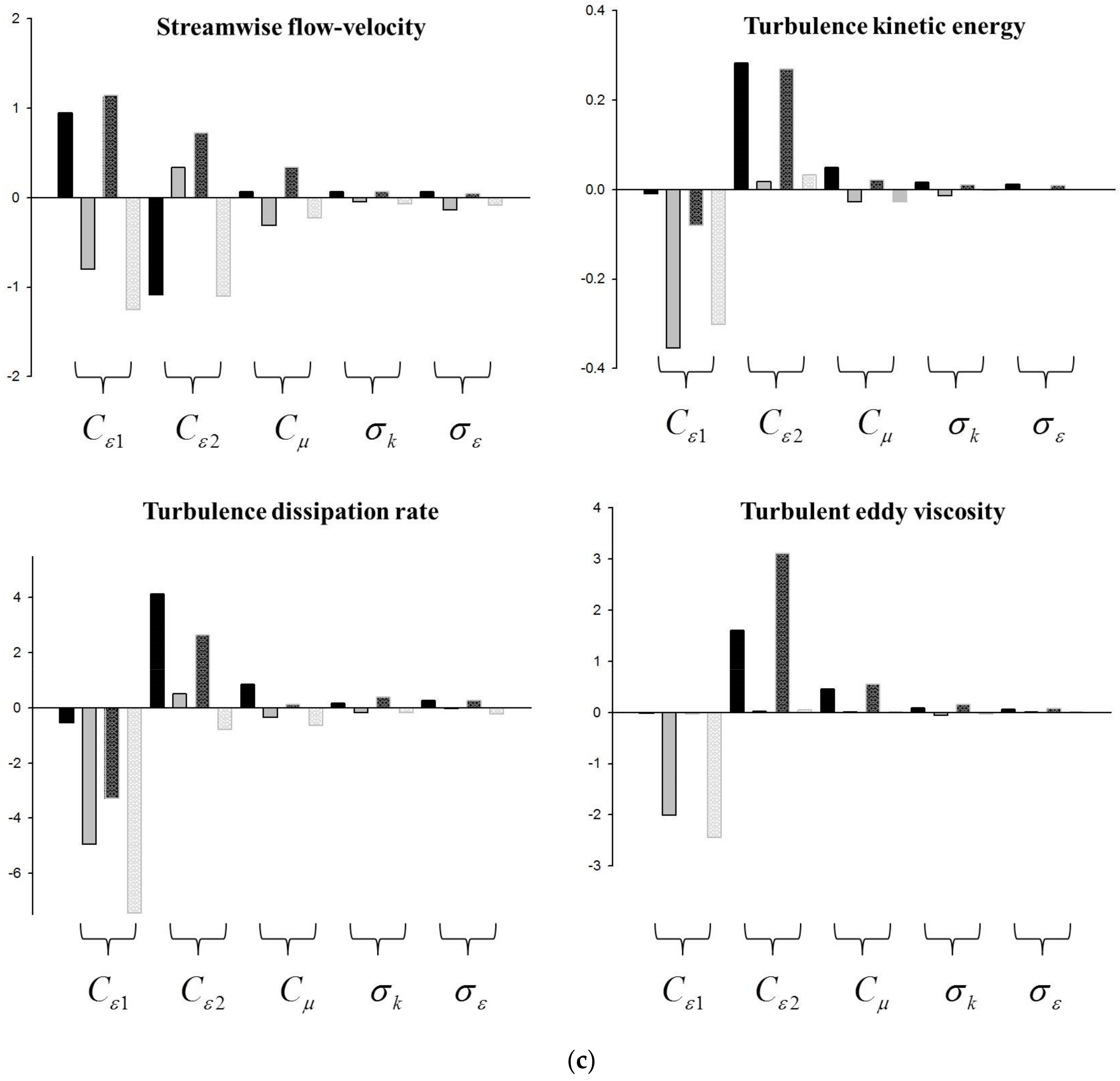
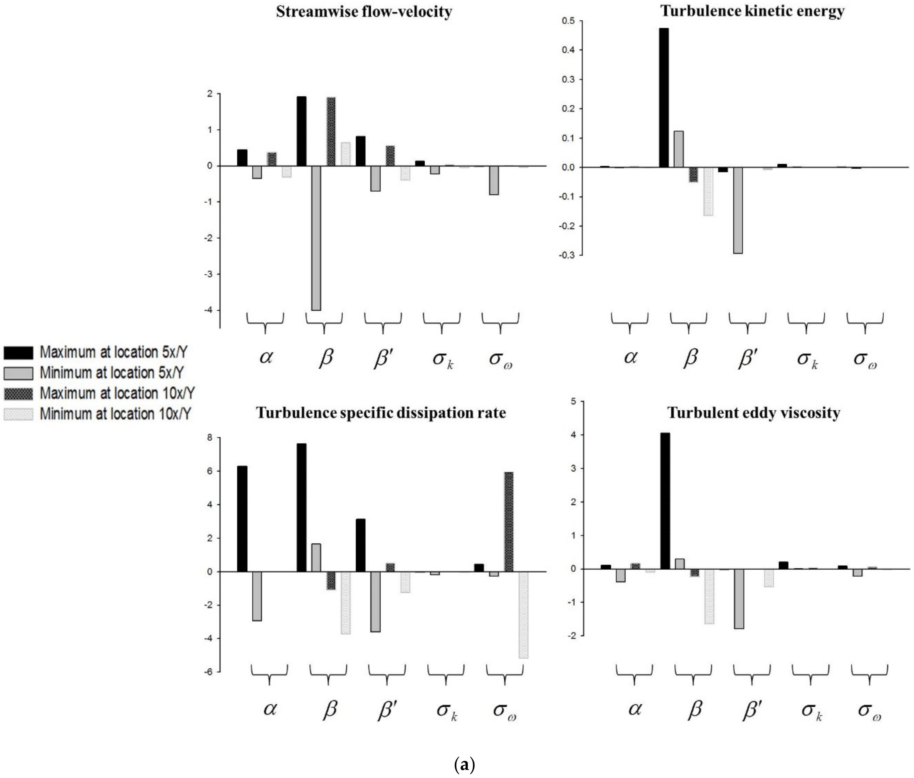
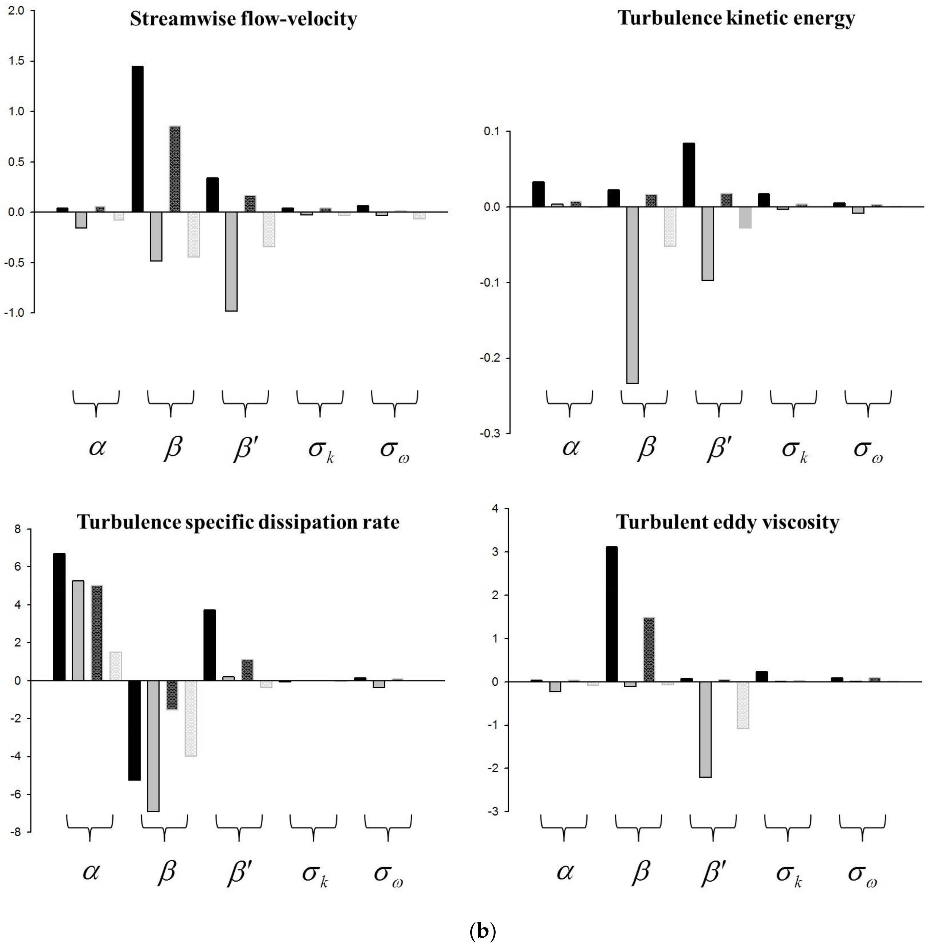
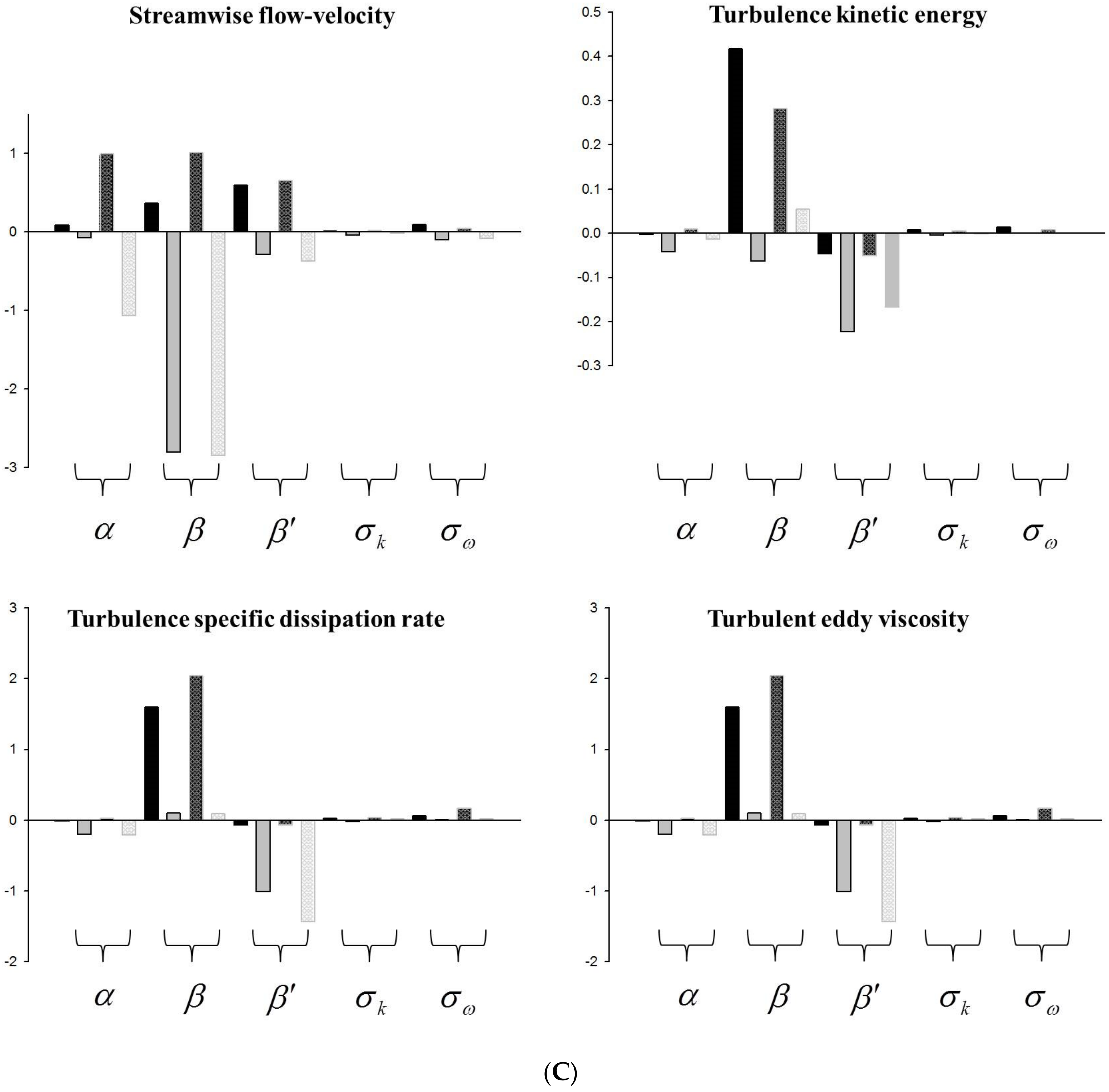
- The most sensitive flow property was turbulence dissipation rate and this property was mainly affected by the values of constants of and for the , k − ω turbulence model, and by the values of constants of , partly by constant of for the k − ω turbulence model.
- For the k − ω turbulence model, relatively smaller value of sensitivity with different locations and openings were observed compared to the turbulence model. From sensitivity analysis results, it can be suggested that turbulence constant adoptability in numerical calculations should be checked when using each turbulence model.
- For the numerical calculations, currently three turbulence models were the most frequently used turbulent models. These models were advantageous over other turbulence models because the computational conditions could be easily implemented. Therefore, the investigated analysis will be helpful to current users of turbulence models. The results of this research could also be widely applied to engineering design using the various valve systems.
- The numerical approach presented in this paper can be effectively used in future research on various valve flow analyses especially for the cavitation phenomenon.
Author Contributions
Funding
Institutional Review Board Statement
Informed Consent Statement
Data Availability Statement
Acknowledgments
Conflicts of Interest
Nomenclature
| Eddy viscosity constant | |
| Wall distance | |
| , , | Turbulence constant |
| Cross-diffusion in the model | |
| Flow coefficient of the valve | |
| Blending function | |
| Auxiliary function | |
| Wall damping function | |
| Specific gravity of the fluid | |
| Turbulence kinetic energy | |
| Turbulence mixing length | |
| Constant in the valve flow coefficient | |
| P | Turbulence production |
| Q | Flow rate |
| Turbulence Reynolds number | |
| Mean velocity strain-rate tensor | |
| Sensitivity coefficient | |
| t | Time |
| Mean average velocity | |
| Flow velocity parallel to the wall | |
| , | Examined constants in sensitivity analysis |
| Wall function | |
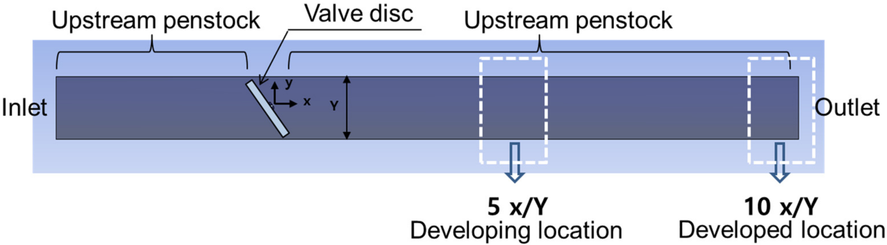
| x/Y | Specific location (x: distance from the valve, Y; nominal valve size) |
| y/Y | Specific location (y: height, Y; nominal valve size) |
| Increment of turbulence constant | |
| Pressure drop across the valve | |
| Greek Symbols | |
| Turbulence Reynolds stress | |
| Kronecker delta tensor | |
| Dynamic viscosity | |
| Turbulence eddy viscosity | |
| Turbulence dissipation rate | |
| Specific turbulent dissipation rate | |
| Vorticity | |
| Density of the material | |
| Ratio of specific heat | |
| , | Explicit wall term |
| , | Turbulence constant |
| , | Turbulence constant |
| , , | Turbulence constant |
References
- Kaartinen, N.H.; Juhala, P.J. Fluid Flow Control Device. U.S. Patent No. 4,258,740, 31 March 1981. [Google Scholar]
- Smith, P.; Zappe, R.W. Valve Selection Handbook: Engineering Fundamentals for Selecting the Right Valve Design for Every Industrial Flow Application; Elsevier: Amsterdam, The Netherlands, 2004. [Google Scholar]
- American Water Works Association. Problem Organisms in Water; American Water Works Association: Denver, CO, USA, 2004. [Google Scholar]
- Del Toro, A.; Johnson, M.C.; Spall, R.E. Computational fluid dynamics investigation of butterfly valve performance factors. J. Am. Water Work. Assoc. 2015, 107, E243–E254. [Google Scholar] [CrossRef]
- Lin, F.; Schohl, G. CFD Prediction and Validation of Butterfly Valve Hydrodynamic Forces. In Critical Transitions in Water and Environmental Resources Management; American Society of Civil Engineers: Reston, VA, USA, 2004; pp. 1–8. [Google Scholar]
- Song, X.; Wang, L.; Park, Y. Fluid and Structural Analysis of Large Butterfly Valve. In AIP Conference Proceedings; American Institute of Physics: College Park, MD, USA, 2008; pp. 311–314. [Google Scholar]
- Guan Song, X.; Park, Y. Numerical Analysis of Butterfly Valve-Prediction of Flow Coefficient and Hydrodynamic Torque Coefficient. In Proceedings of the World Congress on Engineering and Computer Science, San Francisco, CA, USA, 24–26 October 2007; pp. 24–26. [Google Scholar]
- Henderson, A.D.; Sargison, J.E.; Walker, G.J.; Haynes, J. A numerical prediction of the hydrodynamic torque acting on a safety butterfly valve in a hydro-electric power scheme. WSEAS Trans. Fluid Mech. 2008, 1, 218. [Google Scholar]
- Huang, C.; Kim, R. Three-dimensional analysis of partially open butterfly valve flows. J. Fluids Eng. 1996, 118, 562–568. [Google Scholar] [CrossRef]
- Blevins, R. Applied Fluid Dynamics Handbook; Van Nostrand Reinhold Co.: New York, NY, USA, 1984. [Google Scholar]
- Davis, J.; Stewart, M. Predicting globe control valve performance—Part I: CFD modeling. J. Fluids Eng. 2002, 124, 772–777. [Google Scholar] [CrossRef]
- Chern, M.; Wang, C. Control of volumetric flow-rate of ball valve using V-port. J. Fluids Eng. 2004, 126, 471–481. [Google Scholar] [CrossRef]
- Hinz, D.; Kim, T.; Fried, E. Statistics of the Navier–Stokes-alpha-beta regularization model for fluid turbulence. J. Phys. A Math. Theor. 2014, 47, 055501. [Google Scholar] [CrossRef][Green Version]
- Thalabard, S.; Nazarenko, S.; Galtier, S.; Medvedev, S. Anomalous spectral laws in differential models of turbulence. J. Phys. A Math. Theor. 2015, 48, 285501. [Google Scholar] [CrossRef][Green Version]
- Rigola, J.; Aljure, D.; Lehmkuhl, O.; Perez-Segarra, C.D.; Oliva, A. Numerical Analysis of the Turbulent Fluid Flow Through Valves. Geometrical Aspects Influence at Different Positions. In IOP Conference Series: Materials Science and Engineering; IOP Publishing: Bristol, UK, 2015; p. 012026. [Google Scholar]
- Zhang, S.C.; Zhang, Y.L.; Fang, Z.M. Numerical simulation and analysis of ball valve three-dimensional flow based on CFD. In IOP Conference Series: Earth and Environmental Science; IOP Publishing: Bristol, UK, 2012; p. 052024. [Google Scholar]
- Leutwyler, Z.; Dalton, C. A computational study of torque and forces due to compressible flow on a butterfly valve disk in mid-stroke position. J. Fluids Eng. 2006, 128, 1074–1082. [Google Scholar] [CrossRef]
- Said, M.M.; Abdelmeguid, H.; Rabie, L. The Accuracy Degree of CFD Turbulence Models for Butterfly Valve Flow Coefficient Prediction. Am. J. Ind. Eng. 2016, 4, 14–20. [Google Scholar]
- Wu, X.; Wallace, J.; Hickey, J. Boundary layer turbulence and freestream turbulence interface, turbulent spot and freestream turbulence interface, laminar boundary layer and freestream turbulence interface. Phys. Fluids 2019, 31, 045104. [Google Scholar] [CrossRef]
- Sharma, M.; Verma, M.; Chakraborty, S. Anisotropic energy transfers in rapidly rotating turbulence. Phys. Fluids 2019, 31, 085117. [Google Scholar] [CrossRef]
- Li, H.; Yang, Z. Separated boundary layer transition under pressure gradient in the presence of free-stream turbulence. Phys. Fluids 2019, 31, 104106. [Google Scholar]
- Wilcox, D. Comparison of two-equation turbulence models for boundary layers with pressure gradient. AIAA J. 1993, 31, 1414–1421. [Google Scholar] [CrossRef]
- Wilcox, D. Turbulence Modeling for CFD; DCW industries: La Canada, CA, USA, 1998. [Google Scholar]
- Jones, W.P.; Launder, B. The prediction of laminarization with a two-equation model of turbulence. Int. J. Heat Mass Transf. 1972, 15, 301–314. [Google Scholar] [CrossRef]
- Launder, B.; Sharma, B. Application of the energy-dissipation model of turbulence to the calculation of flow near a spinning disc. Lett. Heat Mass Transf. 1974, 1, 131–137. [Google Scholar] [CrossRef]
- Pletcher, R.; Tannehill, J.; Anderson, D. Computational Fluid Mechanics and Heat Transfer; CRC Press: Boca Raton, FL, USA, 2012. [Google Scholar]
- Bottema, M. Turbulence closure model constants and the problems of inactive atmospheric turbulence. J. Wind. Eng. Ind. Aerodyn. 1997, 67, 897–908. [Google Scholar] [CrossRef]
- Comte-Bellot, G.; Corrsin, S. The use of a contraction to improve the isotropy of grid-generated turbulence. J. Fluid Mech. 1966, 25, 657–682. [Google Scholar] [CrossRef]
- Hrenya, C.M.; Bolio, E.J.; Chakrabarti, D.; Sinclair, J.L. Comparison of low Reynolds number k − ε turbulence models in predicting fully developed pipe flow. Chem. Eng. Sci. 1995, 50, 1923–1941. [Google Scholar] [CrossRef]
- Launder, B.; Spalding, D. The numerical computation of turbulent flows. In Numerical prediction of flow, heat transfer, turbulence and combustion. Pergamon 1983, 96–116. [Google Scholar] [CrossRef]
- Launder, B.E.; Spalding, D.B. Lectures in Mathematical Models of Turbulence; Academic Press: New York, NY, USA, 1972. [Google Scholar]
- Shih, T.H. An improved k-epsilon model for near-wall turbulence and comparison with direct numerical simulation. NASA STI Recon Tech. Rep. N 1990, 90, 27983. [Google Scholar]
- Sarkar, A.; So, R.M.C. A critical evaluation of near-wall two-equation models against direct numerical simulation data. Int. J. Heat Fluid. Flow. 1997, 18, 197–208. [Google Scholar] [CrossRef]
- Chen, Y.-S.; Kim, S.-W. Computation of Turbulent Flows Using an Extended k-Epsilon Turbulence Closure Model; NASA CR-179204; Universities Space Research Association: Columbia, MD, USA; Science and Engineering Directorate: Ottawa, ON, Canada, 1987. [Google Scholar]
- Sarkar, T.; Sayer, P.G.; Fraser, S.M. Flow simulation past axisymmetric bodies using four different turbulence models. Appl. Math. Model. 1997, 21, 783–792. [Google Scholar] [CrossRef]
- Shih, T.-H.; Liou, W.W.; Shabbir, A.; Yang, Z.; Zhu, J. A new k-ϵ eddy viscosity model for high reynolds number turbulent flows. Comput. Fluids 1995, 24, 227–238. [Google Scholar] [CrossRef]
- Błazik-Borowa, E. The analysis of the channel flow sensitivity to the parameters of the k–ε method. Int. J. Numer. Methods Fluids 2008, 58, 1257–1286. [Google Scholar] [CrossRef]
- Benton, J.; Kalitzin, G.; Gould, A. Application of two-equation turbulence models in aircraft design. In Proceedings of the 34th Aerospace Sciences Meeting and Exhibit, Reno, NV, USA, 15–18 January 1996; p. 327. [Google Scholar]
- Wilcox, D.C. Formulation of the kw turbulence model revisited. AIAA J. 2008, 46, 2823–2838. [Google Scholar] [CrossRef]
- Huang, P.G.; Bardina, J.; Coakley, T. Turbulence modeling validation, testing, and development. NASA Tech. Memo. 1997, 110446, 147. [Google Scholar]
- Kok, J.C. Resolving the dependence on freestream values for the k-turbulence model. AIAA J. 2000, 38, 1292–1295. [Google Scholar] [CrossRef]
- Kim, M.-S.; Ryu, J.-H.; Oh, S.-J.; Yang, J.-H.; Choi, S.-W. Numerical Investigation on Influence of Gas and Turbulence Model for Type III Hydrogen Tank under Discharge Condition. Energies 2020, 13, 6432. [Google Scholar] [CrossRef]
- Menter, F.; Ferreira, J.C.; Esch, T.; Konno, B. The SST Turbulence Model with Improved Wall Treatment for Heat Transfer Predictions in Gas Turbines. In Proceedings of the International Gas Turbine Congress, Tokyo, Japan, 2–7 November 2003. [Google Scholar]
- Williams, S.; Trembley, J.; Miller, J.P. Flow Monitoring using Flow Control Device. U.S. Patent No. 7,092,797, 15 August 2006. [Google Scholar]
- ISA. Standard, Control Valve Sizing Equations for Compressible Fluids, ISA-S75; The International Society of Automation: Research Triangle Park, NC, USA, 2007. [Google Scholar]
- ISA. Standard, Control Valve Capacity Test Procedures, ISA-S75; The International Society of Automation: Research Triangle Park, NC, USA, 2007. [Google Scholar]
- Hutchison, J. ISA Handbook of Control Valves: A Comprehensive Reference Book Containing Application and Design Information; Instrument Society of America: Research Triangle Park, NC, USA, 1976. [Google Scholar]
- Sandalci, M.; Mancuhan, E.; Alpman, E.; Kucukada, K. Effect of the flow conditions and valve size on butterfly valve performance. J. Therm. Sci. Technol. 2010, 3, 103–112. [Google Scholar]
- Nazary, H.; Aalipour, N.; Alizadeh, M. Investigation of the Flow and Cavitation in a Butterfly Calve. J. Mech. Res. Appl. 2011, 3, 37–47. [Google Scholar]
- Kim, C.K.; Yoon, J.Y.; Shin, M.S. Experimental study for flow characteristics and performance evaluation of butterfly valves. In IOP Conference Series: Earth and Environmental Science; IOP Publishing: Bristol, UK, 2010; p. 012098. [Google Scholar]
- ANSYS, Inc. ANSYS CFX-Solver Modeling Guide; Release 12.0; ANSYS, Inc.: Canonsburg, PA, USA, 2009; Volume 15, pp. 162–168. [Google Scholar]
- Blocken, B.; Gualtieri, C. Ten iterative steps for model development and evaluation applied to Computational Fluid Dynamics for Environmental Fluid Mechanics. Environ. Model. Softw. 2012, 33, 1–22. [Google Scholar] [CrossRef]
- Patel, Y. Numerical Investigation of Flow Past a Circular Cylinder and in a Staggered Tube Bundle Using Various Turbulence Models. Master’s Thesis, Lappeenranta University of Technology, Faculty of Technology, Lappeenranta, Finland, 24 August 2010. [Google Scholar]
- Błazik-Borowa, E. The application example of the sensitivity analysis of the solution to coefficients of the k-ε model. Budownictwo i Architektura 2012, 10, 53–68. [Google Scholar] [CrossRef]
- Colin, E.; Etienne, S.; Pelletier, D.; Borggaard, J. Application of a sensitivity equation method to turbulent flows with heat transfer. Int. J. Therm. Sci. 2005, 44, 1024–1038. [Google Scholar] [CrossRef]


Publisher’s Note: MDPI stays neutral with regard to jurisdictional claims in published maps and institutional affiliations. |
© 2021 by the authors. Licensee MDPI, Basel, Switzerland. This article is an open access article distributed under the terms and conditions of the Creative Commons Attribution (CC BY) license (https://creativecommons.org/licenses/by/4.0/).
Share and Cite
Choi, S.-W.; Seo, H.-S.; Kim, H.-S. Analysis of Flow Characteristics and Effects of Turbulence Models for the Butterfly Valve. Appl. Sci. 2021, 11, 6319. https://doi.org/10.3390/app11146319
Choi S-W, Seo H-S, Kim H-S. Analysis of Flow Characteristics and Effects of Turbulence Models for the Butterfly Valve. Applied Sciences. 2021; 11(14):6319. https://doi.org/10.3390/app11146319
Chicago/Turabian StyleChoi, Sung-Woong, Hyoung-Seock Seo, and Han-Sang Kim. 2021. "Analysis of Flow Characteristics and Effects of Turbulence Models for the Butterfly Valve" Applied Sciences 11, no. 14: 6319. https://doi.org/10.3390/app11146319
APA StyleChoi, S.-W., Seo, H.-S., & Kim, H.-S. (2021). Analysis of Flow Characteristics and Effects of Turbulence Models for the Butterfly Valve. Applied Sciences, 11(14), 6319. https://doi.org/10.3390/app11146319