Voice Activation for Low-Resource Languages

Abstract

Voice activation systems are used to find a pre-defined word or phrase in the audio stream. Industry solutions, such as “OK, Google” for Android devices, are trained with millions of samples. In this work, we propose and investigate several ways to train a voice activation system when the in-domain data set is small. We compare self-training exemplar pre-training, fine-tuning a model pre-trained on another domain, joint training on both an out-of-domain high-resource and a target low-resource data set, and unsupervised pre-training. In our experiments, the unsupervised pre-training and the joint-training with a high-resource data set from another domain significantly outperform a strong baseline of fine-tuning a model trained on another data set. We obtain 7–25% relative improvement depending on the model architecture. Additionally, we improve the best test accuracy on the Lithuanian data set from 90.77% to 93.85%.

1. Introduction

Many modern devices are equipped with voice control. Still, high-quality speech recognition requires many computational resources, which means that a voice-controlled device needs a network connection to remote servers to perform recognition. On the other hand, it is not practical to stream all the audio to the remote servers, both due to privacy and network usage reasons.

That is why some voice-controlled devices (e.g., Android-powered mobile phones) use voice activation before actual speech recognition. A voice activation system is a system that detects a pre-defined keyword or key phrase (e.g., “OK, Google”) in the audio stream. The problem of creating a high-quality voice activation system (or a keyword spotting system) with low resource consumption is heavily investigated by both research and industry [1]. Low resource consumption is dictated by the use of embedded devices. For example, Google researchers presented their work about a server-side automatic speech recognition model that uses 58 million trainable parameters [2], and a keyword spotter model that uses 300–350 thousand parameters [3]. The problem of general speech recognition is more complex than the problem of finding a pre-defined keyword, but still the voice activation system must be fast, robust to noise and speech perturbations and accurate with a very limited amount of computational resources. This makes the problem of building high-quality voice activation quite challenging.

Voice-activation systems find their applications in various areas. For example, it can be used to detect sensitive terms in telephone tapping and audio monitoring device recordings for easier crime analysis [4]. Another example is speeding up the command transmission for the aerospace field [5]. Voice activation is widely used for triggering voice control in personal voice assistants [6].

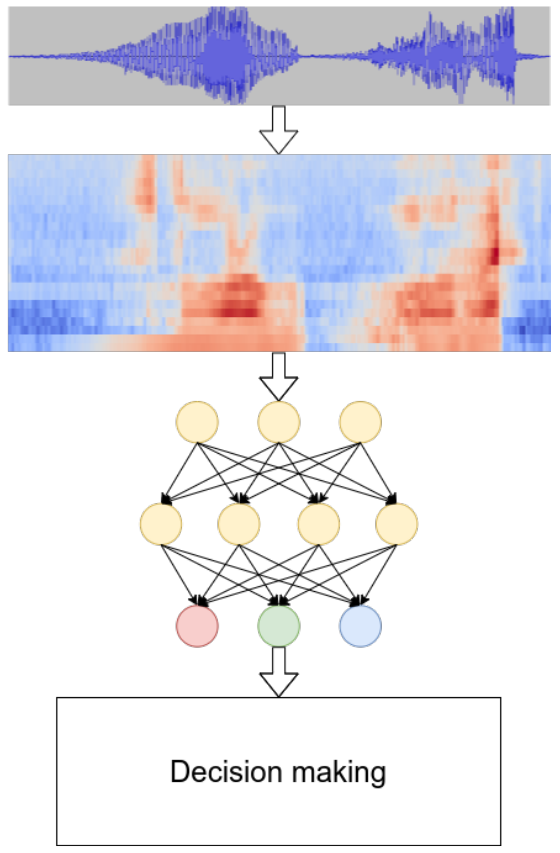
The majority of modern voice activation systems consist of the following parts (see Figure 1 for illustration):

• Acoustic feature extraction.
• Acoustic model.
• Decision-making model.

In the first part, the acoustic features are extracted from the source audio. Typically, it is done by segmenting the audio in short, possibly overlapping, frames, then computing the features in each frame. Many research studies have used log-mel filterbanks [7,8,9,10,11].

The acoustic model is used to compute the probability of some acoustic event, given the observed audio. There are several popular choices for acoustic events: phonemes [6,12,13] and words [14,15] are widely used. Usually, this module is the most resource demanding in the voice activation system.

Finally, the decision-making module is used to choose between several options: whether there is a keyword in the processed audio segment and if so, which one it is. This module can be quite complicated, especially in the case of phoneme-based spotters [16]. In the case of using the whole keywords as acoustic events, the decision-making module is usually just comparing the resulting probabilities with a threshold.

Historically, voice activation systems were based on hidden Markov models [17] or pattern matching approaches, such as dynamic time wrapping [18]. However, since 1990, top-performing voice activation systems have been using (almost exclusively) neural networks as an acoustic model [16,19,20,21,22].

Neural networks are powerful approximators and widely used in many areas. One of the drawbacks of using neural networks is that in many cases, a large labeled data set is needed to train such a model. For example, the authors of [16] use hundreds of thousands of samples per keyword and the authors or [23] use millions.

However, in some cases, it is not practical or even hardly possible to collect a large data set. In the case of designing a voice activation system for custom, user-defined keywords, it might hurt the user experience if it is necessary to repeat the custom keyword many times before real usage. Another example is quickly adapting the system to a new sensitive keyword in the aforementioned crime analysis application. Creating a voice activation system for low-resource languages, such as Lithuanian or Latvian, could be another example when the effective use of a small data set is needed, because it is difficult to find enough native speakers for creating a large audio database.

In this work, we investigate several known and new ways to improve the quality of a voice activation system on a low-resource labeled data set, comparing to the standard supervised way of acoustic model training. We use a small Lithuanian data set [24] in order to compare the investigated methods. In all our experiments, we use the same neural network architecture but introduce some changes to audio features (Section 3.4.1), use different kinds of pre-training (Section 3.4.2 and Section 3.4.3) or modify the training procedure (Section 3.4.4 and Section 3.4.5).

2. Related Works

This work concerns the problem of training a highly accurate voice activation system in a low-resource data set setup. This problem is tackled in several related works, most often connected to work with low-resourced languages.

One of the most productive ideas is to use a bigger out-of-domain data set in one way or another. For instance, the authors of [25] use an English corpus to improve the quality of keyword spotter for the under-resourced Luganda corpus. The authors use a neural network trained as an autoencoder in two scenarios:

• The neural network accepts audio features as input and is trained to output the same audio features.
• The neural network accepts audio features as input and is trained to output the audio features of another audio file, but with same keyword as that in the input file.

In both scenarios, the intermediate layers of neural network have fewer neurons than the number of audio features. This helps to build bottleneck features (the activation of neurons of intermediate levels), which hopefully contain useful information about the audio signal and less noise than the original audio features. In the second scenario, the additional property is achieved: the information about non-keyword traits (such as the gender of the speaker, the speed of pronunciation, and so on) is not necessary for the optimal model (because the model predicts the audio features of another pronunciation of the same keyword). The research studies show, experimentally, that the resulting features are better than popular mel-frequency cepstral coefficients. The neural networks are trained on relatively small data sets (still at least 10 times bigger than the setup in this work). The extracted features are used for the voice activation system, which is trained on the data sets with a size comparable to the size of the data set used in this work. The use of multilingual data is related to the methods of this research, but our setup is a bit simpler (we train the whole model on multiple data sets, not only the feature extractor, which means that the training procedure is the same for both pre-training and training, and only the data sets are different). Additionally, for some of our proposed methods, there is no need for a relatively big annotated data set in the target domain.

The authors of [26] present another example of the use of multilingual data for extracting the bottleneck features. The researchers train tandem acoustic modeling for phone recognition of several languages and use bottleneck features of this model as acoustic features for speech recognition as well as keyword spotting for a low-resource target language. This idea is extended in [27] for the pre-training of hybrid speech recognition systems. The authors of [28] propose to create phone mapping between languages (namely, English and Spanish in their experiments) in order to transfer a model pre-trained on a big data set for use on a smaller data set in another language. Comparing to these methods, the methods that are investigated in our work do not require phone transcription for a corpus used for pre-training and do not require the existence of phone mapping between languages.

An entirely different way to improve the quality of a keyword spotter in a low-resource setup is to generate synthetic data and use it in training. The authors of [29] use a model pre-trained on 200 million 2-second audio clips in order to extract bottleneck features. This extractor is used to train a result keyword spotter on a small data set augmented with samples generated with speech synthesis. The authors show that synthetic data are enough to build a high-quality keyword spotter, if the pre-trained feature extractor is good enough. Unfortunately good speech synthesis might not be available for some languages.

Another method is to pre-train the model in an unsupervised manner. In such a way, the pre-training data set can be unlabeled, which hopefully makes it easier to obtain. A very successful way of unsupervised pre-training for automatic speech recognition is proposed in [30]. The authors use a large unlabeled audio corpus to train a model that predicts audio features from the audio features of neighboring frames (similar to a language modeling task). The features extracted from this “language model” are experimentally very useful for speech recognition, even for very small data sets (1 h of labeled speech, compared to hundreds of hours of a typical speech recognition data set). Several researchers propose to use a similar method for voice activation problem with limited data sets [31,32]. We use the results of [31] as one of the baselines for our methods. Some disadvantage of this method might be a possibly heavy feature extractor for use in a low-resource consumption setup.

Many methods have been proposed to apply deep learning in a low-resource data set setup for other problems, specifically for speech recognition and image classification. In our work, we try to adapt some of these methods for the voice activation problem.

Unsupervised pre-training [33] is an example of a general framework, which can be applied when the in-domain labeled data set is small, but there is a possibility to get a bigger unlabeled data set. In an unsupervised pre-training scenario, the model is trained on a large corpus of data without target labels (possibly on some artificial problem) and then the model parameters are used to initialize training on the target data set. Such pre-training can be used in speech recognition [34].

A popular way of pre-training for image classification is proposed in [35]. The authors choose several seed images without labels, generate many other samples from the chosen images by using augmentations, and pre-train the classifier on this data set. The original seed image and the images generated from it form a classifer for a pre-training classification problem. The classifier trained on this task shows good results on the downstream problem. To the best of our knowledge, our work is the first attempt to adapt this pre-training method to a keyword-spotting task.

Semisupervised learning and, specifically, self-training is another method to improve the quality of a resulting model [36,37] by using unlabeled data. The general framework of self-training is as follows:

• Train a model on a small labeled data set.
• Use the current model to label bigger unlabeled data set.
• Form a new data set with newly labeled samples by applying the augmentations to the input features, but leaving the target labels as predicted on the uncorrupted samples.
• Uptrain the model from the previous step on both the original data set and the samples from the new data set.
• Repeat steps 2–4 until the quality is no longer improved.

In this work, we try to apply the method proposed in [37] for speech recognition for a voice activation problem (see Section 3.4.4 for more details).

3. Experiments

In this section, we investigate some existing and some new methods for training a voice activation system in a low-resource data set setup. In Section 3.1, the used data sets are described. In Section 3.2, we describe the neural network architectures used. The training procedure and the description of the used hyperparameters are given in Section 3.3. Finally, Section 3.4 contains the description of all investigated methods and the resulting metrics. For the result discussion, see Section 4.

3.1. Data Sets

We used the following two data sets in our experiments:

• Lithuanian data set—a small data set for experiments in a low-resource setup [24].
• English data set—Google Speech Commands [38], used for multilingual experiments.

The Google Speech Commands data set [38] was released in August 2017 under a Creative Common license. The data set contains around 100,000 one-second-long utterances of 30 short words by thousands of different people, as well as background noise samples, such as pink noise, white noise, and human-made sounds. As in [38], in our classification task, we discriminate between 12 classes: 10 short words, an unknown word and a silence class.

The Lithuanian data set [24] was collected in a similar fashion [31]. This data set consists of one-second recordings of 28 people, each of them uttering 20 words on a mobile phone. Background noised were recorded on the same devices. The whole data set contains 781 samples. As in [31], in our classification task, we discriminate between 15 classes: 13 words, an unknown word and a silence class.

3.2. Neural Network Architectures

For all our experiments, we use two types of neural network architectures:

• Feedforward (ff) neural network with three fully-connected layers and ReLU activation.
• Residual convolutional neural networks with different number of layers (res8, res15, res26) and possibly reduced number of feature maps in convolutions (res8-narrow res15-narrow, res26-narrow).

These models are chosen because they represent a fairly strong baseline for a voice activation system [15] and allow us to directly compare our results with [31] on the Lithuanian data set [24]. We encourage the reader to see works [15,31] for more detailed description of these architectures; here, we give a short summary.

ff models accept the audio features, have three fully connected layers with 128, 64 and C neurons, respectively, where C is a number of target classes. The first two layers have ReLU activation and the last one has softmax activation. The scheme of the ff neural network is illustrated in Figure 2.

Residual networks use residual connections to allow a stable gradient path in a neural network with a high number of layers. The basic building block of networks that we use in this work is a residual block. Its scheme is presented in Figure 3. Each residual block has two $3\times 3$ convolutional layers with ReLU activation. Batch normalization is used for the activation of these layers. The output of such a residual block is equal to the sum of the block’s input and the batch normalized activation of the second convolutional layer.

We use the same types of residual neural networks as in [15,31]. They consist of the following:

• Bias-free $3\times 3$ convolutional layer.
• Optional average pooling layer (e.g., $4\times 3$ layer in res8).
• Several residual blocks (see Figure 3).
• $3\times 3$ convolutional layer.
• Batch normalization layer.
• Average pooling layer.
• Fully-connected layer of size C, where C is the number of classes to discriminate.
• Softmax layer.

All the layers are zero-padded. For some variants, dilated convolutions are applied to increase the receptive field of the model. The scheme of the res8 model is presented in Figure 4.

We use the same notation and parameters as in [31]. The parameters used for residual neural network variants are specified in

Table 1. Parameters of ResNet architectures used in the experiments. The names follow [15,31].

Architecture Name	Residual Blocks	Feature Maps	Average Pooling	Dilation
res8	3	45	$(4\times 3)$	no
res8-narrow	3	19	$(4\times 3)$	no
res15	6	45	no	yes
res15-narrow	6	19	no	yes
res26	12	45	$(2\times 2)$	no
res26-narrow	12	19	$(2\times 2)$	no

.

For all our experiments (except for wav2vec, see Section 3.4.1) log-mel filterbanks with 25 ms frame width, 10 ms frame shift and 80 bins [31] are used.

3.3. Training Procedure

Our experiments for the English data set follow the same procedure as the TensorFlow reference for the Google Speech Commands data set [38]. The data set is split into training (80% of the total number of samples), validation (10%), and test (10%) sets. For the Lithuanian data set, we follow the procedure from [31]: 326 records for training, 75 for validation, 88 for testing (the rest of the samples are background noise samples). At the train stage, background noise is added to a training sample with a probability of $P_n$. We use a stochastic gradient descent for optimization with initial learning rate L, momentum M and batch size B. At each S step, the validation accuracy is computed. If the value is not improved, the best checkpoint is reloaded, and the learning rate is divided by $L^{\prime }$. The training for each experiment is stopped after 6 learning rate drops. Finally, the test accuracy is computed. We run each experiment three times and report the average test accuracy. The distributions and values for a random hyperparameter search can be seen in

Table 2. Distributions for a random hyperparameter search.

Value	Distribution
$P_n$	$0.7$
$-{log}_{10}L$	$U\{0,3\}$
M	$0.9$
${log}_{2}B$	$U\{4,7\}$
${log}_{2}S$	$U\{3,12\}$
$L^{\prime }$	$U\{1.1,10.0\}$

(U is a uniform or discrete uniform distribution).

3.4. Methods

For each experiment, a random hyperparameter search is conducted (see Section 3.3 for more details) and the best models on the validation set is chosen. Note that we report only the test accuracy (averaged over three runs) for all the methods. For more discussion of the results, see Section 4.

3.4.1. Baseline

We use the results from [31] as the baseline results for our work. In that work, the authors trained models on the following acoustic features:

• Log-mel filterbanks (the same setup as in Section 3.3).
• Acoustic features extracted with wav2vec [30] encoder.

The wav2vec encoder is trained in a unsupervised manner on a huge unlabeled English data set. The authors of [31] showed that using such features helps to improve the accuracy of the voice activation system on a small data set, such as that which we use in our experiments. The resulting test accuracies for both feature pipelines and different neural network architectures are presented in

Table 3. Test accuracy for log-mel filterbanks and wav2vec feature pipelines [31]. The best result for each architecture is highlighted.

Architecture	Log-Mel Filterbanks	Wav2vec [31]
ff	72.31%	78.46%
res8-narrow	73.85%	84.62%
res8	78.46%	90.77%
res15-narrow	83.08%	80.00%
res15	89.23%	86.15%
res26-narrow	83.08%	72.31%
res26	80.00%	83.08%

.

In the following sections, we propose and investigate several methods to achieve even better detection quality, using only a small Lithuanian data set [24] and, possibly, some other labeled and unlabeled out-of-domain data.

3.4.2. Fine-Tuning of Pre-Trained Model

Fine-tuning the model, which was pre-trained on a large data set, is a popular way to improve model performance in a specific domain or task [39,40]. This method is widely used in computer vision problems [41,42], but also can be used in voice-related problems, e.g., speech recognition [43].

The general framework is as follows:

• Train the classifier on a bigger dataset with a random weights initialization.
• Uptrain the classifier on the target data set.

The general idea is that the classifier can learn implicit features on a bigger data set, which can be useful for a target data set, even though the pre-training data set may be out of the domain. Sometimes, some parameters must be changed before the uptraining, e.g., if the target and original data sets have a different number of classes. In that case, at least the final fully-connected layer in our models must be reinitialized.

We use the Google Speech Commands data set [38] for pre-training. The log-mel filterbanks are chosen as input features. The hyperparameter grid search is conducted for three model architectures and the best performing models are chosen for the fine-tuning. The training procedure is explained in Section 3.3. The test accuracy on the Google Speech Commands data set [38] is presented in

Table 4. Test accuracy for models pre-trained on the Google Speech Commands data set [38].

Architecture	Accuracy
res8	96.29%
res15	95.45%
res26-narrow	95.93%

for the selected models.

After that, we train neural networks on the Lithuanian data set following the procedure from Section 3.3, but we initialize the weights using the pre-trained models except for the final linear layer, which is initialized randomly. We also do a hyperparameter grid search; the resulting metrics for the best models are presented in

Table 5. The test accuracy after the fine-tuning on the target data set. The best result for each architecture is highlighted.

Architecture	Baseline Accuracy	Method Accuracy
res8	78.46%	89.23%
res15	89.23%	90.77%
res26-narrow	83.08%	89.23%

.

3.4.3. Exemplar-Like Pre-Training

The kind of pre-training discussed in this subsection is based on the pre-training suggested in [35] for image classification. We propose to adapt this method for a voice activation problem. The authors of [35] proposed to learn (in unsupervised manner) features that are invariant to some predefined transformations in the following way:

• Select n “interesting” (seed) samples.
• Generate $k-1$ samples from each of the samples using the augmentations (so we have a data set of $nk$ samples): the source sample and $k-1$ augmented samples form a surrogate class.
• Train a classifier to distinguish n surrogate classes.

The resulting classifier can be fine-tuned to the downstream task. “Interesting” samples means that the chosen sample should contain information similar to the samples of the downstream task. For example, the authors of [35] chose patches of images with a considerable gradient so these patches contain objects or parts of objects.

Carefully chosen augmentations should ensure that the resulting classifier are invariant for some transformations. For example, in [35] scaling, translation and rotation are used so the classifier does not depend on the position of the classified object, just on the object itself.

We use two kinds of augmentations: the common for the Google Speech Commands data set [38] described in Section 3.3 and SpecAugment [44]. The latter consists of a combination of the following transformations (for the detailed explanation see [44]):

• Time wrapping.
• Frequency masking.
• Time masking.

The severity of the transformations are controlled via a set of hyperparameters. The values used in our experiments are presented in

Table 6. Hyperparameter values for the used SpecAugment levels.

Parameter/Level	1	2	3
Maximal number of frames in frequency mask	25	15	40
Maximal number of frequencies in time mask	25	15	40
Number of frequency masks	1	2	1
Number of time masks	1	2	1

.

The level of SpecAugment transformations is a hyperparameter in all the grid searches in this subsection.

We conduct two sets of experiments using this kind of pre-training. First, we run our best baseline classifier (res8 trained on wav2vec features) on the 20 h of lectures in Lithuanian. More specifically, we apply our classifier to one-second patches of each audio file with 100 ms shift between the patches. After that, we select the top K patches by the model score for each of the classes. We make sure that no two patches are closer than 10 s apart (so that we do not have too similar samples). Those patches are the seed samples for the first set of experiments. We try several values of K, so the numbers of seed samples are 100, 1000 and 2000. After that, we conduct a grid search for several architectures. The resulting metrics of the pre-training are presented in

Table 7. Test accuracy of the pre-trained classifiers on surrogate samples.

Architecture	Seed Samples	SpecAugment Level	Accuracy
res8	100	1	96.00%
res8	100	2	100.00%
res8	100	3	99.00%
res8	1000	3	97.00%
res15	2000	1	92.40%
res15	2000	3	90.00%
res8	2000	2	97.10%

(only models with testing accuracy equal or higher than 90% were left).

The weights of these models are used for initialization (except for the last linear layer) for fine-tuning on the target Lithuanian data set. The choice of model is one of the hyperparameters in the grid search. The results are presented in

Table 8. Resulting test accuracy after the pre-training on the surrogate samples. The best result for each architecture is highlighted.

Architecture	Baseline Accuracy	Method Accuracy
res8	78.46%	80.00%
res15	89.23%	81.54%

.

The second set of experiments is the same as the first, except for the choice of the seed samples. There, we choose to use 200 audio files from the training set of the target data set as a source of samples for the surrogate classes. We hypothesize that pre-training on the samples from the target domain will improve the quality of the resulting classifier. The results of the pre-training are presented in

Table 9. Test accuracy of the classifiers pre-trained on the training set of the Lithuanian data set.

Architecture	SpecAugment Level	Accuracy
res15	1	38.92%
res15	2	79.77%
res15	3	67.48%
res26-narrow	1	72.22%
res26-narrow	2	5.76%
res26-narrow	3	22.79%
res8	1	1.28%
res8	2	83.48%
res8	3	82.33%

. The pre-training metrics are quite poor, as we are not able to get even 10% accuracy for some choices of architecture and SpecAugment levels. Still, even the 1.28% that we obtain for res8 and the 1st level is better than a random guess ($\frac{1}{200}=0.5\%$). We think that the results are worse than in Table 7 because the seed samples in this set of experiments are much closer to one another, some because of the same speaker, some because of the same spoken word.

As in the first set of experiments, we fine-tune the resulting models on the target data set. The results are presented in

Table 10. Resulting test accuracy after the pre-training on the training set of the Lithuanian data set. The best result for each architecture is highlighted.

Architecture	Baseline Accuracy	Method Accuracy
res8	78.46%	75.38%
res15	89.23%	90.77%
res26-narrow	83.08%	75.38%

.

3.4.4. Self-Training

Self-training is the method of semi-supervised training when the baseline (teacher) model is used to label the available unlabeled data [36]. These labels are called pseudolabels. The samples with pseudolabels are appended to the supervised data, and the target (student) model is trained on the resulting data set. The expected profit comes from the fact that the student model learns to obtain the same results on the augmented (corrupted) samples as the teacher model on the original (not corrupted) samples. Self-training shows good results for speech recognition [37].

We use the same set of lectures as in Section 3.4.3 for obtaining the unlabeled data. We use baseline models to obtain the top 1000 samples for each class by the model score, making sure that all samples are not closer than 10 s to one another. All the samples with pseudolabels are added only to the training set. The validation set and test set remain the same in order to make a fair comparison with the baseline models. The choice of the baseline model for pseudolabels generation is a hyperparameter in a grid search in this experiment. The results are presented in

Table 11. Test accuracy after the training with the initial data set and added samples with pseudolabels. The best result for each architecture is highlighted.

Architecture	Baseline Accuracy	Method Accuracy
ff	72.31%	63.08%
res8-narrow	73.85%	75.38%
res8	78.46%	81.54%
res15-narrow	83.08%	84.62%
res15	89.23%	86.15%
res26-narrow	83.08%	58.46%
res26	80.00%	81.54%

.

3.4.5. Joint Training on Two Languages

A good classifier should be invariant to some transformations. It might be difficult to learn these patterns in low-resource settings. Using a bigger annotated data set could help with this problem.

We conduct a set of experiments on using the Google Speech Commands data set [38] in order to make a better classifier for the Lithuanian data set. First, we add all the samples from the bigger data set to the Lithuanian data set as unknown samples and train the classifier on the resulting data set. The results are presented in

Table 12. Test accuracy after using the Google Speech Commands data set [38] as additional unknown samples. The best result for each architecture is highlighted.

Architecture	Baseline Accuracy	Method Accuracy
ff	72.31%	66.15%
res8-narrow	73.85%	67.69%
res8	78.46%	76.92%
res15-narrow	83.08%	80.00%
res15	89.23%	80.00%
res26-narrow	83.08%	55.38%
res26	80.00%	76.92%

.

Next, we train the classifiers with the task to distinguish both target words from the Google Speech Commands data set [38] and the Lithuanian data set. The results are in

Table 13. Test accuracy on both Lithuanian and English commands after using Google Speech Commands dataset [38] as additional target samples.

Architecture	Accuracy
ff	93.01%
res15	97.85%
res15-narrow	97.67%
res26	97.31%
res26-narrow	94.98%
res8	96.77%
res8-narrow	96.06%

and

Table 14. Test accuracy on Lithuanian commands after using Google Speech Commands data set [38] as additional target samples. The best result for each architecture is highlighted.

Architecture	Baseline Accuracy	Method Accuracy
ff	72.31%	33.33%
res8-narrow	73.85%	19.44%
res8	78.46%	47.22%
res15-narrow	83.08%	20.83%
res15	89.23%	62.50%
res26-narrow	83.08%	19.44%
res26	80.00%	54.17%

.

Finally, we repeat the previous experiment but repeat every Lithuanian sample in the training set T times in order for the samples of different languages to make a comparable influence on the training process. $T=10$ show the best results, which are presented in

Table 15. Test accuracy after using Google Speech Commands data set [38] as additional target samples with repeating each Lithuanian sample 10 times. The best result for each architecture is highlighted.

Architecture	Baseline Accuracy	Method Accuracy
ff	72.31%	84.62%
res8-narrow	73.85%	89.23%
res8	78.46%	84.62%
res15-narrow	83.08%	89.23%
res15	89.23%	93.85%
res26-narrow	83.08%	90.77%
res26	80.00%	90.77%

.

4. Discussion

The results of all our experiments are summarized in

Table 16. Test accuracy from the experiments of this work. The results that are better than the log-mel filterbanks baseline are highlighted.

Method/Architecture	ff	res8-narrow	res8	res15-narrow	res15	res26-narrow	res26
Section 3.4.1
Log-mel filterbanks	72.31%	73.85%	78.46%	83.08%	89.23%	83.08%	80.00%
wav2vec [31]	78.46%	84.62%	90.77%	80.00%	86.15%	72.31%	83.08%
Section 3.4.2
Fine-tuning	N/A	N/A	89.23%	N/A	90.77%	89.23%	N/A
Section 3.4.3
Exemplar on surrogate	N/A	N/A	80.00%	N/A	81.54%	N/A	N/A
Exemplar on trainset	N/A	N/A	75.38%	N/A	90.77%	75.38%	N/A
Section 3.4.4
Self-training	63.08%	75.38%	81.54%	84.62%	86.15%	58.46%	81.54%
Section 3.4.5
GSC as unknown	66.15%	67.69%	76.92%	80.00%	80.00%	55.38%	76.92%
Added GSC	33.33%	19.44%	47.22%	20.83%	62.50%	18.44%	54.17%
Added GSC with scale	84.62%	89.23%	84.62%	89.23%	93.85%	90.77%	90.77%

. For each architecture and for each investigated method, we show the test accuracy of the best model (models are chosen by their performance on the validation set). As you can see, there are several ways to improve the baseline quality of voice activation in a low-resource setup.

The goal of our research is to find methods of improving the detection quality of a voice activation system in a low-resource data set setup, comparing to standard training on the data set in a supervised manner (log-mel filterbanks baseline from Section 3.4.1).

Using unsupervised pre-trained audio features is one such way, as was discussed in [31]. Fine-tuning a model, which was pre-trained on a similar data set but in another language improves the results as expected.

The exemplar-like pre-training [35] on surrogate audio patches produces comparable results to the baseline, but is unable to get a significant margin. We think that it is because our chosen augmentations do not cause invariance to the change of a speaker, which is crucial for voice activation. We also try to pre-train the model on the target training set itself, and obtain some improvement for some models, but a quality loss for others.

Self-training also helps, especially for the models with a lower capacity. Still, using wav2vec is almost always better. We think that it is because of not very useful data sets for pseudo-labels generation: there is no actual pronunciation for more than half of the target words in our lecture data set. It is not just an experiment drawback, but also a practical limitation: it is difficult to find a good source data set for pseudo-labels if the target words are rare. In other cases, we think that the investigation of iterative pseudo-labeling [45] might be an interesting choice for future research.

Finally, we try to use the Google Speech Commands data set [38] in the training process itself, not only as a pre-training dataset. We hope that adding the data set as unknown samples will help the classifier to learn more patterns, but there is no success. Making English commands an additional target helps the resulting classifier, but the results on only Lithuanian commands are horrible. We find out that it is because the Lithuanian part of the data set is small, compared to the Google Speech Commands part, so it is favorable for the classifier to focus on the English part. After that, we scale up the Lithuanian part by simply repeating the samples several times. The resulting metrics are better than the log-mel filterbanks baseline in all models and better than the wav2vec baseline in all models except res8.

The accuracy is not the best metric for assessing the detection quality of a voice activation system because it does not reflect the balance between the two different types of errors [1]:

• False alarms.
• False rejects.

Many researchers and practitioners use a false alarm rate (the rate of false detections over the samples without a keyword) and false reject rate (the rate of skipping the detection over the samples with a keyword). Still, the researchers that use the Google Speech Commands data set [38] (and collected with the same principles Lithuanian dataset [24]) use the test accuracy as a final metric (see, for example, [15,46,47]) because it is easier to compare in the case of many keywords, and because a relatively big and diverse speech data set is required in order to get a reasonable estimate for a false alarm rate.

Still, it is possible to compute the false alarm rate and the false reject rate, even for a multiclass models. The obvious method is to compute these metrics for each keyword, but for our experiments it is not very practical: each keyword has a handful of test samples. Additionally, comparing two models by 15 pairs of false alarm rates and false reject rates is not a trivial task. Because of that, we use the same method as proposed in scikit-learn tutorials [48]: we convert this multiclass problem to a binary classification. For a sample with a target label t out of n classes with predicted probabilities $p_1,\dots ,p_n$ we consider $n-1$ negative samples with predicted probabilities $p_1,\dots ,p_{t-1},p_t,\dots ,p_n$ and one positive sample with a predicted probability $p_t$. 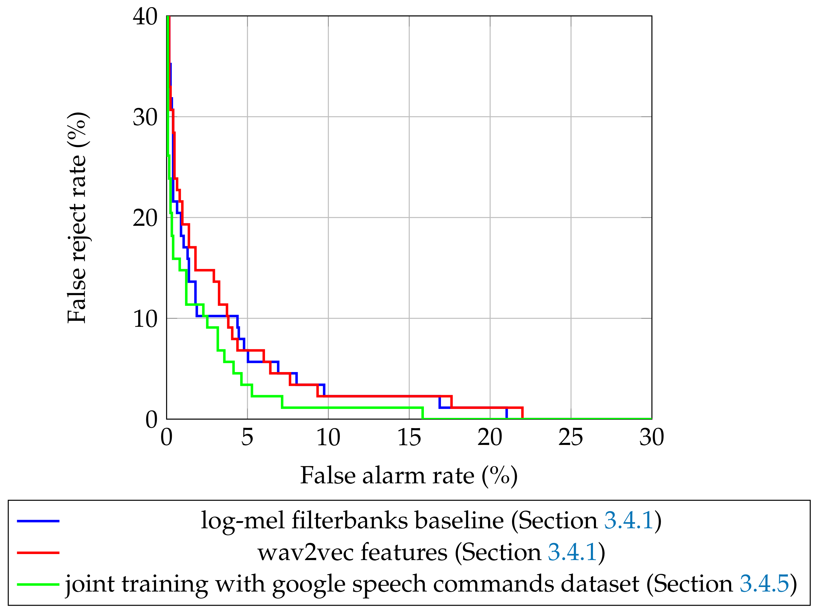After that, we can compute false alarm rate and false reject rate. The values of these metrics for different values of classifying thresholds are presented in Figure 5 for the best models for baseline methods and joint training (Section 3.4.5).

As you can see, the model with the highest quality (trained with joint training on both data sets) is almost everywhere better than all the competitors, which supports our findings. It is interesting to see that, though the wav2vec model is better than the log-mel filterbanks one in terms of accuracy, it is significantly worse in operating points, with a low false alarm rate. The equal error rate (EER, the minimal value that both false alarm rate and false reject rate can accept at the same time for a some value of threshold) also shows that the best log-mel filterbanks model ($\mathrm{ERR}=5.68\%$) can be better than a wav2vec ($\mathrm{ERR}=5.84\%$) for some scenarios. The best model from the proposed joint training method has an equal error rate $4.5\%$.

5. Conclusions

In this work, we investigated several ways to improve the voice activation system quality in a low-resource language setup. The experiments on the Lithuanian data set [31] showed that the use of unsupervised pre-trained audio features and joint training with a bigger annotated data set could beat a popular baseline of fine-tuning the model trained on a high-resource data set. For example, in our experiments, the proposed joint training on the Lithuanian [31] and Google Speech Commands data sets [38] showed a relative improvement from 7% (ff-model) to 25% (res26-narrow model) for the Lithuanian part of the test-set, compared to a simple fine-tuning. In addition, we improved the best test accuracy on the Lithuanian data set across all architectures to 93.85% from 90.77%, reported in [31].

In future works, the combinations of investigated methods could be researched. Additionally, better augmentations causing speaker invariance can be studied in order to improve the quality of exemplar-like pre-training.

References

1. Kolesau, A.; Šešok, D. Voice Activation Systems for Embedded Devices: Systematic Literature Review. Informatica 2020, 31, 65–88. [Google Scholar] [CrossRef] [Green Version]
2. Alon, U.; Pundak, G.; Sainath, T.N. Contextual Speech Recognition with Difficult Negative Training Examples. In Proceedings of the ICASSP 2019—2019 IEEE International Conference on Acoustics, Speech and Signal Processing (ICASSP), Brighton, UK, 12–17 May 2019; pp. 6440–6444. [Google Scholar] [CrossRef] [Green Version]
3. Rybakov, O.; Kononenko, N.; Subrahmanya, N.; Visontai, M.; Laurenzo, S. Streaming Keyword Spotting on Mobile Devices. In Proceedings of the Interspeech 2020, 21st Annual Conference of the International SpeechCommunication Association, Virtual Event, Shanghai, China, 25–29 October 2020; Meng, H., Xu, B., Zheng, T.F., Eds.; ISCA: Baixas, France, 2020; pp. 2277–2281. [Google Scholar] [CrossRef]
4. Kavya, H.P.; Karjigi, V. Sensitive keyword spotting for crime analysis. In Proceedings of the 2014 IEEE National Conference on Communication, Signal Processing and Networking (NCCSN), Palakkad, India, 10–12 October 2014; pp. 1–6. [Google Scholar] [CrossRef]
5. Tabibian, S. A voice command detection system for aerospace applications. Int. J. Speech Technol. 2017, 20, 1049–1061. [Google Scholar] [CrossRef]
6. Gruenstein, A.; Alvarez, R.; Thornton, C.; Ghodrat, M. A Cascade Architecture for Keyword Spotting on Mobile Devices. arXiv 2017, arXiv:1712.03603. [Google Scholar]
7. Liu, H.; Abhyankar, A.; Mishchenko, Y.; Sénéchal, T.; Fu, G.; Kulis, B.; Stein, N.D.; Shah, A.; Vitaladevuni, S.N.P. Metadata-Aware End-to-End Keyword Spotting. In Proceedings of the Interspeech 2020, 21st Annual Conference of the International Speech Communication Association, Virtual Event, Shanghai, China, 25–29 October 2020; Meng, H., Xu, B., Zheng, T.F., Eds.; ISCA: Baixas, France, 2020; pp. 2282–2286. [Google Scholar] [CrossRef]
8. Wu, H.; Jia, Y.; Nie, Y.; Li, M. Domain Aware Training for Far-Field Small-Footprint Keyword Spotting. In Proceedings of the Interspeech 2020, 21st Annual Conference of the International Speech Communication Association, Virtual Event, Shanghai, China, 25–29 October 2020; Meng, H., Xu, B., Zheng, T.F., Eds.; ISCA: Baixas, France, 2020; pp. 2562–2566. [Google Scholar] [CrossRef]
9. Zhang, K.; Wu, Z.; Yuan, D.; Luan, J.; Jia, J.; Meng, H.; Song, B. Re-Weighted Interval Loss for Handling Data Imbalance Problem of End-to-End Keyword Spotting. In Proceedings of the Interspeech 2020, 21st Annual Conference of the International Speech Communication Association, Virtual Event, Shanghai, China, 25–29 October 2020; Meng, H., Xu, B., Zheng, T.F., Eds.; ISCA: Baixas, France, 2020; pp. 2567–2571. [Google Scholar] [CrossRef]
10. Zhang, P.; Zhang, X. Deep Template Matching for Small-Footprint and Configurable Keyword Spotting. In Proceedings of the Interspeech 2020, 21st Annual Conference of the International Speech Communication Association, Virtual Event, Shanghai, China, 25–29 October 2020; Meng, H., Xu, B., Zheng, T.F., Eds.; ISCA: Baixas, France, 2020; pp. 2572–2576. [Google Scholar] [CrossRef]
11. Lopatka, K.; Bocklet, T. State Sequence Pooling Training of Acoustic Models for Keyword Spotting. In Proceedings of the Interspeech 2020, 21st Annual Conference of the International Speech Communication Association, Virtual Event, Shanghai, China, 25–29 October 2020; Meng, H., Xu, B., Zheng, T.F., Eds.; ISCA: Baixas, France, 2020; pp. 4338–4342. [Google Scholar] [CrossRef]
12. Kumatani, K.; Panchapagesan, S.; Wu, M.; Kim, M.; Strom, N.; Tiwari, G.; Mandal, A. Direct modeling of raw audio with DNNS for wake word detection. In Proceedings of the 2017 IEEE Automatic Speech Recognition and Understanding Workshop, ASRU 2017, Okinawa, Japan, 16–20 December 2017; pp. 252–257. [Google Scholar] [CrossRef]
13. Myer, S.; Tomar, V.S. Efficient Keyword Spotting Using Time Delay Neural Networks. In Proceedings of the Interspeech 2018, 19th Annual Conference of the International Speech Communication Association, Hyderabad, India, 2–6 September 2018; Yegnanarayana, B., Ed.; ISCA: Baixas, France, 2018; pp. 1264–1268. [Google Scholar] [CrossRef] [Green Version]
14. Manor, E.; Greenberg, S. Voice trigger system using fuzzy logic. In Proceedings of the 2017 International Conference on Circuits, System and Simulation (ICCSS), London, UK, 14–17 July 2017; pp. 113–118. [Google Scholar] [CrossRef]
15. Tang, R.; Lin, J. Deep Residual Learning for Small-Footprint Keyword Spotting. In Proceedings of the 2018 IEEE International Conference on Acoustics, Speech and Signal Processing (ICASSP), Calgary, AB, Canada, 15–20 April 2018; pp. 5484–5488. [Google Scholar] [CrossRef] [Green Version]
16. Chen, G.; Parada, C.; Heigold, G. Small-footprint keyword spotting using deep neural networks. In Proceedings of the 2014 IEEE International Conference on Acoustics, Speech and Signal Processing (ICASSP), Florence, Italy, 4–9 May 2014; pp. 4087–4091. [Google Scholar]
17. Rohlicek, J.R.; Russell, W.; Roukos, S.; Gish, H. Continuous hidden Markov modeling for speaker-independent word spotting. In Proceedings of the International Conference on Acoustics, Speech, and Signal Processing, Glasgow, UK, 23–26 May 1989; Volume 1, pp. 627–630. [Google Scholar] [CrossRef]
18. Zeppenfeld, T.; Waibel, A.H. A hybrid neural network, dynamic programming word spotter. In Proceedings of the ICASSP-92: 1992 IEEE International Conference on Acoustics, Speech, and Signal Processing, San Francisco, CA, USA, 23–26 May 1992; Volume 2, pp. 77–80. [Google Scholar] [CrossRef]
19. Morgan, D.P.; Scofield, C.L.; Lorenzo, T.M.; Real, E.C.; Loconto, D.P. A keyword spotter which incorporates neural networks for secondary processing. In Proceedings of the International Conference on Acoustics, Speech, and Signal Processing, Albuquerque, NM, USA, 3–6 April 1990; Volume 1, pp. 113–116. [Google Scholar] [CrossRef]
20. Morgan, D.P.; Scofield, C.L.; Adcock, J.E. Multiple neural network topologies applied to keyword spotting. In Proceedings of the ICASSP 91: 1991 International Conference on Acoustics, Speech, and Signal Processing, Toronto, ON, Canada, 14–17 April 1991; Volume 1, pp. 313–316. [Google Scholar] [CrossRef]
21. Naylor, J.A.; Huang, W.Y.; Nguyen, M.; Li, K.P. The application of neural networks to wordspotting. In Proceedings of the 1992 Conference Record of the Twenty-Sixth Asilomar Conference on Signals, Systems Computers, Pacific Grove, CA, USA, 26–28 October 1992; Volume 2, pp. 1081–1085. [Google Scholar] [CrossRef]
22. Wu, M.; Panchapagesan, S.; Sun, M.; Gu, J.; Thomas, R.; Vitaladevuni, S.N.P.; Hoffmeister, B.; Mandal, A. Monophone-Based Background Modeling for Two-Stage On-Device Wake Word Detection. In Proceedings of the 2018 IEEE International Conference on Acoustics, Speech and Signal Processing, ICASSP 2018, Calgary, AB, Canada, 15–20 April 2018; pp. 5494–5498. [Google Scholar] [CrossRef]
23. Jose, C.; Mishchenko, Y.; Sénéchal, T.; Shah, A.; Escott, A.; Vitaladevuni, S.N.P. Accurate Detection of Wake Word Start and End Using a CNN. In Proceedings of the Interspeech 2020, 21st Annual Conference of the International Speech Communication Association, Virtual Event, Shanghai, China, 25–29 October 2020; Meng, H., Xu, B., Zheng, T.F., Eds.; ISCA: Baixas, France, 2020; pp. 3346–3350. [Google Scholar] [CrossRef]
24. Kolesau, A.; Šešok, D. Lithuanian Speech Commands Dataset. Available online: https://github.com/kolesov93/lt_speech_commands (accessed on 4 May 2021).
25. Menon, R.; Kamper, H.; van der Westhuizen, E.; Quinn, J.; Niesler, T. Feature Exploration for Almost Zero-Resource ASR-Free Keyword Spotting Using a Multilingual Bottleneck Extractor and Correspondence Autoencoders. arXiv 2019, arXiv:1811.08284. [Google Scholar]
26. Knill, K.; Gales, M.; Ragni, A.; Rath, S. Language independent and unsupervised acoustic models for speech recognition and keyword spotting. In Proceedings of the Annual Conference of the International Speech Communication Association, INTERSPEECH, Singapore, 14–18 September 2014; pp. 16–20. [Google Scholar]
27. Wang, H.; Ragni, A.; Gales, M.J.F.; Knill, K.M.; Woodland, P.C.; Zhang, C. Joint decoding of tandem and hybrid systems for improved keyword spotting on low resource languages. In Proceedings of the INTERSPEECH 2015, 16th Annual Conference of the International Speech Communication Association, Dresden, Germany, 6–10 September 2015; ISCA: Baixas, France, 2015; pp. 3660–3664. [Google Scholar]
28. Tetariy, E.; Bar-Yosef, Y.; Silber-Varod, V.; Gishri, M.; Alon-Lavi, R.; Aharonson, V.; Opher, I.; Moyal, A. Cross-language phoneme mapping for phonetic search keyword spotting in continuous speech of under-resourced languages. Artif. Intell. Res. 2015, 4, 72–82. [Google Scholar] [CrossRef]
29. Lin, J.; Kilgour, K.; Roblek, D.; Sharifi, M. Training Keyword Spotters with Limited and Synthesized Speech Data. In Proceedings of the ICASSP 2020—2020 IEEE International Conference on Acoustics, Speech and Signal Processing (ICASSP), Barcelona, Spain, 4–8 May 2020; pp. 7474–7478. [Google Scholar] [CrossRef] [Green Version]
30. Schneider, S.; Baevski, A.; Collobert, R.; Auli, M. wav2vec: Unsupervised Pre-Training for Speech Recognition. Proc. Interspeech 2019, 2019, 3465–3469. [Google Scholar] [CrossRef] [Green Version]
31. Kolesau, A.; Šešok, D. Unsupervised Pre-Training for Voice Activation. Appl. Sci. 2020, 10, 8463. [Google Scholar] [CrossRef]
32. Seo, D.; Oh, H.S.; Jung, Y. Wav2KWS: Transfer Learning From Speech Representations for Keyword Spotting. IEEE Access 2021, 9, 80682–80691. [Google Scholar] [CrossRef]
33. Erhan, D.; Bengio, Y.; Courville, A.; Manzagol, P.A.; Vincent, P.; Bengio, S. Why Does Unsupervised Pre-training Help Deep Learning? J. Mach. Learn. Res. 2010, 11, 625–660. [Google Scholar] [CrossRef]
34. Hinton, G.; Deng, L.; Yu, D.; Dahl, G.; Mohamed, A.R.; Jaitly, N.; Senior, A.; Vanhoucke, V.; Nguyen, P.; Kingsbury, B.; et al. Deep Neural Networks for Acoustic Modeling in Speech Recognition. IEEE Signal Process. Mag. 2012, 29, 82–97. [Google Scholar] [CrossRef]
35. Dosovitskiy, A.; Springenberg, J.; Riedmiller, M.; Brox, T. Discriminative Unsupervised Feature Learning with Exemplar Convolutional Neural Networks. IEEE Trans. Pattern Anal. Mach. Intell. 2014, 1. [Google Scholar] [CrossRef] [PubMed] [Green Version]
36. Triguero, I.; García, S.; Herrera, F. Self-labeled techniques for semi-supervised learning: Taxonomy, software and empirical study. Knowl. Inf. Syst. 2015, 42. [Google Scholar] [CrossRef]
37. Kahn, J.; Lee, A.; Hannun, A. Self-Training for End-to-End Speech Recognition. In Proceedings of the ICASSP 2020—2020 IEEE International Conference on Acoustics, Speech and Signal Processing (ICASSP), Barcelona, Spain, 4–8 May 2020; pp. 7084–7088. [Google Scholar] [CrossRef] [Green Version]
38. Warden, P. Speech Commands: A Dataset for Limited-Vocabulary Speech Recognition. arXiv 2018, arXiv:1804.03209. [Google Scholar]
39. Li, H.; Chaudhari, P.; Yang, H.; Lam, M.; Ravichandran, A.; Bhotika, R.; Soatto, S. Rethinking the Hyperparameters for Fine-tuning. In Proceedings of the International Conference on Learning Representations, Addis Ababa, Ethiopia, 26–30 April 2020. [Google Scholar]
40. Ge, W.; Yu, Y. Borrowing Treasures From the Wealthy: Deep Transfer Learning Through Selective Joint Fine-Tuning. In Proceedings of the IEEE Conference on Computer Vision and Pattern Recognition (CVPR), Honolulu, HI, USA, 21–26 July 2017. [Google Scholar]
41. Chen, L.; Papandreou, G.; Kokkinos, I.; Murphy, K.; Yuille, A.L. DeepLab: Semantic Image Segmentation with Deep Convolutional Nets, Atrous Convolution, and Fully Connected CRFs. IEEE Trans. Pattern Anal. Mach. Intell. 2018, 40, 834–848. [Google Scholar] [CrossRef] [PubMed]
42. Ren, S.; He, K.; Girshick, R.; Sun, J. Faster R-CNN: Towards Real-Time Object Detection with Region Proposal Networks. In Advances in Neural Information Processing Systems; Cortes, C., Lawrence, N., Lee, D., Sugiyama, M., Garnett, R., Eds.; Curran Associates, Inc.: Red Hook, NY, USA, 2015; Volume 28. [Google Scholar]
43. Bansal, S.; Kamper, H.; Livescu, K.; Lopez, A.; Goldwater, S. Pre-training on high-resource speech recognition improves low-resource speech-to-text translation. In Proceedings of the 2019 Conference of the North American Chapter of the Association for Computational Linguistics: Human Language Technologies, Volume 1 (Long and Short Papers), Minneapolis, MN, USA, 6–11 June 2021; Association for Computational Linguistics: Minneapolis, MN, USA, 2019; pp. 58–68. [Google Scholar] [CrossRef]
44. Park, D.S.; Chan, W.; Zhang, Y.; Chiu, C.C.; Zoph, B.; Cubuk, E.D.; Le, Q.V. SpecAugment: A Simple Data Augmentation Method for Automatic Speech Recognition. Proc. Interspeech 2019, 2019, 2613–2617. [Google Scholar] [CrossRef] [Green Version]
45. Xu, Q.; Likhomanenko, T.; Kahn, J.; Hannun, A.; Synnaeve, G.; Collobert, R. Iterative Pseudo-Labeling for Speech Recognition. In Proceedings of the Interspeech 2020, 21st Annual Conference of the International Speech Communication Association, Virtual Event, Shanghai, China, 25–29 October 2020; Meng, H., Xu, B., Zheng, T.F., Eds.; ISCA: Baixas, France, 2020; pp. 1006–1010. [Google Scholar] [CrossRef]
46. Li, X.; Wei, X.; Qin, X. Small-Footprint Keyword Spotting with Multi-Scale Temporal Convolution. In Proceedings of the Interspeech 2020, 21st Annual Conference of the International Speech Communication Association, Virtual Event, Shanghai, China, 25–29 October 2020; Meng, H., Xu, B., Zheng, T.F., Eds.; ISCA: Baixas, France, 2020; pp. 1987–1991. [Google Scholar] [CrossRef]
47. Mo, T.; Yu, Y.; Salameh, M.; Niu, D.; Jui, S. Neural Architecture Search for Keyword Spotting. In Proceedings of the Interspeech 2020, 21st Annual Conference of the International Speech Communication Association, Virtual Event, Shanghai, China, 25–29 October 2020; Meng, H., Xu, B., Zheng, T.F., Eds.; ISCA: Baixas, France, 2020; pp. 1982–1986. [Google Scholar] [CrossRef]
48. Pedregosa, F.; Varoquaux, G.; Gramfort, A.; Michel, V.; Thirion, B.; Grisel, O.; Blondel, M.; Prettenhofer, P.; Weiss, R.; Dubourg, V.; et al. Scikit-learn: Machine Learning in Python. J. Mach. Learn. Res. 2011, 12, 2825–2830. [Google Scholar]
Figure 1. The scheme of a typical voice activation system.
Applsci 11 06298 g001
Figure 2. The scheme of the feedforward neural network used in our experiments. The shape of the resulting tensor is specified after each block in square brackets. FC stands for the fully-connected layer. T is the number of frames in a sample (98 in all our experiments). B is the number of channels in the audio features (80 for log-mel filterbanks, 512 for wav2vec features). C is the number of classes to discriminate.
Applsci 11 06298 g002
Figure 3. The scheme of a residual block.
Applsci 11 06298 g003
Figure 4. The scheme of the res8 neural network used in our experiments. The shape of the resulting tensor is specified after each block in square brackets. FC stands for the fully-connected layer, AP stands for the average pooling layer, RB stands for residual block (Figure 3). T is the number of frames in a sample (98 in all our experiments). B is the number of channels in the audio features (80 for log-mel filterbanks, 512 for wav2vec features). C is the number of classes to discriminate. M is the number of feature maps (45 for res8).
Applsci 11 06298 g004
Figure 5. The quality of repeat detection on operation points with false alarm rate less than 1%.
Applsci 11 06298 g005