
Transfer Learning for an Automated Detection System of Fractures in Patients with Maxillofacial Trauma

 ,
,  ,
,  ,
,  ,
,  , ,
, , 

Abstract
:1. Introduction
2. Materials and Methods
2.1. Dataset
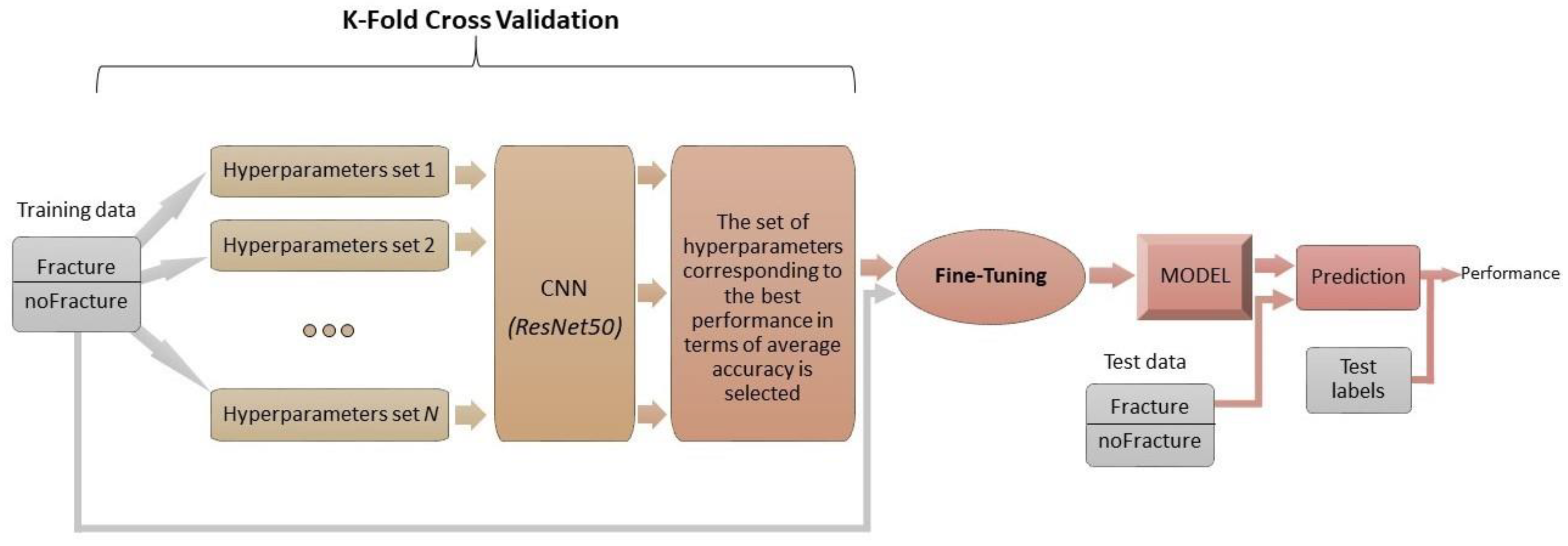
2.2. Experimental Setup Description
- K-fold cross validation to identify the hyperparameters (learning rate, weight decay, and drop out) that allow the network to have the highest performance in terms of accuracy;
- Fine-tuning of the network with the hyperparameters chosen in the previous step:
- 2.1
- Training only of the last layer;
- 2.2
- Unfreezing and training the whole model;
- Evaluation of the network’s performance.
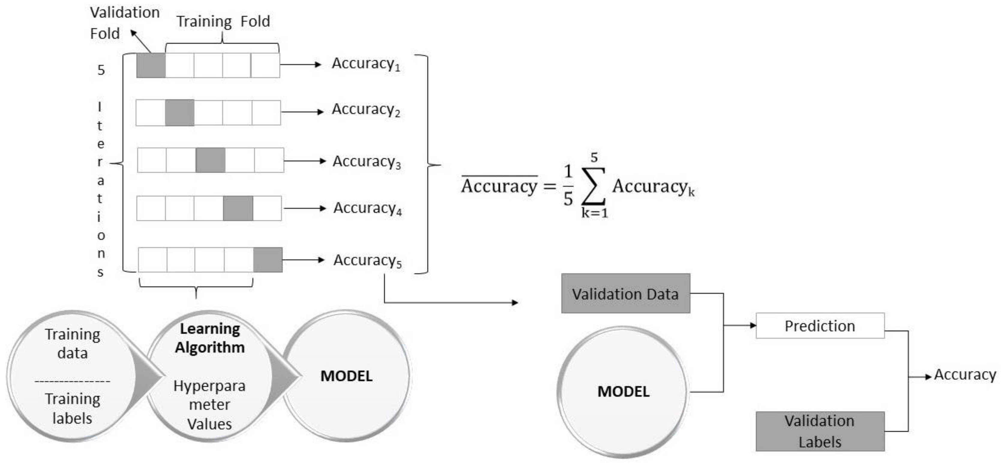
2.2.1. K-Fold Cross Validation
- Initial convolution (kernel size of 7 × 7) and max-pooling (kernel size of 3 × 3);
- Nine convolutional layers: kernel size of 1 × 1 and 64 different kernels, followed by kernel size of 3 × 3 and 64 different kernels, followed by kernel size of 1 × 1 and 256 different kernels. These three layers are repeated 3 times;
- Twelve convolutional layers: kernel size of 1 × 1 and 128 different kernels, followed by kernel size of 3 × 3 and 128 different kernels, followed by kernel size of 1 × 1 and 512 different kernels. These three layers are repeated 4 times;
- Eighteen convolutional layers: kernel size of 1 × 1 and 256 different kernels, followed by kernel size of 3 × 3 and 256 different kernels, followed by kernel size of 1 × 1 and 1024 different kernels. These three layers are repeated 6 times;
- Nine convolutional layers: kernel size of 1 × 1 and 512 different kernels, followed by kernel size of 3 × 3 and 512 different kernels, followed by kernel size of 1 × 1 and 2048 different kernels. These three layers are repeated 3 times;
- Average pooling layer followed by a fully connected layer with 1000 neurons and a softmax function at the end.
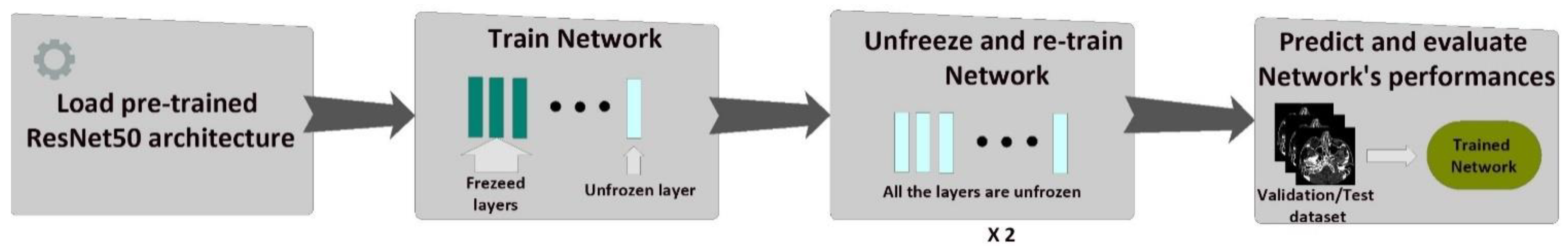
2.2.2. Fine-Tuning of the CNN
- Training of the last layer: we started with the pre-trained model’s weights (pre-trained on ImageNet), freezing all layers in the network’s body except the last layer. In this step, we trained only the last layer.
- Unfreezing and training the whole model: in this step, after the last layer had started to learn patterns of our medical dataset, we unfroze all the weights and trained the entire model with a very small learning rate. We wanted to avoid altering the convolutional filters dramatically.
3. Results
4. Discussion
4.1. Statement of Principal Findings
4.2. Strengths and Weaknesses of the Study
4.3. Strengths and Weaknesses in Relation to Other Studies, Discussing Particularly Any Differences in Results
4.4. Meaning of the Study: Possible Mechanisms and Implications for Clinicians or Policymakers
4.5. Unanswered Questions and Future Research
5. Conclusions
Author Contributions
Funding
Institutional Review Board Statement
Informed Consent Statement
Data Availability Statement
Acknowledgments
Conflicts of Interest
References
- Kalmet, P.H.S.; Sanduleanu, S.; Primakov, S.; Wu, G.; Jochems, A.; Refaee, T.; Ibrahim, A.; Hulst, L.V.; Lambin, P.; Poeze, M. Deep learning in fracture detection: A narrative review. Acta Orthop. 2020, 91, 215–220. [Google Scholar] [CrossRef] [Green Version]
- Esteva, A.; Kuprel, B.; Novoa, R.A.; Ko, J.; Swetter, S.M.; Blau, H.M.; Thrun, S. Dermatologist-level classification of skin cancer with deep neural networks. Nature 2017, 542, 115–118. [Google Scholar] [CrossRef]
- Gulshan, V.; Peng, L.; Coram, M.; Stumpe, M.C.; Wu, D.; Narayanaswamy, A.; Venugopalan, S.; Widner, K.; Madams, T.; Cuadros, J.; et al. Development and Validation of a Deep Learning Algorithm for Detection of Diabetic Retinopathy in Retinal Fundus Photographs. JAMA 2016, 316, 2402–2410. [Google Scholar] [CrossRef]
- Lee, J.-G.; Jun, S.; Cho, Y.-W.; Lee, H.; Kim, G.B.; Seo, J.B.; Kim, N. Deep Learning in Medical Imaging: General Overview. Korean J. Radiol. 2017, 18, 570–584. [Google Scholar] [CrossRef] [PubMed] [Green Version]
- Olczak, J.; Fahlberg, N.; Maki, A.; Razavian, A.S.; Jilert, A.; Stark, A.; Sköldenberg, O.; Gordon, M. Artificial intelligence for analyzing orthopedic trauma radiographs: Deep learning algorithms—are they on par with humans for diagnosing fractures? Acta Orthop. 2017, 88, 581–586. [Google Scholar] [CrossRef] [PubMed] [Green Version]
- Tang, A.; Tam, R.; Cadrin-Chênevert, A.; Guest, W.; Chong, J.; Barfett, J.; Chepelev, L.; Cairns, R.; Mitchell, J.R.; Cicero, M.D.; et al. Canadian Association of Radiologists White Paper on Artificial Intelligence in Radiology. Can. Assoc. Radiol. J. 2018, 69, 120–135. [Google Scholar] [CrossRef] [PubMed] [Green Version]
- Szegedy, C.; Liu, W.; Jia, Y.; Sermanet, P.; Reed, S.; Anguelov, D.; Erhan, D.; Vanhoucke, V.; Rabinovich, A. Going Deeper with Convolutions. In Proceedings of the IEEE Conference on Computer Vision and Pattern Recognition (CVPR), Boston, MA, USA, 7–12 June 2015; pp. 1–9. [Google Scholar]
- Kim, H.D.; MacKinnon, T. Artificial intelligence in fracture detection: Transfer learning from deep convolutional neu-ral networks. Clin. Radiol. 2018, 73, 439–445. [Google Scholar] [CrossRef] [PubMed]
- Szegedy, C.; Vanhoucke, V.; Ioffe, S.; Shlens, J.; Wojna, Z. Rethinking the Inception Architecture for Computer Vision. In Proceedings of the 2016 IEEE Conference on Computer Vision and Pattern Recognition (CVPR) 2016, Las Vegas, NV, USA, 27–30 June 2016. [Google Scholar]
- Chung, S.W.; Han, S.S.; Lee, J.W.; Oh, K.-S.; Kim, N.R.; Yoon, J.P.; Kim, J.Y.; Moon, S.H.; Kwon, J.; Lee, H.-J.; et al. Automated detection and classification of the proximal humerus fracture by using deep learning algorithm. Acta Orthop. 2018, 89, 468–473. [Google Scholar] [CrossRef] [Green Version]
- Tomita, N.; Cheung, Y.Y.; Hassanpour, S. Deep neural networks for automatic detection of osteopo-rotic vertebral fractures on CT scans. Comput. Biol. Med. 2018, 98, 8–15. [Google Scholar] [CrossRef]
- Heo, M.-S.; Kim, J.-E.; Hwang, J.-J.; Han, S.-S.; Kim, J.-S.; Yi, W.-J.; Park, I.-W. Artificial intelligence in oral and maxillofacial radiology: What is currently possible? Dentomaxillofacial Radiol. 2021, 50, 20200375. [Google Scholar] [CrossRef]
- Hung, K.; Montalvao, C.; Tanaka, R.; Kawai, T.; Bornstein, M.M. The use and performance of artificial intelligence applications in dental and maxillofacial radiology: A systematic review. Dentomaxillofacial Radiol. 2020, 49, 20190107. [Google Scholar] [CrossRef] [PubMed]
- Litjens, G.; Kooi, T.; Bejnordi, B.E.; Setio, A.A.A.; Ciompi, F.; Ghafoorian, M.; van der Laak, J.A.; van Ginneken, B.; Sánchez, C.I. A survey on deep learning in medical image analysis. Med. Image Anal. 2017, 42, 60–88. [Google Scholar] [CrossRef] [PubMed] [Green Version]
- Nagi, R.; Aravinda, K.; Rakesh, N.; Gupta, R.; Pal, A.; Mann, A.K. Clinical applications and performance of intelligent systems in dental and maxillofacial radiology: A review. Imaging Sci. Dent. 2020, 50, 81–92. [Google Scholar] [CrossRef]
- Python. Available online: https://www.python.org/ (accessed on 24 June 2021).
- PyTorch. Available online: https://pytorch.org/ (accessed on 3 July 2020).
- Fastai. Available online: https://docs.fast.ai/ (accessed on 3 February 2021).
- Scikit-Learn. Available online: https://scikit-learn.org/stable/ (accessed on 6 July 2020).
- Pydicom. Available online: https://pydicom.github.io/ (accessed on 8 July 2020).
- He, K.; Zhang, X.; Ren, S.; Sun, J. Deep residual learning for image recognition. In Proceedings of the IEEE Conference on Computer Vision and Pattern Recognition (CVPR), Las Vegas, NV, USA, 26 June–1 July 2016; pp. 770–778. [Google Scholar]
- Xie, S.; Girshick, R.; Dollar, P.; Tu, Z.; He, K. Aggregated Residual Transformations for Deep Neural Networks. In Proceedings of the 2017 IEEE Conference on Computer Vision and Pattern Recognition, Honolulu, HI, USA, 21–26 July 2017; pp. 1492–1500. [Google Scholar]
- Huang, G.; Liu, Z.; van der Maaten, L.; Weinberger, K.Q. Densely connected convolutional networks. In Proceedings of the IEEE Conference on Computer Vision and Pattern Recognition (CVPR), Honolulu, HI, USA, 22–25 July 2017; pp. 4700–4708. [Google Scholar]
- Russakovsky, O.; Deng, J.; Su, H.; Krause, J.; Satheesh, S.; Ma, S.; Huang, Z.; Karpathy, A.; Khosla, A.; Bernstein, M.; et al. ImageNet Large Scale Visual Recognition Challenge. Int. J. Comput. Vis. 2015, 115, 211–252. [Google Scholar] [CrossRef] [Green Version]
- Raschka, S. Model evaluation, model selection, and algorithm selection in machine learning. arXiv 2018, arXiv:1811.12808. [Google Scholar]
- Bergstra, J.; Bengio, Y. Random search for hyper-parameter optimization. J. Mach. Learn. Res. 2012, 13, 281–305. [Google Scholar]
- Learning Rate Finder. Available online: https://fastai1.fast.ai/callbacks.lr_finder.html (accessed on 3 February 2021).
- Howard, J.; Gugger, S. Fastai: A Layered API for Deep Learning. Information 2020, 11, 108. [Google Scholar] [CrossRef] [Green Version]
- Hanley, J.A.; McNeil, B.J. The meaning and use of the area under a receiver operating characteristic (ROC) curve. Radiology 1982, 143, 29–36. [Google Scholar] [CrossRef] [Green Version]
- Nicholls, A. Confidence limits, error bars and method comparison in molecular modeling. Part 1: The calculation of confidence intervals. J. Comput. Mol. Des. 2014, 28, 887–918. [Google Scholar] [CrossRef] [Green Version]
- Murero, M. Building Artificial Intelligence for Digital Health: A socio-tech-med approach and a few surveillance night-mares. Ethnogr. Qual. Res. Il Mulino 2020, 13, 374–388. [Google Scholar]
- Comelli, A.; Coronnello, C.; Dahiya, N.; Benfante, V.; Palmucci, S.; Basile, A.; Vancheri, C.; Russo, G.; Yezzi, A.; Stefano, A. Lung Segmentation on High-Resolution Computerized Tomography Images Using Deep Learning: A Preliminary Step for Radiomics Studies. J. Imaging 2020, 6, 125. [Google Scholar] [CrossRef]
- Gillies, R.J.; Kinahan, P.E.; Hricak, H. Radiomics: Images Are More than Pictures, They Are Data. Radiology 2016, 278, 563–577. [Google Scholar] [CrossRef] [Green Version]
- Pranata, Y.D.; Wang, K.-C.; Wang, J.-C.; Idram, I.; Lai, J.-Y.; Liu, J.-W.; Hsieh, I.-H. Deep learning and SURF for automated classification and detection of calcaneus fractures in CT images. Comput. Methods Programs Biomed. 2019, 171, 27–37. [Google Scholar] [CrossRef]


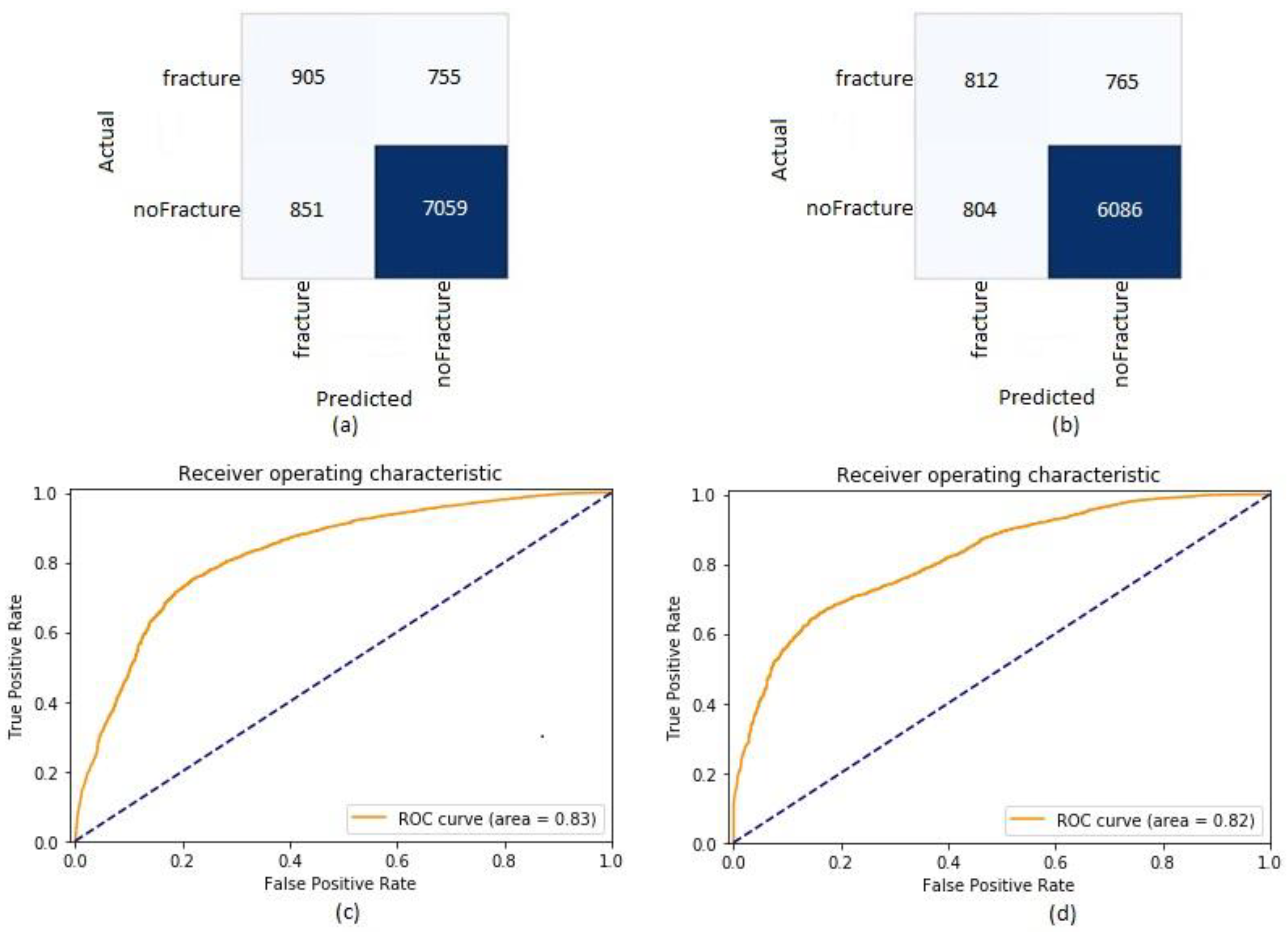
| Metric | Validation Dataset | Test Dataset |
|---|---|---|
| Accuracy | 0.83 (0.82, 0.84) | 0.81 (0.81, 0.82) |
| Recall | 0.55 (0.52, 0.57) | 0.51 (0.49, 0.54) |
| Precision | 0.52 (0.49, 0.54) | 0.50 (0.48, 0.53) |
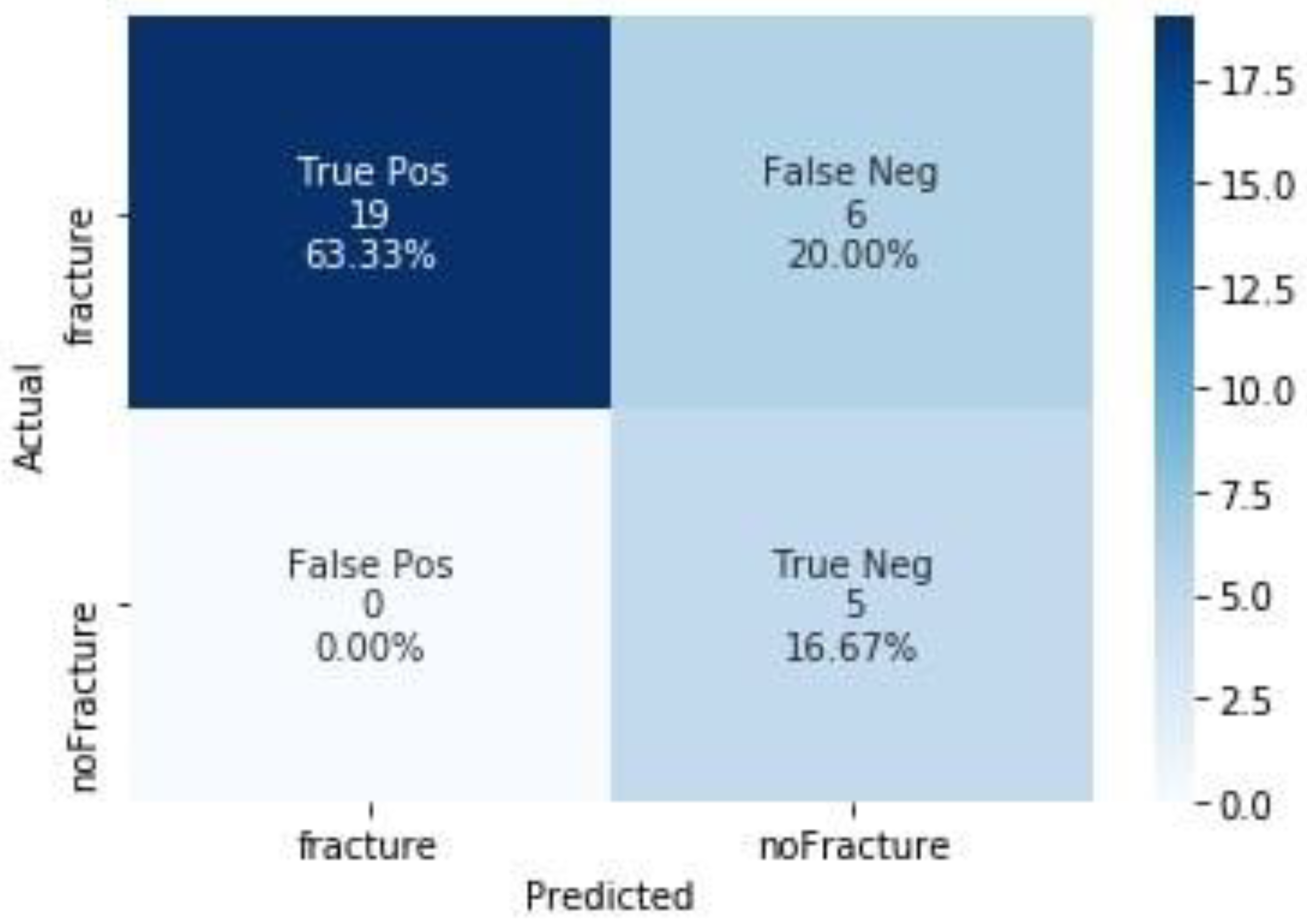
| Metric | Test Dataset |
|---|---|
| Accuracy | 0.80 (0.61, 0.92) |
| Recall | 0.76 (0.55, 0.91) |
| Precision | 1.0 (0.82, 1.00) |
Publisher’s Note: MDPI stays neutral with regard to jurisdictional claims in published maps and institutional affiliations. |
© 2021 by the authors. Licensee MDPI, Basel, Switzerland. This article is an open access article distributed under the terms and conditions of the Creative Commons Attribution (CC BY) license (https://creativecommons.org/licenses/by/4.0/).
Share and Cite
Amodeo, M.; Abbate, V.; Arpaia, P.; Cuocolo, R.; Dell’Aversana Orabona, G.; Murero, M.; Parvis, M.; Prevete, R.; Ugga, L. Transfer Learning for an Automated Detection System of Fractures in Patients with Maxillofacial Trauma. Appl. Sci. 2021, 11, 6293. https://doi.org/10.3390/app11146293
Amodeo M, Abbate V, Arpaia P, Cuocolo R, Dell’Aversana Orabona G, Murero M, Parvis M, Prevete R, Ugga L. Transfer Learning for an Automated Detection System of Fractures in Patients with Maxillofacial Trauma. Applied Sciences. 2021; 11(14):6293. https://doi.org/10.3390/app11146293
Chicago/Turabian StyleAmodeo, Maria, Vincenzo Abbate, Pasquale Arpaia, Renato Cuocolo, Giovanni Dell’Aversana Orabona, Monica Murero, Marco Parvis, Roberto Prevete, and Lorenzo Ugga. 2021. "Transfer Learning for an Automated Detection System of Fractures in Patients with Maxillofacial Trauma" Applied Sciences 11, no. 14: 6293. https://doi.org/10.3390/app11146293
APA StyleAmodeo, M., Abbate, V., Arpaia, P., Cuocolo, R., Dell’Aversana Orabona, G., Murero, M., Parvis, M., Prevete, R., & Ugga, L. (2021). Transfer Learning for an Automated Detection System of Fractures in Patients with Maxillofacial Trauma. Applied Sciences, 11(14), 6293. https://doi.org/10.3390/app11146293