Modified GSC Method to Reduce the Distortion of the Enhanced Speech Signal Using Cross-Correlation and Sidelobe Neutralization

Abstract

The generalized sidelobe canceller (GSC) method is a common algorithm to enhance audio signals using a microphone array. Distortion of the enhanced audio signal consists of two parts: the residual acoustic noise and the distortion of the desired audio signal, which means that the desired audio signal is damaged. This paper proposes a modified GSC method to reduce both kinds of distortion when the desired audio signal is a non-stationary speech signal. First, the cross-correlation coefficient between the canceling signal and the error signal of the least mean square (LMS) algorithm was added to the adaptive process of the GSC method to reduce the distortion of the enhanced signal while the energy of the desired signal frame was increased suddenly. The sidelobe pattern of beamforming was then presented to estimate the noise signal in the beamforming output signal of the GSC method. The noise component of the beamforming output signal was decreased by subtracting the estimated noise signal to improve the denoising performance of the GSC method. Finally, the GSC-SN-MCC method was proposed by merging the above two methods. The experiment was performed in an anechoic chamber to validate the proposed method in various SNR conditions. Furthermore, the simulated calculation with inaccurate noise directions was conducted based on the experiment data to inspect the robustness of the proposed method to the error of the estimated noise direction. The experiment data and calculation results indicated that the proposed method could reduce the distortion effectively under various SNR conditions and would not cause more distortion if the estimated noise direction is far from the actual noise direction.

1. Introduction

Online meetings are widely used in the current time. The quality of meeting audio has become increasingly important. Some problems of meeting audio, such as interfering speech, background noise, and speech reverberation, could be alleviated using several signal-processing methods with a single-channel microphone. These problems are all related to the spatial direction. Therefore, a multichannel microphone array is used to extract the desired signal by analyzing the spatial information of signals.

The primary method of a microphone array is the delay-and-sum beamforming (DSB) method presented by Flanagan et al. [1]. The multichannel signals are aligned at the look direction by compensation with the proper delay. The aligned signals are summed to ensure that the gain of the look direction is maximized. In other words, the signals from other directions are suppressed. More microphones should be employed to suppress the non-look direction signal more effectively. Capon [2] proposed the minimum variance distortionless response (MVDR) method in 1969 to achieve better denoising performance without increasing the number of microphones. The weight coefficients of different channels were adjusted to preserve the gain of the look direction and decrease the total power of the final output signal. Frost [3] developed the MVDR method that extended the constraint in the MVDR method to linear equations. Therefore, the weight coefficients could be adjusted adaptively based on the constraints. This method is referred to as the linearly constrained minimum variance (LCMV) method.

The constraints could be independent of the LCMV method to simplify the algorithm. Griffiths and Jim [4] proposed the generalized sidelobe canceller (GSC) method in 1982. The GSC method consisted of three parts. The first part is the same as a conventional beamforming method to reduce the noise roughly. The second part is a block matrix to generate a reference noise signal by removing the desired signal from the original multichannel signals. The third part is an adaptive filter to estimate the noise component of the first part’s output signal. Then, the estimated noise is subtracted from the output signal of the first part to obtain a cleaner desired signal. The GSC method converts the optimization goal of the LCMV method from the optimal weights with constraints to the optimal weights without constraints. Therefore, the simple adaptive algorithm could be adopted to reduce the residual noise in the final output signal.

The three parts of the GSC method could be optimized individually to improve the aggregate denoising performance of the adaptive algorithm. Hoshuyama et al. [5] and Lee et al. [6] modified the block matrix to decrease the sensitivity of the GSC method to a mismatch between the estimated and actual direction of arrival (DOA) of the desired signal. The robustness of the GSC method was increased by reducing the leakage of the desired signal into the reference noise signal [7]. Gannot et al. [8] considered the complicated acoustic environments and proposed a transfer function GSC (TF-GSC). The block matrix of the TF-GSC method was modified with the transfer function ratio (between different microphones in an array) to adapt the GSC method to reverberation conditions. Reuven et al. [9] combined the TF-GSC with an acoustic echo cancellation to improve the performance of the algorithm in noisy and reverberant environments. Reuven et al. [10] also extended the TF-GSC method to the DFT-GSC method for double talk scenarios to cancel the nonstationary interferences signal. Rombouts et al. [11] estimated a room impulse response and a desired speech signal model jointly to reduce the computational complexity dramatically for specific applications. Krueger et al. [12] estimated the acoustical transfer function ratios in the presence of stationary noise and tracked the eigenvector adaptively to obtain better noise and interference reduction. The GSC method also could be optimized by using efficient complex value arithmetic to reduce the calculation complexity [13] and by introducing the external microphones into the local microphone array to improve the performance of the speech estimate [14].

The least mean square (LMS) algorithm is a common adaptive algorithm for the GSC method to estimate the noise signal. The LMS algorithm adjusts the filter coefficients to make the mean square of the error signal (difference between the canceling signal and the received noise signal) lowest [15,16]. The stochastic gradient descent method has been used to ensure that the error signal can be decreased iteratively in real-time, which was derived by Widrow and Hoff [17] in 1960. Several modified LMS algorithms were proposed for some practical consideration. Nagumo and Noda [18] introduced the normalized LMS (NLMS) algorithm to make the algorithm convergence speed independent of the reference signal power, because the step size of the filter coefficient updating was inversely proportional to the reference signal power. Shan and Kailath [19] proposed the correlation LMS algorithm, which adjusted the step size of the filter coefficient updating to be proportional to the cross-correlation coefficient between the reference signal and the error signal. This means that when the reference signal and the error signal are uncorrelated, the step size will be too small to update the weight coefficients of the adaptive filter. This step size control scheme makes the adaptive algorithm more robust to disturbances, such as the system-measured noise. Gitlin et al. [20] proposed the leaky LMS algorithm, in which a leakage factor was added to the adaptive weight update path. The leakage factor could avoid the overflow of the unconstrained weight to increase the stability of the algorithm.

Some studies [21,22,23] introduced post-filtering methods to the microphone array for additional noise reduction to the beamforming output signal. Some studies [24,25,26] decomposed the multichannel signal into two subspace domains, the desired signal subspace domain and noise signal subspace domain, based on statistic features (like the singular value decomposition of the covariance matrix of the multichannel signal). The signal in the noise subspace domain was removed or suppressed, and the desired signal was restored from the desired signal subspace domain. Some researchers [27,28] attempted to extract the desired signal that had been contaminated by noise without a signal model or transmission model, which can be referred to as blind source separation or independent component analysis, most of which were based on the statistic features or a neural network. This research is mainly in the laboratory stage because of the complexity of calculation and the feasibility in actual environments.

The distortion of the enhanced signal consists of two parts: the residual noise and the distortion of the desired signal, which means that the desired signal is damaged. Most researchers attempted to reduce the residual noise of the output of the microphone array. In contrast, the desired signal is sometimes a nonstationary signal, as in speech application. The varying speech signal may damage the desired signal and degrade the denoising performance of the adaptive algorithm. Some researchers [29] employed the voice activity detection (VAD) method to make the algorithms only to be adjusted in speech-absent frames and avoid the affection of a varying speech signal. On the other hand, the VAD method is not always practical, especially when the background noise is heavy or the sound field is complex.

In this study, the conventional GSC method was modified to reduce the enhanced speech distortion without the VAD method. The step size of the adaptive algorithm in the GSC method was controlled by the cross-correlation coefficient between the cancelling signal and the error signal to reduce the distortion that occurred by the change of the speech energy. Furthermore, based on the excess mean-square error (MSE) of the LMS algorithm [30,31] and the theoretical limits of the noise reduction performance [32], the sidelobe neutralization (SN) method was presented to reduce the noise component in the beamforming output signal of the GSC method to improve the denoising performance.

This paper is organized as follows. Section 1 introduces the research background and reviews the relative academic achievements. Section 2 proposes the GSC method with the sidelobe neutralization method and the GSC method with the cross-correlation coefficient method. The modified GSC algorithm is given by combining them. Section 3 presents the implementation of the experiment and the result analysis. Section 4 provides the conclusions of this study.

2. The Proposed Method

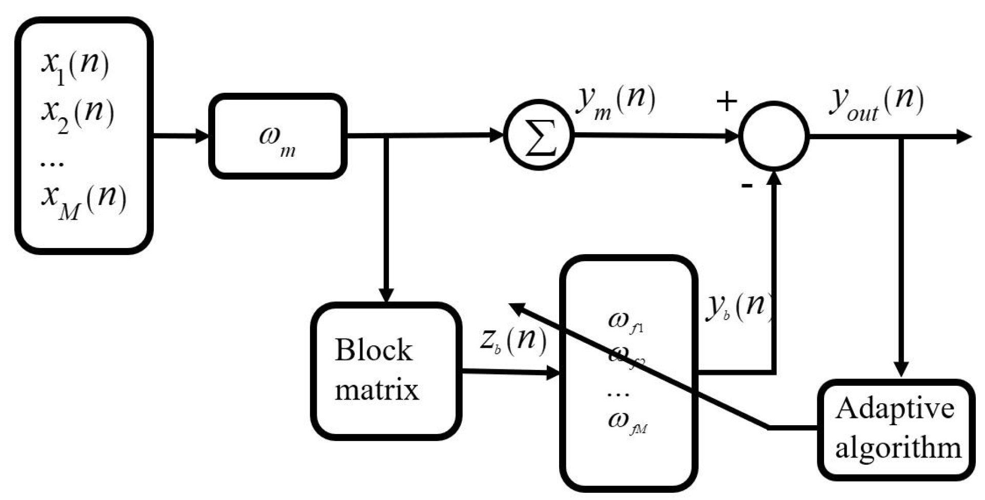
2.1. The Conventional GSC Method

The GSC algorithm can be separated into two transmission paths: the primary path and auxiliary path, as shown in Figure 1. The primary path generates a denoising signal with residual noise by the fixed beamforming method. The auxiliary path estimates the noise component in the output signal of the primary path. ω_m is the weight vector to make the microphone array signal x(n) aligned in the look direction to suppress noise from the other direction. y_m(n) is the sum of the aligned signals as the beamforming output signal of the primary path. The auxiliary path estimates the noise component y_b(n) in the beamforming output signal of the primary path as the cancelling signal. The cancelling signal will be removed from the beamforming output signal. Hence, the enhanced signal y_out(n) consists of the desired signal, and the residual noise signal is obtained.

The block matrix (BM) is adopted to generate the reference noise signal, excluding the desired signal from the noisy signal, in the auxiliary path for estimating the noise component of the beamforming output signal. Various methods can be used to design the block matrix for different purposes. The typical block matrix is as follows:

BM = [1 −1 0 0 … 0 0
0 1 −1 0 … 0 0
…
0 0 0 0 … 1 −1]_(M−1)*M

where M is the number of microphones in the microphone array. This matrix can block the desired signal completely in theory and introduce a low calculation complexity. The output z_b(n) of the block matrix is offered to the adaptive filter as the reference noise signal to estimate the noise component of the beamforming output signal. The LMS algorithm is commonly used as an adaptive filter to adjust the filter coefficients ω_f. Thus, the error signal of the LMS algorithm y_out(n), which is also the output signal of the GSC method, is obtained by removing the estimated noise signal from the beamforming output signal. The filter coefficient ω_f is then updated based on the reference noise signal and error signal.

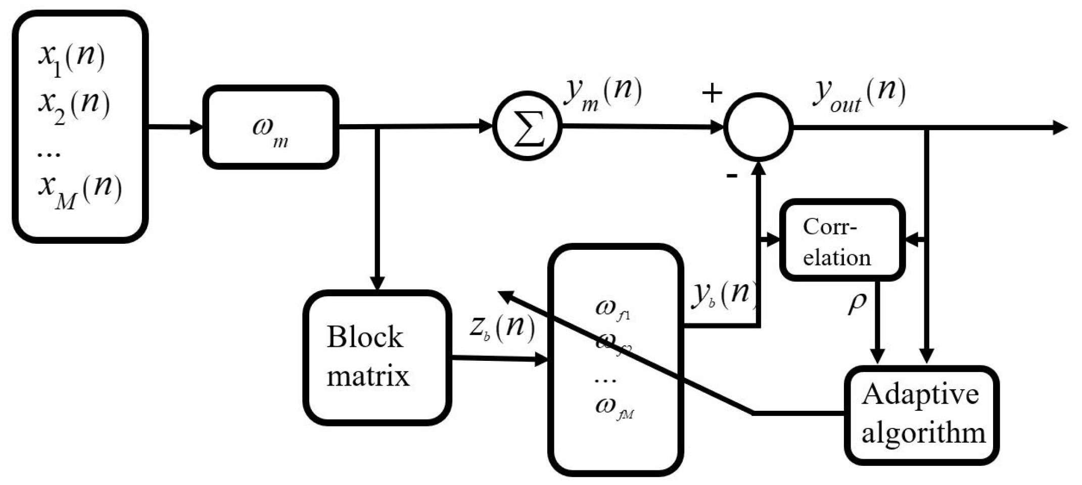
2.2. GSC Method with Cross-Correlation Coefficient

In practice, the error signal of the GSC method consists of a residual noise signal and an enhanced desired signal. In speech application, the desired signal is often a non-stationary speech signal. When the amplitude of the speech signal increases suddenly, the amplitude of the error signal should also be increased synchronously, while the amplitude of the residual noise signal may remain stable. Hence, over-subtraction may be caused in the subsequent frames. This problem can be solved using the GSC method with the cross-correlation coefficient (GSC-CC). In this method, the cross-correlation coefficient is introduced to the weight updating path, as shown in Figure 2. Because the speech signal usually is uncorrelated with noise signal in practical situations, the cross-correlation coefficient between the estimated noise y_b(n) and the error signal y_out(n) is used to control the step size of the adaptive filter weight update process, as expressed in the following equations.

$$w_f(n+1)=w_f(n)+\left|\rho (k-1)\right|\mu x(n)e(n)$$

(1)

$$\begin{array}{c}\rho \left(k\right)=E\left(y_b\left(k\right)y_{out}\left(k\right)\right)=E\left(y_b\left(k\right)\left(s_{speech}\left(k\right)+n_{residual}\left(k\right)\right)\right)\\ \hspace{1em}\hspace{1em}=E\left(y_b\left(k\right)s_{speech}\left(k\right)\right)+E\left(y_b\left(k\right)n_{residual}\left(k\right)\right)\end{array}$$

(2)

$$\mathrm{If}{y}_b\left(k\right)\approx n_{beamform}\left(k\right),\mathrm{thus}E\left(y_b\left(k\right)s_{speech}\left(k\right)\right)\approx 0,$$

(3)

$$\mathrm{Finally},\rho \left(k\right)\approx E\left(y_b\left(k\right)n_{residual}\left(k\right)\right),$$

(4)

where ρ(k) is the cross-correlation coefficient of the kth frame between the estimated noise y_b(k) and the error signal y_out(k). s_speech(k) represents the clean desired speech signal, and n_residual(k) is the residual noise component of the output signal. Because the speech signal is commonly assumed to be uncorrelated with the noise signal, the cross-correlation coefficient between the estimated noise and the speech signal is close to zero and can be neglected. Therefore, ρ(k) is equal to the cross-correlation coefficient between the estimated noise signal y_b(k) and the residual noise signal n_residual(k) as expressed in Equation (4). This means that if the ρ(k) is small, the residual noise is nearly uncorrelated with the estimated noise, so the weight coefficient will be changed only slightly. Otherwise, the weight coefficient will be changed considerably to reduce the residual noise rapidly.

Figure 3 and Figure 4 illustrate the influence of the varying speech signal on the estimated noise signal. The input original of a speech signal was extracted from the TIMIT database [33], and the noise signal was the white noise obtained from the NOISEX-92 database [34]. Figure 3a shows the original speech and noise signal, in which the signal-to-noise ratio (SNR) was equal to −5 dB (the ratio of the energy of the whole speech signal and the energy of the noise signal during the same time). Detailed information about the experiment implementation is depicted in Section 3. Figure 3b presents the cross-correlation coefficient between the estimated noise signal and the output signal with the conventional GSC method and the GSC-CC method. The negative peak of the cross-correlation coefficient with the conventional GSC method was generated when the amplitude of the speech signal increased suddenly (Figure 3b), which implies the phenomenon of over-subtraction.

Figure 4 compares the energy of the estimated noise frame with different methods. Figure 4b displays the partially enlarged view of Figure 4a from the 50th to the 100th frame. The energy of the estimated noise frame with the conventional GSC method would increase when the energy of the speech frame was much more than the actual noise frame. The GSC-CC method could flatten the energy curve of the estimated noise frame, which is consistent with the trend of the energy curve of the original white noise signal. This means that the distortion of the enhanced speech signal was reduced for the desired signal, and it was damaged less when the amplitude of the speech signal changed.

The GSC-CC method could decrease the overestimation of the noise efficiently when the desired speech signal amplitude was increased suddenly (Figure 4). On the other hand, the figures also show that the energy curve of the estimated noise frames with the GSC-CC method was lower than the conventional GSC method. As the correlation coefficient was less than or equal to one, the step size of the adaptive filter of the GSC-CC method was smaller than the GSC method. Consequently, the energy of the residual noise signal with the GSC-CC method was higher than the conventional GSC method.

The GSC method with the minimum cross-correlation coefficient (GSC-MCC) method was proposed by combining the conventional GSC method and the GSC-CC method to utilize the advantages of the two methods. The conventional GSC method and the GSC-CC method ran synchronously. The output signal frame, which had the smaller cross-correlation coefficient (between the estimated noise signal and the corresponding output signal) of the two methods, was adopted to synthesize the final output signal. Considering the overlap of speech frames and the nonstationary nature of a speech signal, the principle of the GSC-MCC method to choose the frame to synthesize the final output signal was modified using Equation (5).

$$y_{out-final}(k)=\{\begin{array}{l}{y}_{out-corr}(k),\hspace{1em}\hspace{1em}{\displaystyle \sum _{i=k-1}^{k+1}sign\left(\left|{\rho }_{con\nu }\left(i\right)\right|-\left|{\rho }_{corr}\left(i\right)\right|\right)\ge 2}\\ y_{out-con\nu }(k),\hspace{1em}\hspace{1em}otherwise\end{array},$$

(5)

where y_out-corr(k) and y_out-conv(k) represent the output signal frame of the GSC-CC method and the conventional GSC-CC method, respectively.

2.3. GSC Method with Sidelobe Neutralization

2.3.1. Beamforming Pattern

In this study, the microphone array was assumed to be a uniform circle array (UCA), with M microphones deployed uniformly on a circle with a radius of r. The sound source and the microphone array were assumed to be on the same horizontal plane for convenience. That is, the incident elevation angle of the desired signal and the noise signal both were 0°. The sound source direction vector ν was obtained as shown Equation (8), based on the angle interval α_m and relative distance x_r between microphones.

$${\alpha }_m=2\pi (m-1)/M$$

(6)

$$x_r=r·\cos \left(\varphi -{\alpha }_m\right)$$

(7)

$$\nu ={\left[e^{j(k{x}_{r1})},e^{j(k{x}_{r2})},\dots ,e^{j(k{x}_{rM})}\right]}^T$$

(8)

Thus, the beamforming pattern could be derived using the following equations [35]:

$$B\left({\varphi }_s,{\varphi }_i\right)={\displaystyle \sum _{m=1}^M{\omega }_{(s,m)}^{\ast }{\nu }_{(i,m)}}=\frac{1}{M}{\displaystyle \sum _{m=1}^M{e}^{j2kr\sin (\frac{{\varphi }_s-{\varphi }_i}{2})\sin (\frac{{\varphi }_s+{\varphi }_i}{2}-{\alpha }_m)}}=\frac{1}{M}{\displaystyle \sum _{m=1}^M\exp \left(-jz\sin \left(\beta -{\alpha }_m\right)\right)},$$

(9)

where

$$z=2kr\sin (\frac{{\varphi }_s-{\varphi }_i}{2}),\beta =\frac{{\varphi }_s+{\varphi }_i}{2},$$

(10)

and ω_(s,m) is the weight of the microphone channel to adjust the look direction Φ_s of the microphone array. Φ_i represents the actual incident direction of the sound source.

Based the Jacobi–Anger identity,

$$\exp \left(jz\sin \left(\alpha \right)\right)={\displaystyle \sum _{n=-\infty }^{\infty }{J}_n\left(z\right)\exp \left(jn\alpha \right)}$$

(11)

where J_n is the nth-order Bessel function; let b = n/M,

$$\mathrm{Final}:B\left({\varphi }_s,{\varphi }_i\right)={\displaystyle \sum _{b=-\infty }^{\infty }{J}_{bM}\left(z\right)\exp \left(-jbM\beta \right)},$$

(12)

$$\mathrm{If}M\mathrm{is}\mathrm{even}:B\left({\varphi }_s,{\varphi }_i\right)=J_0\left(z\right)+2{\displaystyle \sum _{b=1}^{\infty }{J}_{bM}\left(z\right)\cos \left(bM\beta \right)},$$

(13)

Consequently, the beamforming pattern could be formed by the Bessel functions. Considering the property of the Bessel function, the value of the second item of Equation (13) will be close to zero and can be neglected with an increasing number of microphones. Thus, the beamforming pattern could be approximated as a zero-order Bessel function.

2.3.2. Beamforming Sidelobe Neutralization

When the configuration of the microphone array was determined, the sidelobe of the beamforming pattern could be calculated as in Equation (13). If there are two sound sources, s₁ and s₂, deployed in the direction vector ν₁ and ν₂, respectively, in the sound field, the sidelobe neutralization method could be derived using the following equations:

$$S=\left[s_1,s_2\right],\nu =\left[{\nu }_1,{\nu }_2\right];$$

(14)

the received signal of microphones x_m could be written as:

$$x_m=S\nu =s_1{\nu }_{(1,m)}+s_2{\nu }_{(2,m)}$$

(15)

The output signal of the beamforming function to the corresponding direction is:

$$y_{\nu 1}={\displaystyle \sum _{m=1}^M{\omega }_{(s1,m)}^{\ast }{x}_m}={\displaystyle \sum _{m=1}^M{\nu }_{(1,m)}^{\ast }{s}_1{\nu }_{(1,m)}+{\nu }_{(1,m)}^{\ast }{s}_2{\nu }_{(2,m)}}=s_1+{\displaystyle \sum _{m=1}^M{\nu }_{(1,m)}^{\ast }{s}_2{\nu }_{(2,m)}}$$

(16)

$$y_{\nu 2}={\displaystyle \sum _{m=1}^M{\omega }_{(s2,m)}^{\ast }{x}_m}={\displaystyle \sum _{m=1}^M{\nu }_{(2,m)}^{\ast }{s}_1{\nu }_{(1,m)}+{\nu }_{(2,m)}^{\ast }{s}_2{\nu }_{(2,m)}}=s_2+{\displaystyle \sum _{m=1}^M{\nu }_{(2,m)}^{\ast }{s}_1{\nu }_{(1,m)}}$$

(17)

$$\mathrm{Let}{u}_{ab}={\displaystyle \sum _{m=1}^M{\nu }_{(a,m)}^{\ast }{\nu }_{(b,m)}}=B\left({\varphi }_a,{\varphi }_b\right),$$

(18)

$$y_{\nu 1s2}=y_{\nu 1}-u_{12}{y}_{\nu 2}=s_1+u_{12}{s}_2-u_{12}{s}_2-u_{12}{u}_{21}{s}_1=s_1\left(1-u_{12}{u}_{21}\right)=s_1\left(1-{\left|u_{12}\right|}^2\right)$$

(19)

where u_ab represents the attenuation coefficient of the sidelobe when the sound source is placed at direction b and beamformed to direction a. Moreover, the attenuation coefficient will be the conjugate of u_ab when the cast direction is inverse.

Hence, Equation (19) could be used for direction ν₁ to reduce the noise received from direction ν₂. This equation proves that the noise signal from the interference direction can theoretically be removed entirely from the beamforming output signal of the look direction. When the attenuation coefficient is not equal to one, the signal amplitude from the look direction could be maintained by multiplying a proper scale factor. On the other hand, if the attenuation coefficient of the frequency is equal to one, this frequency signal would be lost completely and could not be compensated.

Therefore, the sidelobe neutralization method could be modified as in Equations (20) and (21). The desired signal component in the noise direction was calculated and subtracted from the beamforming output of the noise direction as in Equation (20). Hence, the estimated noise signal becomes the pure noise without the desired signal. The output of the sidelobe neutralization method was calculated using Equation (21). This equation proves that the sidelobe neutralization method would not miss the frequency signal with an attenuation coefficient of even one. Because most of the time, u_ab is less than 1, the cube of u_ab is less than itself. Combining Equations (16) and (21), it means that (u₁₂)³ should be less than u₁₂ most of the time. Thus, the beamforming output with less noise is obtained.

$$y_{\nu 2s1}=y_{\nu 2}-u_{21}{y}_{\nu 1}=s_2+u_{21}{s}_1-u_{21}{s}_1-u_{21}{u}_{12}{s}_2=s_2\left(1-u_{21}{u}_{12}\right)=s_2\left(1-{\left|u_{21}\right|}^2\right)$$

(20)

$$y_{\nu 1s2s1}=y_{\nu 1}-u_{12}{y}_{\nu 2s1}=s_1+u_{12}{s}_2-u_{12}{s}_2\left(1-{\left|u_{21}\right|}^2\right)=s_1+s_2{\left(u_{12}\right)}^3$$

(21)

However, the estimated noise direction is often inaccurate in practice. The error of the estimated noise direction would affect the performance of the sidelobe neutralization method. ν₃ is assumed to be the inaccurately estimated noise direction, and Equations (20) and (21) can be modified as follows:

$$y_{\nu 3}={\displaystyle \sum _{m=1}^M{\omega }_{(s3,m)}^{\ast }{x}_m}={\displaystyle \sum _{m=1}^M{\nu }_{(3,m)}^{\ast }{s}_1{\nu }_{(1,m)}+{\nu }_{(3,m)}^{\ast }{s}_2{\nu }_{(2,m)}}=u_{31}{s}_1+u_{32}{s}_2$$

(22)

$$y_{\nu 3s1}=y_{\nu 3}-u_{31}{y}_{\nu 1}=u_{31}{s}_1+u_{32}{s}_2-u_{31}{s}_1-u_{31}{u}_{12}{s}_2=s_2\left(u_{32}-u_{31}{u}_{12}\right)$$

(23)

$$y_{\nu 1s3s1}=y_{\nu 1}-u_{13}{y}_{\nu 3s1}=s_1+u_{12}{s}_2-u_{13}{s}_2\left(u_{32}-u_{31}{u}_{12}\right)=s_1+s_2\left[u_{12}-u_{13}\left(u_{32}-u_{31}{u}_{12}\right)\right]$$

(24)

$$\mathrm{Let}{r}_{\nu 3}=\left|\frac{u_{12}-u_{13}\left(u_{32}-u_{31}{u}_{12}\right)}{u_{12}}\right|,$$

(25)

where r_ν3 is the ratio of the noise signal processed by the sidelobe neutralization method with the inaccurate noise direction to that by the beamforming method. r_ν3 can be analyzed qualitatively as follows:

If u₁₂ is small or near to zero, thus,

$$y_{\nu 1s3s1}=s_1+s_2\left[u_{12}-u_{13}\left(u_{32}-u_{31}{u}_{12}\right)\right]=s_1+s_2\left(-u_{13}{u}_{32}\right)$$

(26)

Therefore, r_ν3 may be extremely big.

If u₁₂ is big, there are roughly two cases:

$$(1){\nu }_3\mathrm{is}\mathrm{near}{\nu }_2;\mathrm{thus},r_{\nu 3}=\left|1-\frac{u_{13}{u}_{32}}{u_{12}}+u_{13}^2\right|\approx \left|1-\frac{u_{12}{u}_{22}}{u_{12}}+u_{13}^2\right|=u_{13}^2\le 1,$$

(27)

$$(2){\nu }_3\mathrm{is}\mathrm{far}\mathrm{from}{\nu }_2;\mathrm{thus},u_{32}\mathrm{is}\mathrm{small},r_{\nu 3}=\left|1-\frac{u_{13}{u}_{32}}{u_{12}}+u_{13}^2\right|\le \left|1+u_{13}^2\right|+\left|\frac{u_{32}}{u_{12}}\right|\le 3$$

(28)

Assume an instance, in which ν₁ is 0° and ν₂ is 60°, to illustrate the affection of the inaccurately estimated noise direction for the residual noise. According to Equation (25), Figure 5 shows r_ν3 with different estimated noise direction (ν₃ from −180° to +180°).

The blue gap near 60° in Figure 5a shows that the noise signal processed by the sidelobe neutralization method with an inaccurate noise direction was less than that by the original beamforming method in a relatively wide direction range near the actual noise direction. The ratio in the frequency band between 1000 to 1500 Hz in all directions was high, because the sidelobe attenuation coefficient of the actual noise direction in this frequency range was close to zero (u₁₂, as shown in Figure 5b).

When the estimated noise direction was far away from the actual noise direction, the ratio was close to one at the greatest portion of the figure, which means that the energy of the noise signal processed by the sidelobe neutralization method was almost equal to that by the beamforming method, except in the high-frequency band in several directions. Even in these areas, the ratio was still less than two.

Therefore, the conclusion could be derived that the sidelobe neutralization method could work effectively when the estimated noise direction was near the actual noise direction. When the estimated noise direction was far away from the actual noise direction, the denoising performance of the sidelobe neutralization method was similar to the beamforming method, except in the frequency range, in which the sidelobe attenuation of the actual noise direction was strong.

2.3.3. The GSC Method with Sidelobe Neutralization

In LMS theory, the denoising performance of the algorithm is relative to the energy of the received noise signal [30]. Therefore, the GSC-SN method was proposed by adding the sidelobe neutralization method to the primary path of the conventional GSC method. The sidelobe neutralization method was used to reduce the received noise to improve the performance of the GSC method. When the noise weight vector was estimated to be ω_n, the noise signal y_n(n) in the noise direction could be estimated using Equation (17). The desired signal in the noise direction y_nm(n) was calculated and subtracted from the estimated noise signal as in Equation (20). Therefore, the pure estimated noise signal y_nsm(n) was obtained without the desired signal. The pure estimated noise signal was subtracted from the beamforming output signal of the desired signal direction y_m(n). Thus, the beamforming output of the primary path with less noise was obtained as Equation (21). The denoising performance of the GSC method could be improved by the beamforming output signal with less noise.

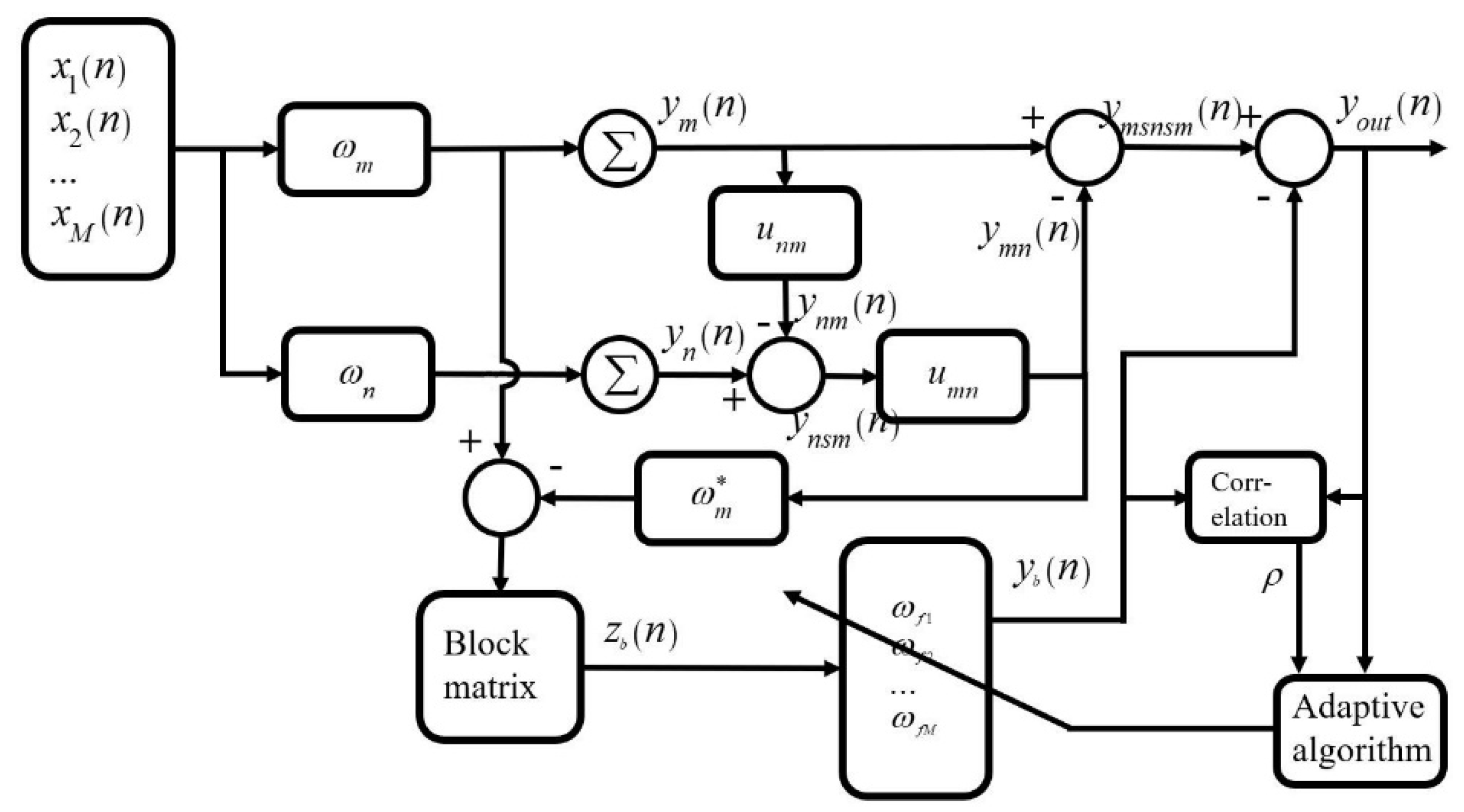
2.4. The Proposed GSC-SN-MCC Method

Finally, the GSC-SN-MCC method was proposed by combining the GSC-MCC method and the GSC-SN method to improve the performance of the GSC method. The GSC-MCC method was used to reduce the distortion of the enhanced signal caused by the varying desired signal. The sidelobe neutralization method was placed in the primary path of the GSC-MCC method to generate the beamforming output signal with less noise to improve the denoising ability of the proposed method.

As shown in Figure 6, the received signal of the microphone array was beamformed in the desired signal direction ω_m and the noise signal direction ω_n, respectively. Based on Equations (16), (17), (20) and (21), the beamforming output signal with less noise than the original beamforming method was obtained. Then, the system was run as the usual GSC method until updating the adaptive filter coefficient. The cross-correlation coefficient ρ (between the estimated noise signal and the corresponding output signal) was added to the adaptive filter coefficient updated equation to control the overestimating of the noise component, as in Equation (1).

3. Experiment and Analysis

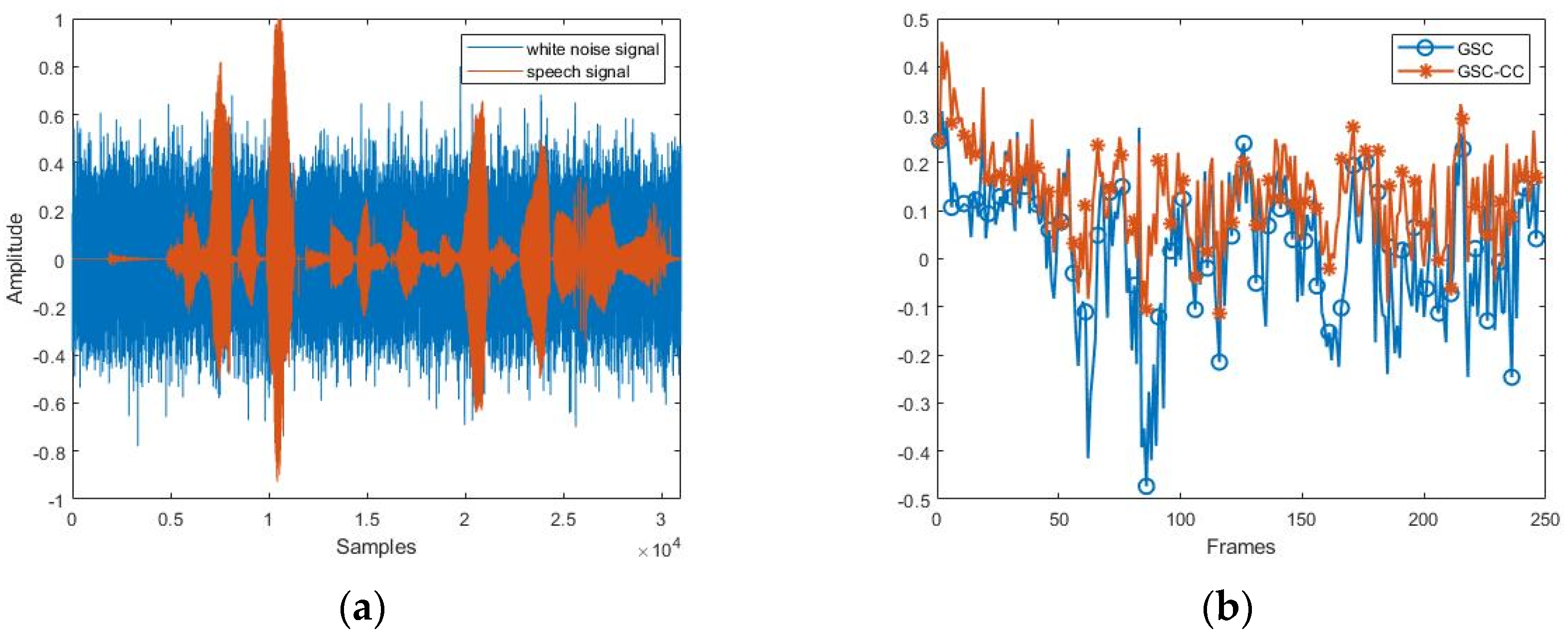
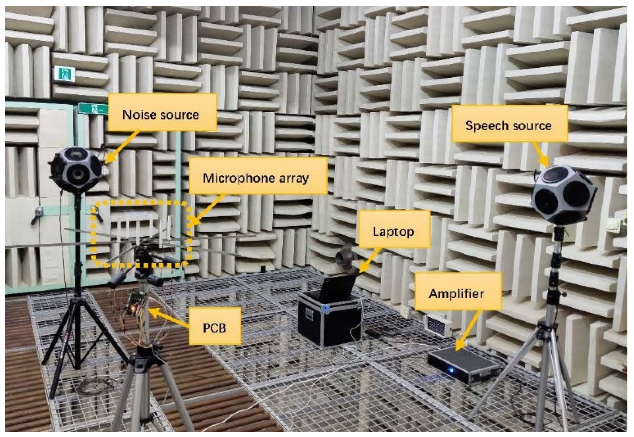
3.1. Experiment Implementation

The laboratory experiments were conducted in the anechoic chamber to validate the proposed method. The experimental layout is shown in Figure 7. The laptop was the control center to manage the audio system for simulating a real environment. Two omnidirectional speakers were connected to the laptop as the speech and noise sources, respectively, using an INTERM L-2400 power amplifier. The microphone array consisted of 6 MEMS microphones, distributed uniformly in a circle with a radius of 0.1 m. The printed circuit board (PCB) of the SCIEN company was connected to the microphones to realize the signal amplification function, the A/D conversion function, and transfer the digital signal to the laptop for recording. The signal was processed by the MATLAB software. To simplify the experiment, the speakers and the microphone array were deployed in the same horizontal plane. This means that the elevation angles of the incident signals (desired signal and noise signal) were 90°.

Based on the common far-field equation, expressed as in Equation (29), the minimum distance between the microphone array and the sound source was calculated to ensure that the position of the speakers satisfied the far-field condition. Assuming that the sound speed c is 343 m/s, the maximum frequency f was 4000 Hz, and the diameter of microphone array L was 0.2 m. Hence, the minimum distance d was approximately 0.933 m. Thus, the speakers were deployed about 2.5 m away from the microphone array, considering the space of the anechoic chamber and the minimum distance d. The azimuth angles of the speech signal source and the noise signal source were 0° and 90°, respectively.

$$d=2\ast L^2/\lambda =2\ast L^2\ast f/c$$

(29)

The speech of a female was selected randomly from the TIMIT database [32] as the desired signal. White noise in the NOISE-92 database [33] was chosen as the noise signal. The power of the noise signal was adjusted to simulate different SNR conditions. The sampling rate of the microphone array was 16,000 Hz, and the received signal was filtered using a lowpass filter, of which the cutoff frequency was 4000 Hz. The high sampling rate could increase the time resolution of the system and exhibit the phase difference between microphones more obviously. Because most of the energy of speech is concentrated in the low and medium frequency bands, the received signal was filtered by a lowpass filter to reduce the calculation burden of the hardware, while most of the speech information was preserved.

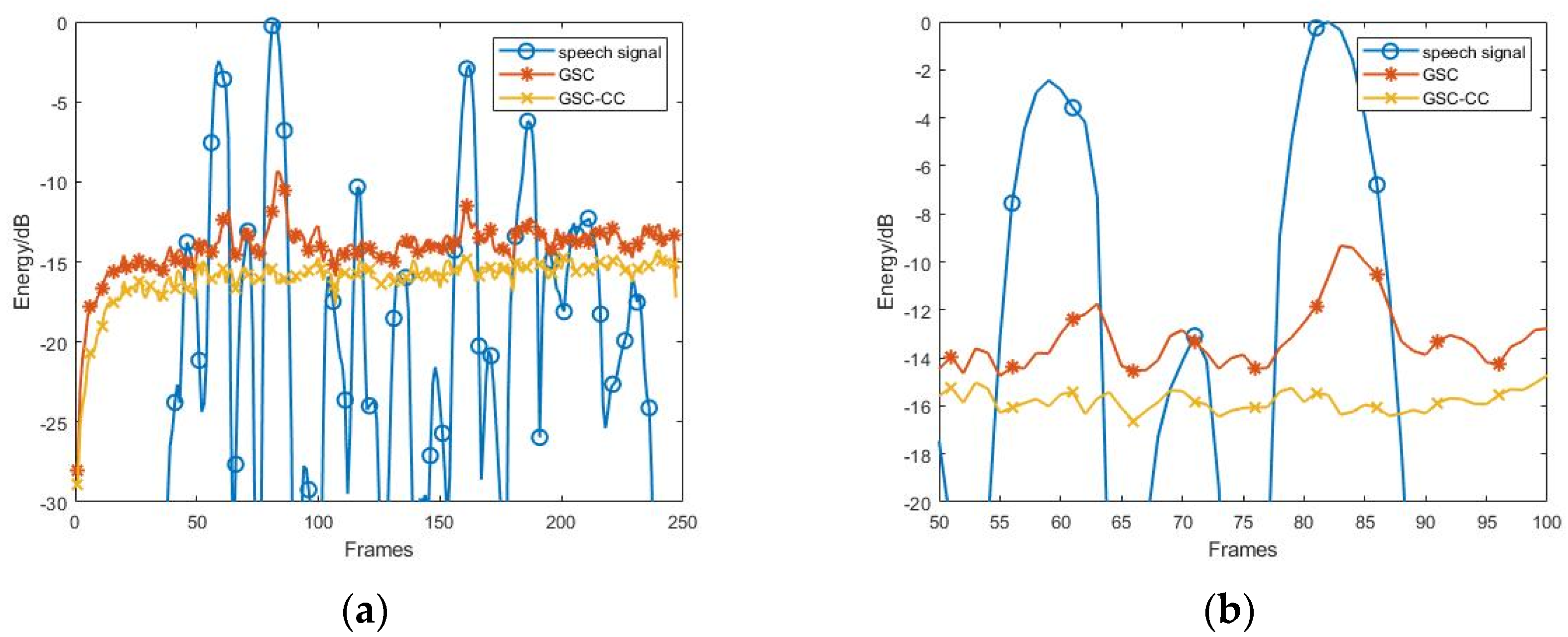
3.2. Experiment Result Analysis

3.2.1. Effect of the Various SNR Conditions

Figure 8 compares the distortion–noise ratio of frames with different methods while SNR is −5 dB. The distortion of the enhanced speech signal was calculated using Equation (30), where k represents the kth frame and l is the length of the frame. y_out(n) and s_speech(n) represent the output signal of the method and the clean desired speech signal without noise, respectively. Less distortion means better denoising performance of the method. Equation (31) calculates the distortion–noise ratio as the distortion divided by the pure noise energy.

$$distortion\left(k\right)={\displaystyle \sum _{n=k\ast l}^{(k+1)\ast l}{\left[y_{out}\left(n\right)-s_{speech}\left(n\right)\right]}^2}$$

(30)

$$p\left(k\right)=\left|\frac{distortion\left(k\right)}{noise\left(k\right)}\right|={\displaystyle \sum _{n=k\ast l}^{(k+1)\ast l}\frac{{\left[y_{out}\left(n\right)-s_{speech}\left(n\right)\right]}^2}{{\left[s_{noise}\left(n\right)\right]}^2}}$$

(31)

Figure 8b presents an enlarged view of Figure 8a from the 50th to 100th frames, which included two peaks of the speech frame energy. The figure shows that peaks of the signal distortion were generated using the GSC method when the energy of the speech frame was increased suddenly. The GSC-CC method could alleviate this problem, while the residual noise would increase at other frames where the speech energy is stable. The GSC-SN method could reduce the distortion of most frames caused by the residual noise, but the above-mentioned distortion problem with damage to the desired signal exists. The GSC-SN-MCC method could take advantage of the above methods to decrease both kinds of distortion of the enhanced signal.

The maximum distortion occurred at the 83^rd frame in this case, as shown in Figure 8. Figure 9 presents the spectrum of signal distortion of the 83rd frame where the fast Fourier transform was utilized. For convenience, the amplitude of the spectrum was normalized. Figure 9a shows the spectrum of signal distortion of the 83rd frame over the entire frequency band with different methods. When a different method was employed, there were apparent differences in the amplitude from 500 Hz to 2000 Hz, where the speech energy was concentrated. Figure 9b shows the enlarged view of this frequency band. The distortion spectrum with the GSC-SN-MCC method was smaller and flatter than the conventional GSC method. Hence, the distortion of the enhanced signal caused by damaging the desired signal was reduced successfully using the proposed method.

Table 1. Average of the distortion–noise ratio with different methods under various SNR conditions.

SNR/dB	GSC	GSC-CC	GSC-SN	GSC-SN-MCC
20	100%	65.98%	104.03%	75.75%
10	100%	57.93%	100.99%	46.29%
5	100%	54.46%	97.92%	38.51%
0	100%	72.66%	89.87%	44.14%
−5	100%	105.34%	83.98%	59.01%
−10	100%	134.85%	80.22%	72.41%
−20	100%	157.90%	77.21%	78.84%

Normalized to result of the GSC method.

and

Table 2. Distortion of the 83rd frame with different methods under various SNR conditions.

SNR/dB	GSC	GSC-CC	GSC-SN	GSC-SN-MCC
20	100%	54.09%	109.34%	82.73%
10	100%	39.69%	110.58%	40.31%
5	100%	20.91%	106.16%	20.94%
0	100%	17.68%	96.88%	17.11%
−5	100%	22.38%	93.10%	18.44%
−10	100%	38.14%	90.32%	27.24%
−20	100%	124.24%	80.42%	72.87%

Normalized to result of the GSC method.

list the denoising performance of different methods under various SNR conditions. Table 1 lists the average of the distortion–noise ratio, and Table 2 presents the distortion value of the 83rd frame (maximum distortion frame) under various conditions. For comparison, the average value of the distortion–noise ratio and the distortion value of the 83rd frame was normalized to the result of the GSC method, which was one, as shown in Equations (32) and (33). Table 2 indicates that the GSC-CC method could reduce the peak value of the enhanced signal distortion effectively under most SNR conditions, except that the noise was too heavy that the speech energy barely affected the estimation of the residual noise. The GSC-SN method showed better performance under low SNR conditions (Table 1). The proposed GSC-SN-MCC method was a combination of the above two methods. The tables show that the proposed method could work effectively under both high and low SNR conditions. The best performance of the proposed method occurred when the energy of speech was almost equal to the energy of noise.

$$r_p=\frac{a\nu g\left({\displaystyle \sum p_{method}\left(k\right)}\right)}{a\nu g\left({\displaystyle \sum p_{GSC}\left(k\right)}\right)}$$

(32)

$$r_d\left(k\right)=\frac{distortio{n}_{method}\left(k\right)}{distortio{n}_{GSC}\left(k\right)}$$

(33)

3.2.2. Effect of the Inaccurate Estimated Noise Direction

The simulation calculation was conducted based on the previous experiment data to show the influence on the performance of the proposed method when the estimated noise direction was not accurate. Therefore, the incident direction of the desired signal was 0°, and the actual noise direction was 90° in this section. The SNR condition was performed at −5 dB. Twelve angles were chosen as the inaccurately estimated noise directions, which were distributed uniformly in a circle. The meaning of the coordinate axes in the figures and the calculation equations of the result were the same as in the previous subsection.

Figure 10 presents the distortion–noise ratio of the frames with different methods when the estimated noise direction was 60°. Figure 10b is the enlarged view of Figure 10a from the 50th to 100th frame. Figure 11 shows the spectrum of signal distortion of the 83rd frame on the entire frequency band using different methods. Figure 11b displays the enlarged view of Figure 11a from 500 Hz to 2000 Hz.

The figures indicate that even with an error angle between the actual noise direction and the estimated noise direction of 30°, the proposed method could effectively reduce both the peak value and the average value of the signal distortion in this case.

Table 3. Average of the distortion–noise ratio with different methods in various estimated noise directions.

Estimated Noise Direction/Degree	GSC	GSC-CC	GSC-SN	GSC-SN-MCC
−60	100%	105.34%	112.55%	100.87%
−30	100%	105.34%	106.33%	91.93%
0	100%	105.34%	100%	88.07%
30	100%	105.34%	92.92%	76.27%
60	100%	105.34%	92.80%	68.32%
90	100%	105.34%	83.98%	59.01%
120	100%	105.34%	95.71%	80.68%
150	100%	105.34%	90.56%	76.15%
180	100%	105.34%	97.76%	82.98%
−150	100%	105.34%	94.29%	79.13%
−120	100%	105.34%	105.59%	93.54%
−90	100%	105.34%	102.98%	88.94%

Normalized to result of the GSC method.

and

Table 4. Distortion of the 83rd frame with different methods in various estimated noise directions.

Estimated Noise Direction/Degree	GSC	GSC-CC	GSC-SN	GSC-SN-MCC
−60	100%	22.38%	105.90%	24.68%
−30	100%	22.38%	97.81%	23.04%
0	100%	22.38%	100%	22.38%
30	100%	22.38%	94.42%	21.15%
60	100%	22.38%	103.73%	20.55%
90	100%	22.38%	93.10%	18.44%
120	100%	22.38%	103.00%	23.60%
150	100%	22.38%	89.81%	21.52%
180	100%	22.38%	98.23%	23.62%
−150	100%	22.38%	93.95%	22.44%
−120	100%	22.38%	102.58%	25.06%
−90	100%	22.38%	96.50%	23.57%

Normalized to result of the GSC method.

compare the performance of the different methods in various estimated noise directions. Table 3 shows that the performance of the GSC-SN method would decrease with the estimated noise direction far away from the actual noise direction. The GSC-SN method would reduce to the conventional GSC method when the estimated noise direction was identical to the desired signal direction. When the estimated noise direction was identical to the actual noise signal direction, the GSC-SN method would achieve the best denoising performance. The trend of the performance of the proposed GSC-SN-MCC method was similar to the GSC-SN method. Better performance of the proposed method could be attained if the estimated noise direction was closer to the actual noise direction. Even when the estimated noise direction was the opposite of the actual noise direction, the performance of the proposed method was still not worse than the conventional GSC method. Table 4 lists the GSC-CC method that could reduce the peak value of the signal distortion, which was independent of the estimated noise direction. The ability to decrease the peak of the enhanced signal distortion by the proposed method was similar to the GSC-CC method.

The tables show that the proposed method could work effectively when the estimated noise direction was near the actual noise direction. When the estimated noise direction was far from the actual noise direction, the proposed method could still reduce the peak value of the enhanced signal distortion effectively, and the average of the enhanced signal distortion using the proposed method was similar to the conventional GSC method.

4. Conclusions

This paper proposed a modified GSC method to reduce the distortion of the enhanced signal using cross-correlation and sidelobe neutralization. The GSC-MCC method was proposed first by adding the cross-correlation coefficient between the cancelling signal and the error signal to the filter weight update path to control the distortion of the enhanced desired signal when the energy of the desired signal was increased suddenly. The beamforming sidelobe pattern was presented and combined with the conventional GSC method (refer to the GSC-SN method) to improve the denoising performance of the GSC method by reducing the noise component in the beamforming output signal of the GSC method. Finally, the GSC-SN-MCC method was proposed by combining the two methods to take advantage of them.

The experiment was performed in the anechoic chamber, and the experimental data showed that the proposed method could reduce the enhanced signal distortion effectivity on different noise levels (the SNR range was between −20 and 20 dB). The performance of the proposed method was better when the SNR condition was almost 0 dB. The simulated calculation was conducted to reveal the influence of the inaccurate estimated noise directions on the denoising performance of the proposed method. The calculation results showed that the proposed method could work effectively when the estimated noise direction was near the actual noise direction. Even if the estimated noise direction was far from the actual noise direction, the peak of the enhanced signal distortion would be decreased successfully, while the average of the enhanced signal distortion would still be similar to the conventional GSC method, which indicates the feasibility of the proposed method in practice.

References

1. Flanagan, J.L.; Johnston, J.D.; Zahn, R.; Elko, G.W. Computer-steered microphone arrays for sound transduction in large rooms. J. Acoust. Soc. Am. 1985, 78, 1508–1518. [Google Scholar] [CrossRef]
2. Capon, J. High-resolution frequency-wavenumber spectrum analysis. Proc. IEEE 1969, 57, 1408–1418. [Google Scholar] [CrossRef] [Green Version]
3. Frost, O.L. An algorithm for linearly constrained adaptive array processing. Proc. IEEE 1972, 60, 926–936. [Google Scholar] [CrossRef]
4. Griffiths, L.; Jim, C.W. An alternative approach to linearly constrained adaptive beamforming. IEEE Trans. Antennas Propag. 1982, 30, 27–34. [Google Scholar] [CrossRef] [Green Version]
5. Hoshuyama, O.; Sugiyama, A.; Hirano, A. A robust adaptive beamformer for microphone arrays with a blocking matrix using constrained adaptive filters. IEEE Trans. Signal Process. 1999, 47, 2677–2684. [Google Scholar] [CrossRef]
6. Lee, Y.; Wu, W.R. A robust adaptive generalized sidelobe canceller with decision feedback. IEEE Trans. Antennas Propag. 2005, 53, 3822–3832. [Google Scholar]
7. Khan, Z.U.; Naveed, A.; Qureshi, I.M.; Zaman, F. Comparison of Adaptive Beamforming Algorithms Robust Against Directional of Arrival Mismatch. J. Space Technol. 2012, 1, 28–31. [Google Scholar]
8. Gannot, S.; Burshtein, D.; Weinstein, E. Signal enhancement using beamforming and nonstationarity with applications to speech. IEEE Trans. Signal Proces. 2001, 49, 1614–1626. [Google Scholar] [CrossRef] [Green Version]
9. Reuven, G.; Gannot, S.; Cohen, L. Joint noise reduction and acoustic echo cancellation using the transfer-function generalized sidelobe canceller. Speech Commun. 2007, 49, 623–635. [Google Scholar] [CrossRef]
10. Reuven, G.; Gannot, S.; Cohen, I. Dual-Source Transfer-Function Generalized Sidelobe Canceller. IEEE Speech Audio Process. 2008, 16, 711–727. [Google Scholar] [CrossRef]
11. Rombouts, G.; Spriet, A.; Moonen, M. Generalized sidelobe canceller based combined acoustic feedback- and noise cancellation. Signal Process. 2008, 88, 571–581. [Google Scholar] [CrossRef]
12. Krueger, A.; Warsitz, E.; Haeb-Umbach, R. Speech Enhancement With a GSC-Like Structure Employing Eigenvector-Based Transfer Function Ratios Estimation. IEEE/ACM Trans. Audio Speech Lang. Process. 2011, 19, 206–219. [Google Scholar] [CrossRef]
13. Glentis, G.O. Implementation of adaptive generalized sidelobe cancellers using efficient complex valued arithmetic. Int. J. Appl. Math. Comput. Sci. 2003, 13, 549–566. [Google Scholar]
14. Ali, R.; Bernardi, G.; Waterschoot, T.V.; Moonen, M. Methods of Extending a Generalized Sidelobe Canceller With External Microphones. IEEE/ACM Trans. Audio Speech Lang. Process. 2019, 27, 1349–1364. [Google Scholar] [CrossRef]
15. Clarkson, P.M. Optimal and Adaptive Signal Processing; CRC Press: Boca Raton, FL, USA, 1993. [Google Scholar]
16. Widrow, B.; Stearns, S.D. Adaptive Signal Processing; Prentice-Hall: Englewood Cliffs, NJ, USA, 1985. [Google Scholar]
17. Widrow, B.; Hoff, M.E. Adaptive Switching Circuits. IRE WESCON Conv. Rec. 1960, 4, 96–104. [Google Scholar]
18. Nagumo, J.I.; Noda, A. A learning method for system identification. IEEE Trans. Autom. Control 1967, AC-12, 282–287. [Google Scholar] [CrossRef]
19. Shan, T.J.; Kailath, T. Adaptive algorithms with an automatic gain control feature. IEEE Trans. Circuits Syst. 1988, 35, 122–127. [Google Scholar] [CrossRef]
20. Gitlin, R.D.; Meadors, H.C.; Weinstein, S.B. The tap-leakage algorithm: An algorithm for the stable operation of a digitally implemented, fractionally spaced adaptive equalizer. Bell Syst. Tech. J. 1982, 61, 1817–1839. [Google Scholar] [CrossRef]
21. Gannot, S.; Cohen, I. Speech enhancement based on the general transfer function GSC and postfiltering. IEEE Speech Audio Process. 2004, 12, 561–571. [Google Scholar] [CrossRef]
22. Cohen, I.; Berdugo, B. Microphone array post-filtering for non-stationary noise suppression. In Proceedings of the 2002 IEEE International Conference on Acoustics, Speech, and Signal Processing, Orlando, FL, USA, 13–17 May 2002; pp. I-901–I-904. [Google Scholar]
23. Cohen, I. Analysis of two-channel generalized sidelobe canceller (GSC) with post-filtering. IEEE Speech Audio Process. 2003, 11, 684–699. [Google Scholar] [CrossRef]
24. Asano, F.; Hayamizu, S. Speech enhancement using CSS-based array processing. In Proceedings of the 1997 IEEE International Conference on Acoustics, Speech, and Signal Processing, Munich, Germany, 21–24 April 1997; Volume 2, pp. 1191–1194. [Google Scholar]
25. Doclo, S.; Moonen, M. SVD-based optimal filtering with applications to noise reduction in speech signals. In Proceedings of the 1999 IEEE Workshop on Applications of Signal Processing to Audio and Acoustics (WASPAA’99), New Paltz, NY, USA, 17–20 October 1999; pp. 143–146. [Google Scholar]
26. Doclo, S.; Moonen, M. Multimicrophone noise reduction using recursive GSVD-based optimal filtering with ANC postprocessing stage. IEEE Speech Audio Process. 2005, 13, 53–69. [Google Scholar] [CrossRef]
27. Tong, L.; Liu, R.W.; Soon, V.C.; Huang, Y.F. Indeterminacy and identifiability of blind identification. IEEE Trans. Circuits Syst. 1991, 38, 499–509. [Google Scholar] [CrossRef]
28. Comon, P. Independent component analysis, A new concept? Signal Process. 1994, 36, 287–314. [Google Scholar] [CrossRef]
29. Dong, H.Y.; Lee, C.M. Speech intelligibility improvement in noisy reverberant environments based on speech enhancement and inverse filtering. EURASIP J Audio Speech 2018, 3, 1–13. [Google Scholar] [CrossRef] [Green Version]
30. Kuo, S.M. Adaptive active noise control systems: Algorithms and digital signal processing (DSP) implementations. In Digital Signal Processing Technology: A Critical Review; International Society for Optics and Photonics: Bellingham, WA, USA, 1995; Volume 10279, pp. 32–33. [Google Scholar]
31. Kuo, S.M.; Morgan, D.R. Active noise control: A tutorial review. Proc. IEEE 1999, 87, 943–973. [Google Scholar] [CrossRef] [Green Version]
32. Bitzer, J.; Simmer, K.U.; Kammeyer, K.D. Theoretical noise reduction limits of the generalized sidelobe canceller (GSC) for speech enhancement. In Proceedings of the 1999 IEEE International Conference on Acoustics, Speech, and Signal Processing, ICASSP99 (Cat. No.99CH36258), Phoenix, AZ, USA, 15–19 March 1999; Volume 5, pp. 2965–2968. [Google Scholar]
33. Zue, V.; Seneff, S.; Glass, J. Speech database development at MIT: TIMIT and beyond. Speech Commun. 1990, 9, 351–356. [Google Scholar] [CrossRef]
34. Varga, A.; Steeneken, M.H.J. Assessment for automatic speech recognition: II. NOISEX-92: A database and an experiment to study the effect of additive noise on speech recognition systems. Speech Commun. 1993, 12, 247–251. [Google Scholar] [CrossRef]
35. Yan, S.F. Optimal Array Signal Processing: Modal Array Processing and Direction-of-Arrival Estimation; Science Press: Beijing, China, 2018; pp. 13–16. [Google Scholar]
Figure 1. Block diagram of the conventional GSC method.
Applsci 11 06288 g001
Figure 2. Block diagram of the GSC method with the cross-correlation coefficient.
Applsci 11 06288 g002
Figure 3. (a) Clean speech signal and white noise signal; (b) cross-correlation coefficient with different methods.
Applsci 11 06288 g003
Figure 4. Comparison of the energy of the estimated noise frame with different methods: (a) all frames; (b) 50th to 100th frame.
Applsci 11 06288 g004
Figure 5. (a) Ratio of the noise processed using the sidelobe neutralization method with the different estimated noise direction: (b) Sidelobe attenuation coefficient of actual noise direction.
Applsci 11 06288 g005
Figure 6. Block diagram of the GSC-SN-MCC method.
Applsci 11 06288 g006
Figure 7. Experiment layout in the anechoic chamber.
Applsci 11 06288 g007
Figure 8. Distortion–noise ratio of frames with different methods: (a) all frames; (b) from the 50th to 100th frame.
Applsci 11 06288 g008
Figure 9. Spectrum of the signal distortion of the 83rd frame with different methods: (a) entire frequency band; (b) from 500 HZ to 2000 HZ.
Applsci 11 06288 g009
Figure 10. Distortion–noise ratio of frames with different methods when the estimated noise direction was 60°: (a) all frames; (b) from the 50th to 100th frame.
Applsci 11 06288 g010
Figure 11. Spectrum of signal distortion of the 83rd frame with different methods when the estimated noise direction was 60°: (a) entire frequency band; (b) from 500 HZ to 2000 Hz.
Applsci 11 06288 g011