Article

Method of Multilevel Adaptive Synthesis of Monitoring Object Knowledge Graphs

1
Faculty of Computer Science and Technology, Saint-Petersburg Electrotechnical University “LETI”, 197376 Saint-Petersburg, Russia
2
St. Petersburg Federal Research Centre of the Russian Academy of Sciences (SPCRAS), 199178 Saint-Petersburg, Russia
*
Author to whom correspondence should be addressed.
Appl. Sci. 2021, 11(14), 6251; https://doi.org/10.3390/app11146251
Submission received: 1 June 2021 / Revised: 1 July 2021 / Accepted: 2 July 2021 / Published: 6 July 2021
(This article belongs to the Special Issue 14th International Conference on Intelligent Systems (INTELS’20))

Abstract

:
The paper introduces a method for adaptive deductive synthesis of state models, of complex objects, with multilevel variable structures. The method makes it possible to predict the state of objects using the data coming from them. The data from the objects are collected with sensors installed on them. Multilevel knowledge graphs (KG) are used to describe the observed objects. The new adaptive synthesis method develops previously proposed inductive and deductive synthesis methods, allowing the context to be taken into account when predicting the states of the monitored objects based on the data obtained from them. The article proposes the algorithm for the suggested method and presents its computational complexity analysis. The software system, based on the proposed method, and the algorithm for multilevel adaptive synthesis of the object models developed, are described in the article. The effectiveness of the proposed method is shown in the results from modeling the states of telecommunication networks of cable television operators.

1. Introduction

One crucial issue that needs to be solved via monitoring and control systems for complex objects with dynamic structures (particularly monitoring and control systems for telecommunication networks) is to reconfigure networks in a timely manner, based on the current situation, and the options for its subsequent development. The necessity for network reconfiguration can arise due to the failure of one or more elements of the network, an increase or decrease in user activity, and further influencing factors, whose compositions and degrees of influence, as a rule, cannot be described a priori. Network reconfiguration requires the ability to predict the state of networks based on the data they provide.
The task of predicting the state of complex objects is solved within both symbolic and sub-symbolic approaches [1,2]. Despite significant advances in the area of neural networks developed within the sub-symbolic approach, their applications to network state prediction remain restricted, due to the complexity of the transition from single pulses, at the level of which the neural network (NN) operates, to the level of abstract symbols. Moreover, existing NN architectures do not provide deep (and, at the same time, fast) data processing. Intensive work aimed at the solution of the listed issues is being conducted, but the created architectures require more profound elaboration for further industrial application. Solving the task of prediction using symbolic methods requires a priori data about objects, their states, and behavior; moreover, most methods have high computational complexity, which leads to delays in data processing. The processing time is usually reduced by lowering the precision and accuracy of the results being generated, which can lead to errors in making decisions about reconfiguration of networks.
Given the current circumstances, a new approach to the multilevel inductive–deductive synthesis of object models with dynamic structure, suggested in [3], is of interest. The authors of [4] implemented a multilevel approach to solving the tasks of data processing and analyzing, as applied to the tasks of synthesis of the real object models, resulting in a multiple reduction of synthesis complexity. This makes it possible to use methods with high computational complexity, in practice. The objects considered in the article are multilevel with dynamic structures. Horizontal and vertical links established between the elements reflect constant and varying, in time, linear and non-linear dependences, which characterize the objects being observed and reflect their structures and behavior changes in time and space. Inductive synthesis methods allow reconstructing the object models from statistical and operational data coming from the objects; whereas deductive synthesis methods are used to prove that it is possible for the observed object to transfer to a given state in the future. Data on the expected state of the objects, as well as the transferring procedures between the different states, can be provided by the end users; furthermore, it can be received through processing statistical data obtained from observing the objects.
The research is targeted to solve a class of problems on predicting the state of complex objects with variable structures that change, in time, under the influence of an aggregation of factors. Assumptions about the expected states of the objects at the end of the prediction period are not required. The problem is stated and solved in the following conditions: the objects have hierarchical structure; statistical data about the objects and the context in which they are operating can be obtained.
To solve the class of problems stated above, the paper formulates the adaptive multilevel deductive synthesis within the development of the approach, which allows takes into account the context when predicting the states of the observed objects. The task is solved by using the mechanism of policies that control the model synthesis processes basing on the data coming from the objects.
Let us consider the real-world object with a multilevel structure that varies in time. The structure of such object can be described as a typed bipartite graph - G T B G = V ,   E ,   T V ,   T E , where V = V 1 V 2 V m , E is the set of edges representing relations between the elements of different levels (vertical relations) m is the set of levels in the structure of the object, T V and T E are the set of possible types of vertices and edges correspondingly. Consider that the edges reflect hierarchical relations between the elements of the object T E = 1 . The set of possible vertex types is a non-empty finite set that is specified for each object. To describe relations between the elements at one level, attributed relation graphs are used G A R G = V ,   E ,   μ ,   η , where V is the set of vertices, E V × V ,   μ : V M V is the function of attributing the labels to typed vertices, η : E M E is the function of attributing labels to typed edges, M V is the set of typed vertices, M E is the set of typed edges. The sets of vertex types T V and edge types T E are non-empty finite sets. Values of vertex and edge attributes are determined by their types. In that case, the model of the multilevel object with vertical and horizontal links between the elements is as follows G = V L ,   E H ,   E R ,   F V ,   F E ,   ξ ,   ζ , where V L —is the set of vertices including vertices that belong to different levels V L = V 0 V 1 V l , l is the number of levels in the object structure, E H = E 0 , 1 E 1 , 2 E l 1 , j is the set of edges linking vertices from different levels, E p , q = e p i q j —is the edge linking the ith element of level P with the jth element of level q , E R = E R 0 E R 1 E R l is the set of edges linking the elements at the levels, E R k are the edges reflecting the links of level K, F V and F E are the sets of admissible vertical and horizontal links between the elements, ξ is the distribution function of vertices over the levels, ζ is the function of linking the vertices and edges. For vertices and edges of graph G , their types and attributes are specified.
Attributes of vertices and edges of graph G are specified as V i a t r = V i , 1 a t r ,   V i , 2 a t r , , V i , N a t r , where i is the node identifier, N is the number of node attributes of the corresponding type, E j a t r = E j , 1 a t r ,   E j , 2 a t r , , E j , M a t r , where j is the edge identifier, M is the number of attributes for the edge of the corresponding type. Attributes of nodes and edges are the parameters of the complex object, the values of which characterize the state of the corresponding element of the monitoring object at a specified moment. The set of attribute values at the specified moment is read by the monitoring system and is used to analyze the state of the object in the original or transformed format.
At a given time t k the state of the object is described as follows G t k = V t k L , E t k H ,   E t k R ,   F V t k ,   F E t k . For vertices V t k L and nodes E t k H of the graph, their attribute values are determined. The admissible sets for nodes and edges at a point of time t k FV t k ,   FE t k are subsets of the sets of admissible values of F V   and   F E .
When predicting the state of the monitored object, the task is to determine the values of attributes of nodes and edges of graph G t k at time point t k + T , i.e., to construct graph G t k + T . In order to do this, the possibility of transition G t k G t k + T is proved. When predicting the states of complex dynamic objects with numerous possible states, which depend on many external and internal factors, determining the possible transition rules by an expert’s way may cause significant difficulties. Prediction errors may occur as a result of using static rules, as the rules may not take into account the peculiarities of object behavior that have not been reflected in the statistical data processed during their generation. Hence, it is necessary to define adaptive synthesis of monitoring object models, where the rules are applied at each step of the synthesis. To define the rules, we can use the context C o n t e x t t k , which is specified, based on the current state of the object and the data formed as a result of processing the values of its parameters collected by monitoring systems.
Thus, the task of adaptive synthesis of the observed object models, which consist of providing of transition: G t k C o n t e x t t k G t k + 1 , can be formulated as follows.
It is necessary to determine the state of the monitoring object at the time point t k + 1 under the condition of its operation at time t k in context C o n t e x t t k . The state of the monitoring object at a certain point in time is determined by the state of its model elements— G t k = V t k L , E t k H ,   E t k R ,   F V t k ,   F E t k . The values for node and edge attributes V t k L , E t k H ,   E t k R at each step are assigned from the sets of their admissible values— FV t k ,   FE t k correspondingly. The range of admissible values of node and edge attributes depend on the values of the node and edge attributes from the previous synthesis step t k 1 .
F V t k ( V t k 1 L , E t k 1 H , E t k 1 R ) C o n t e x t t k F V t k + 1
F E t k ( V t k 1 L , E t k 1 H , E t k 1 R ) C o n t e x t t k F E t k + 1 .
After defining the ranges of admissible values for node and edge attributes, it is possible to calculate the values of node and edge attributes of the model at the step t k + 1 V t k + 1 L , E t k + 1 H ,   E t k + 1 R :
V t k L ( V t k 1 L , F V t k ) V t k + 1 L
E t k H ( E t k 1 H , F E t k ) E t k + 1 H
E t k R ( E t k 1 R , F E t k ) E t k + 1 R .
Based on the considered transitions, the following functional dependencies between the elements can be determined:
F V t k + 1 = ϕ V ( F V t k , V t k L , E t k H ,   E t k R , C o n t e x t t k )
F E t k + 1 = ϕ E ( F E t k , V t k L , E t k H , E t k R , C o n t e x t t k )
V t k + 1 L = ψ V ( F V t k + 1 , V t k L )
E t k + 1 H = ψ E H ( F E t k + 1 , E t k H )
E t k + 1 R = ψ E R ( F E t k + 1 , E t k R )
We propose a solution to the problem of adaptive deductive synthesis of monitoring objects, by defining the context at each step of the synthesis, based on the object parameter values coming from the monitoring systems, and applying policies that allow for a given context to determine the transition rules used in the synthesis.

2. Review of Related Works

Currently, the research and development of knowledge graphs (KG) as models for complex technical objects are performed in various subject areas [5,6,7,8,9]. The models of monitoring objects, based on KG, and methods for their building in case of telecommunication network monitoring, are considered in [10,11,12].
Solutions for predicting the state of complex objects using knowledge graph models are also presented in a number of papers. For example, the problem of price trend prediction, based on KG and machine learning, was considered in [13]. Further, event prediction that is based on the analysis of the evolutionary knowledge of the event ontology is described in [14]. The variety of subject areas that are “fit” to solve the prediction tasks based on KG demonstrates the effectiveness of this technology in solving separate problems of prediction [13,14,15] and providing recommendations [16,17,18,19,20,21]. However, existing solutions are poorly applicable in regards to solving forecasting problems and providing recommendations when dealing with complex objects with dynamically changing structures. For these objects, the complexity of building models and predicting their states multiplies; moreover, constant restructuring of models is required, as shown in [4,22]. In [3,23], the authors proposed building models for complex objects with dynamically changing structures, by developing methods for multilevel object model synthesis. This theory has been widely used in practice. However, the models and methods of multilevel synthesis of KGs were neither considered within the scope of the theory itself, nor within the scope of ongoing applied research. The problems in regards to predicting the state of complex objects with dynamic structures were not defined or solved.
The research results, aimed at analyzing the possibilities of using the context in the building models of complex systems, have been reflected in a significant number of works. For example, general approaches to the use of context events in modeling objects are presented in [24,25,26,27]. The listed works demonstrate the effectiveness of systems based on content analysis and adaptation of algorithms depending on context events, in comparison to traditional systems that do not use context data. These systems make it possible to achieve better quality indicators, especially in conditions of a priori uncertainty. The results of these works can be used to solve the problem of adaptive synthesis of the knowledge graph of complex monitoring objects.
In [28], application of the results of the context analysis in the synthesis of object models was proposed—to be carried out using a process control mechanism, using policies and related rules for changing the states and behavior of objects. When developing a method for adaptive synthesis of KGs, it is advisable to use the proposed solutions for context analysis and policy application together.
The current level of modern KG technologies development and RDF storages allows them to be used in modeling of complex technical systems. A number of works are devoted to the study of systems based on KG performance. A comparative analysis of the developed KGs for solving various problems is presented in the framework of the Smart City Service project [29]. This study shows that the use of KG and RDF data warehouses is suitable for big data solutions. Optimization of the KG size and redesign of SPARQL queries are considered the main approaches to ensure the required performance. This study shows how SPARQL query structures and KG size affect system performance. The relationship between SPARQL query design and system performance has also been analyzed in the Berlin SPARQL Test [30]. The information provided in the above works allows us to assert that KG-based systems can be used in fairly large industrial systems.

3. Conceptual Diagram of Multilevel Adaptive Synthesis
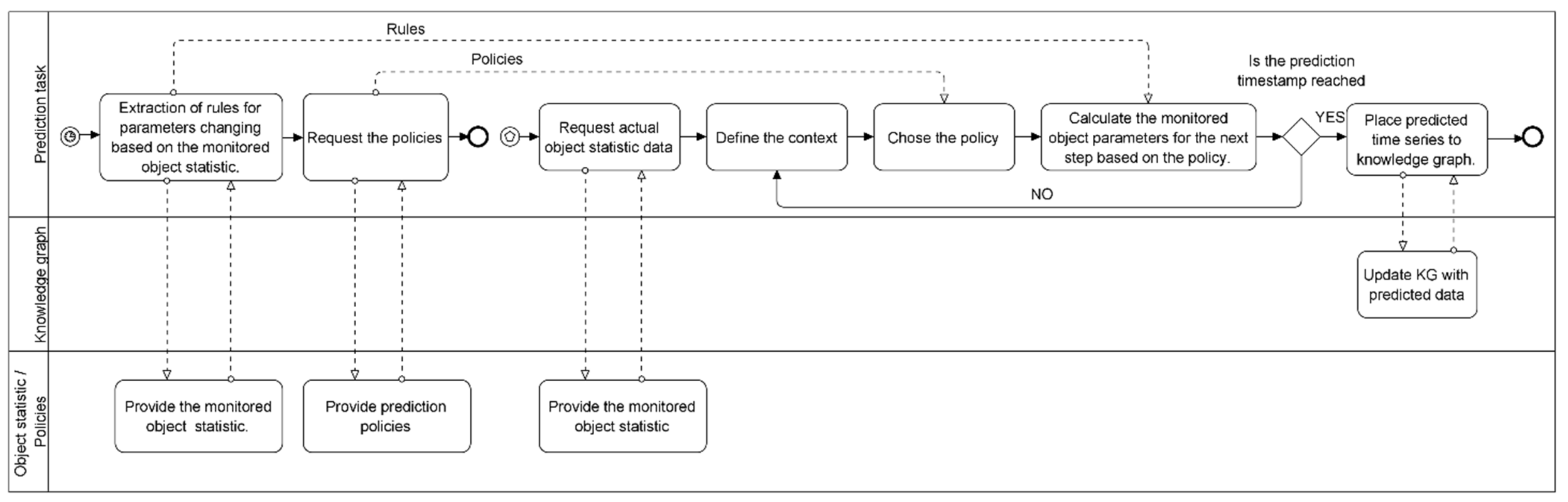
The idea of multilevel adaptive synthesis is that the prediction scheme described in [12] is extended by adding context analysis and the ability to adjust the prediction algorithm at each step. Over time, the state of the object changes, and graph G t k is transformed into graph G t k + T , s k , k + T : G t k G t k + T . Transformation of G t k into G t k + T might be implemented in one step s k s k + 1 or might require a sequence of transformations s k s k + 1 s t k + T 1 s t k + T . Transformation s k , k + 1 consists in the synthesis of G t k + 1 based on G t k . The time step of the synthesis is defined as Δ T = t k + 1 t k .
Possible options for restructuring synthesis processes, depending on the context, are determined by the appointment and use of policies. Each policy is associated with a set of rules for transitions from G t k to G t k + T , according to which, the sets of admissible values of nodes and edges of the model are determined, as well as values for nodes and edges from the sets of their admissible values. As a result of applying the rules, transformations s k s k + 1 are performed.
A conceptual diagram of the multilevel adaptive synthesis is shown in Figure 1.
According to the conceptual diagram, multilevel adaptive synthesis involves the following steps:
  • Determining the policies P ¯ S and rules P for changing the attributes of the model nodes and edges over time depending on the context.
  • Definition of the object model at the current time point t k : G t k based on monitoring system data.
  • Initiation of the model synthesis in one or more steps.
  • Definition of the context (based on the current state of the monitoring object)— S i .
  • Based on the context, choosing a policy P ¯ S i for rebuilding the object model synthesis process on the current step.
  • Transformation execution G t k G t k + 1 . The transformation involves defining the values of the attributes of the nodes and edges of the model.
  • If the target point on the timeline has been reached— t k + T , the task of searching for the predictive model is considered completed and the results of the prediction are recorded to the knowledge graph in the format of time series (the number of elements of the series corresponds to the number of prediction steps).
  • If the target point on the timeline has not been reached— t k + T , the current time is increased according to the prediction period Δ t and the procedure proceeds with step four—definition of the current context.
The context is understood as external operation conditions of the monitoring object, which affect its state. The context is defined through the set of context events— S = S 1 ,   S 2 ,   ,   S Z , at time point t k the context is determined by the context event S i . The context can be described as the ratio of the current context event S i and the state of monitoring object G t k :
C o n t e x t t k = ( S i | G t k ) .
To determine the current context event, one must analyze the values of a given set of parameters of the monitoring object, which act as context metrics [27]. For a formal description of the context metrics, an ontological model of the environment of the monitoring object is used A , which is described as follows: A   O   Q   D   C , where O —the set of the context metrics, Q —the set of the context metrics attributes, D is the set of admissible values for context metrics, C is the set of constraints. Thus, the task of modeling the current situation defined by context can be expressed as follows. Given the specified and formalized knowledge of the monitoring object environment A   O   Q   D   C , it is required to develop a model of the context event S , represented by application context C o n t e x t t = ( S | O p ,   Q p ,   D p ,   C p ,   R p ,   t ) , O p O ,   Q p Q ,   D p D ,   C p C ,   R p R .
When determining the context event based on the analysis of the monitoring object state at time t k , a three-level gradation for the values of the node and edge attributes is proposed.
The entire range of values for the attributes of nodes and edges is divided into three ranges:
  • Green range (corresponds to the normal state of the object. All the object elements are functioning properly);
  • Yellow range (corresponds to the boundary state of the object. It is required to pay attention to the functioning of one or more elements);
  • Red range (faulty state of the object, when it is necessary to urgently take certain actions to return its element or elements to a good state).
This approach allows using a fairly simple algorithm to determine the current context event S i .
The presence of the current context allows rebuilding the synthesis processes of the object models. A policy mechanism is used for rebuilding processes. For the context event S i the policy P ¯ S i is defined as follows: P ¯ S i = p S i , 1 G ¯ S i , t k ,   p S i , 2 G ¯ S i , t k ,   , p S i , W G ¯ S i , t k , where p S i , j G ¯ S i , t k —the rules for the policy P ¯ S i , W —the number of the policy P ¯ S i rules, G ¯ S i , t k —a subset of nodes and edges that a context event can change S i (context metrics). Policies define a set of rules that are based on the statistics of the monitoring object’s functioning or by expert advice, taking into account the context for which the policy is defined.
At each step of the synthesis, to determine the sets of admissible values of nodes and edges of models based on a set of rules P , the following functions are defined: ϕ V ( F V t k , V t k L , E t k H ,   E t k R , C o n t e x t t k ) , ϕ E ( F E t k , V t k L , E t k H ,   E t k R , C o n t e x t t k ) . To determine the values of nodes and edges from the sets of their admissible values, the following functions are constructed ψ V F V t k + 1 ,   V t k L , ψ E H F E t k + 1 ,   E t k H and ψ E R F E t k + 1 ,   E t k R . Using the obtained functional dependencies, the transformation s k s k + 1 is performed.
Thus, the proposed scheme provides the possibility of adaptive synthesis of the processes, of forecasting the state of the observed objects, which makes it possible to solve the forecast problems, taking into account the context determined by their current state.

4. Adaptive Synthesis Method Description

The adaptive synthesis method is designed to transform the model of the monitoring object G t k , describing an object at a point in time t k , into the object model at the moment of time t k + T G t k + T . During the synthesis, the policies P ¯ S are defined, depending on the context as well as the related rules, according to which the synthesis of the object model is performed.
The following are the input data for the adaptive multilevel deductive synthesis method:
  • The time interval at which the synthesis of the model of the monitoring object is performed [ t k ; t k + T ].
  • Synthesis step— Δ t .
  • Model of the monitored object, in which the values of the attributes at the moment t k G t k .
  • Policies used for model transformation s k , k + 1 : P ¯ S .
The output data for the method include the state of the monitoring object and values of its attributes at time t k + T G t k + T .
A formal description of the steps of the multilevel adaptive synthesis method are given below:
  • Get the policies used for synthesis: P ¯ S : P ¯ S 1 ,   P ¯ S 2 ,   ,   P ¯ S Z , where P ¯ S i —the policy related to the context event S i , Z —the number of context events.
  • Obtain actual rules for synthesis of attribute values of model nodes and edges over time: P : P 1 G ,   P 2 G ,   , P N G , where N —the number of attributes.
  • Determine the current state of the object based on the data provided by the monitoring system at the time moment t k . Defining the node and edge attribute values of the monitoring object G t k taking into account the three-level gradation of their values: V i a t r = V i , 1 a t r ,   V i , 2 a t r ,   ,   V i , N a t r , where i —the node identifier, N —the number of nodes, E j a t r = E j , 1 a t r ,   E j , 2 a t r ,   ,   E j , M a t r   , where j —the edge identifier, M—the number of edges.
  • According to the data received from the monitoring system (step 3), or according to the synthesis results in the previous step (step 8), the definition of the context event S i S | G t k .
  • Choose the policy P ¯ S i based on the defined context event S i P ¯ S i = p S i , 1 G ¯ S i , t k ,   p S i , 2 G ¯ S i , t k ,   , p S i , W G ¯ S i , t k   , where P ¯ S i   S i p S i , j G ¯ S i , t k —the rules, connected to the policy, W —the number of rules defined for the policy P ¯ S i , G ¯ S i , t k —a subset of the attributes of nodes and edges, the state of which can change when a context event S i occurs.
  • Using the selected rules, determine the set of acceptable values for nodes and edges at step t k + 1 :
    F V t k + 1 = ϕ V ( FV t k , V t k L , E t k H ,   E t k R , C o n t e x t t k )
    F E t k + 1 = ϕ E ( FE t k , V t k L , E t k H , E t k R , C o n t e x t t k ) ,
    as well as define values for parameters of nodes and edges:
    V t k + 1 L = ψ V ( F V t k + 1 , V t k L )
    E t k + 1 H = ψ E H ( F E t k + 1 , E t k H )
    E t k + 1 R = ψ E R ( F E t k + 1 , E t k R )
  • The model of the monitoring object building at the step t k + 1 : G t k + 1 = V t k + 1 L , E t k + 1 H ,   E t k + 1 R ,   F V t k + 1 ,   F E t k + 1
  • If t k + 1   t k + T , then G t k + 1 = G t k + T —the required model is built, otherwise, set the value t k = t k + 1 and go back to Step 4.

5. Algorithm Description

Figure 2 represents a schematic diagram of the adaptive state prediction algorithm for a complex monitoring object using policies.
The synthesis of the object model is performed in steps, starting from time t k to the time t k + T with the step Δ t .
Diagram description:
Step 1. Setting the initial point in time t k , with reference to which the prediction for the future is made.
Step 2. Request the current state of the monitoring object and attribute values of its nodes and edges G t k ,   G t k a t r .
Step 3. Calculate the set of context metrics O p , t k at time point t k .
The algorithm for step 3 is shown in Figure 3.
The algorithm consists of the following steps:
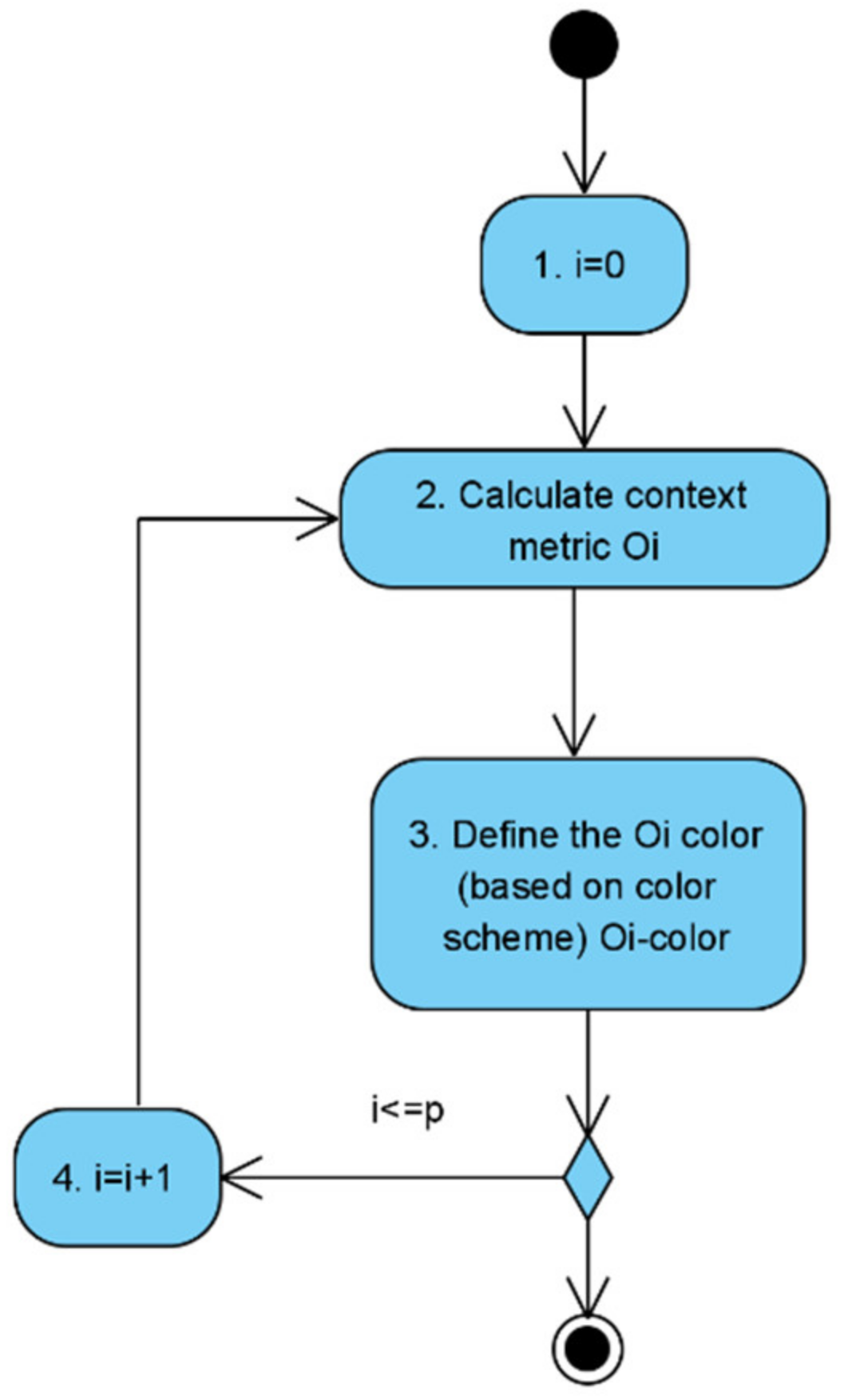
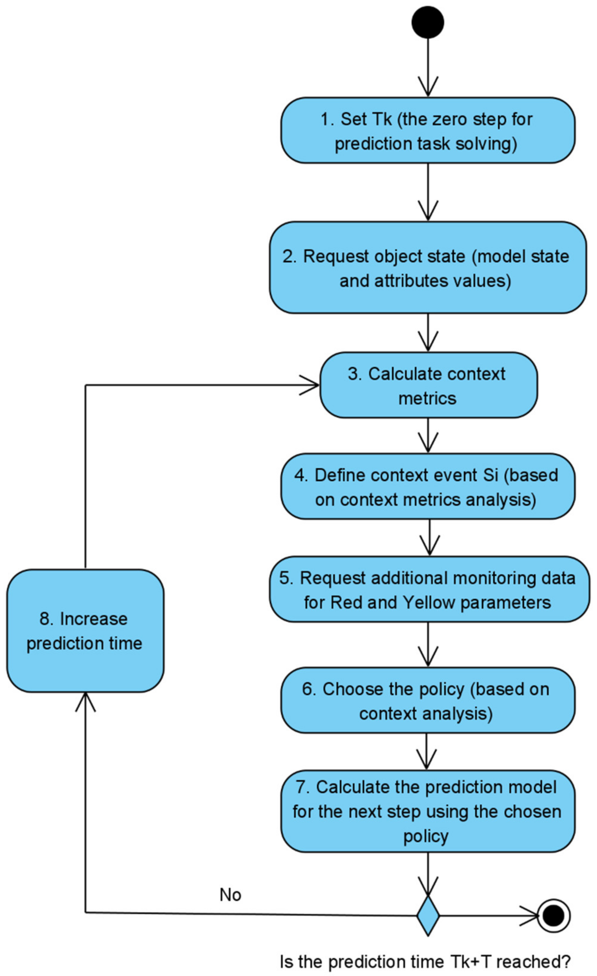
  • The context metrics counter is set to zero: i = 0 .
  • The metric of the context O i is calculated; the metrics of the context are determined through the elements of the model of the monitoring object, the influence is on which context is significant, and by the values, of which it is possible to determine the context of the monitoring object functioning.
  • According to the assigned range of values, the color for the O i context metric is determined:
    • Normal operation (green range);
    • Borderline Operations (yellow range);
    • Abnormal or abnormal operation (red range).
  • If there are unconsidered metrics of the context ( i p ), the counter of the metrics of the context i = i + 1 increases, and a jump to step 2 is performed. Otherwise, it is the end of the algorithm.
Step 4. Determine the context event S i   at time t k (based on the results of calculating the context metrics in step 3).
Step 5. Request additional data on node and edge attribute values at the lower levels of the model for the monitored object parameters that fall within the “Red” and “Yellow” value ranges.
Step 6. Policy P ¯ S i determination is based on the context event S i that has been defined at step 4.
Step 7. Build the monitored object model G t k + 1 .
The algorithm for step 7 is shown in Figure 4.
The algorithm consists of the following steps:
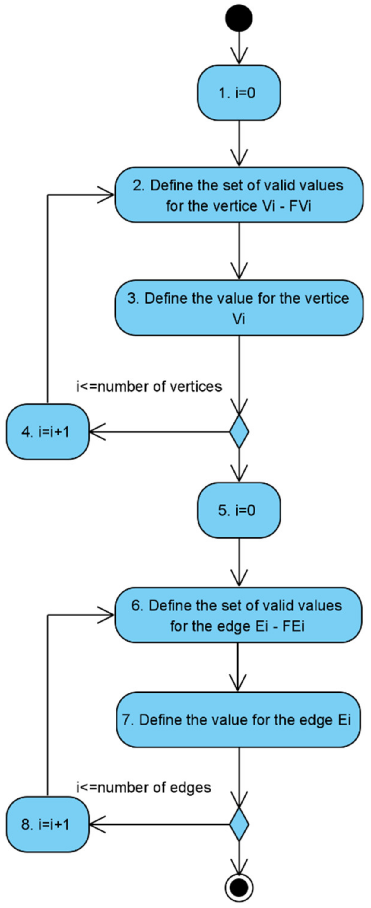
  • The counter of the model nodes is set to zero: i = 0 .
  • The range of valid values for the node V i L is calculated. For this, a rule from the policy P ¯ S i - p S i , V i L G ¯ S i , t k is used.
  • The value for the node V i L is calculated using the function ψ V ( F V i , t k + 1 ,   V i , t k L ) .
  • If there are no considered nodes ( i n o d e s   n u m b e r ), the counter of nodes i = i + 1 increases, and a jump to step 2 is performed. Otherwise, to step 5.
  • The counter of the edges of the model is set to zero: i = 0 .
  • The range of valid values for the edge E i is calculated. For this, a rule from the policy P ¯ S i - p S i , E i G ¯ S i , t k is used.
  • Calculate the value for the edge E i using the function ψ E H F E t k + 1 ,   E t k H or ψ E R F E t k + 1 ,   E t k R depending on the type of edge E i (vertical or horizontal).
  • If there are unconsidered edges ( i e d g e s   n u m b e r ), the counter of edges i = i + 1 is incremented; go to step 6. Otherwise, it is the end of the algorithm.
Step 8. If time point t k + T has not been reached, proceed to the following step; otherwise, complete the synthesis.
Algorithm 1 of the adaptive state prediction method for a complex monitoring object is given below.
Algorithm 1 Adaptive Prediction of Complex Object State Method
//Init
Set t = t k //Set t k —initial current timestamp for prediction algorithm
Set  G t = g e t C u r r e n t S t a t e t //Get initial object state. Description of the function is out of article scope.
Set  G t a t t r = g e t C u r r e n t A t t r t //Get initial attributes values. Description of the function is out of article scope.
//The main prediction cycle t k t k + T  
while ( t t k + T ) {

Set  O p = g e t C o n t e x t M e t r i c s G t ,   G t a t t r //Function for calculating context metrics.
Set  S = g e t C u r r e n t C o n t e x t O p //Function for defining the current context event based on choosing the nearest event in context metrics perspective.

DefineRedYellowParameters( G t ,   G t a t t r ,   G ^ t a t t r ) //Define subsets of the object parameters from Red and Yellow bands— G ^ t a t t r .

Set  G t a t t r a d d i t i o n a l = g e t A d d i t i o n a l A t t r ( G ^ t a t t r ,   t ) //Get additional attributes values. Description of the function is out of article scope.

Set P   = getPolicy(S) //Get policy for the next step processing

Set  G t + Δ T = g e t T h e N e x t S t e p M o d e l P ,   G t //Calculate the object state for the next step
Set  G t + Δ T a t t r = g e t T h e N e x t S t e p A t t r P , G t a t t r ,   G ^ t a t t r //Calculate the attributes values for the next step

Set t = t + Δ T //Go to the next step
}
End

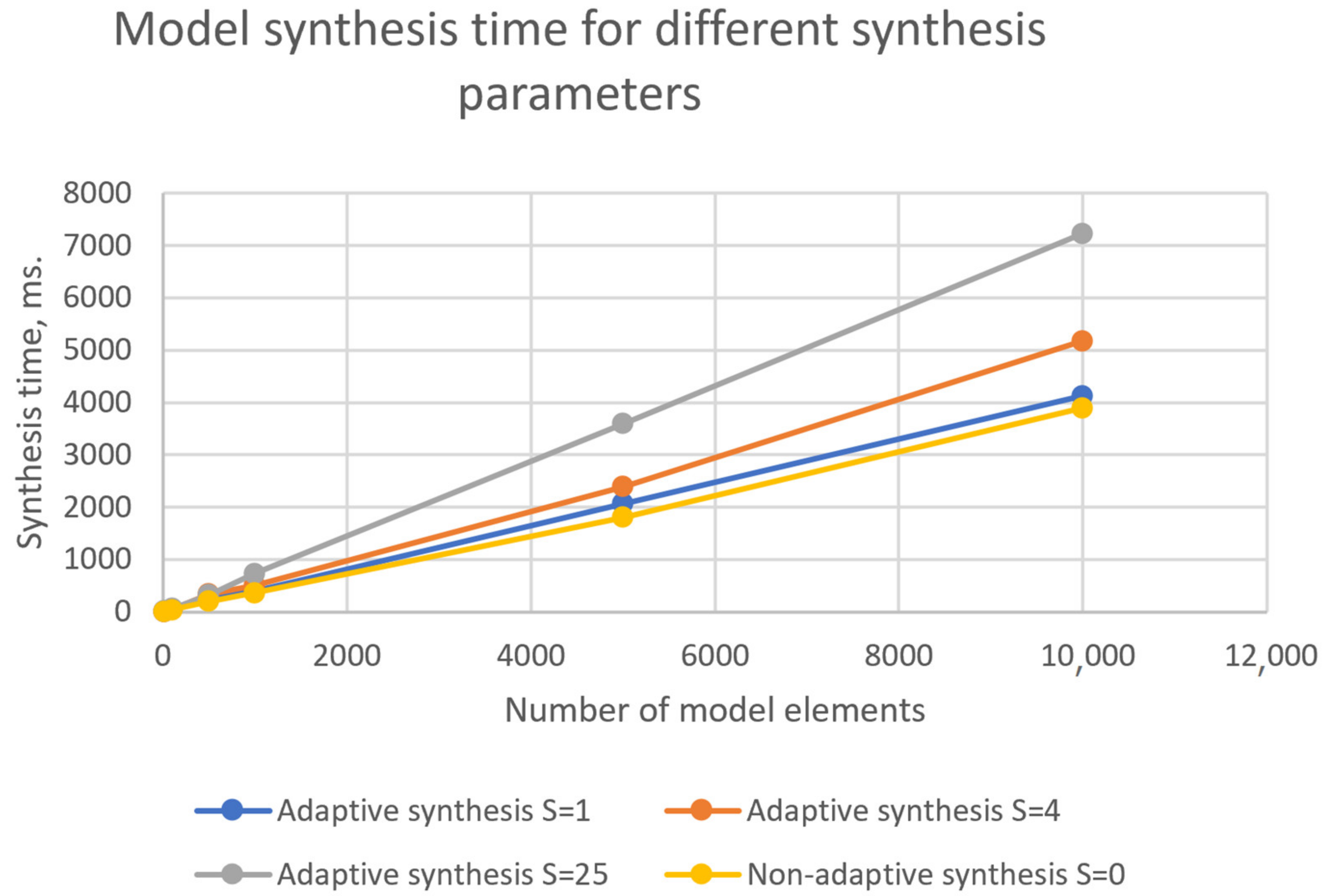
6. Computational Complexity of the Adaptive Multilevel Deductive Synthesis Algorithm

The computational complexity of multilevel deductive synthesis is determined by the number of operations or the time required to build the model. The upper time limit T H is defined as T H c i = 1 K m i 2 , where c is a constant coefficient; m i —the number of problem conditions at the i-th level. The estimate of the lower bound on the time T L for multilevel synthesis is equal to: T L c i = 1 K m i 2 n i 2 .
The computational complexity of adaptive synthesis is higher than non-adaptive due to the need to determine the current context at each step of the synthesis. The graphs of the dependence of the synthesis time on the number of context events, for models with different numbers of elements, are shown in Figure 5.
The figure shows the dependences for the following synthesis parameters:
  • Non-adaptive synthesis (S = 0);
  • Adaptive synthesis, the number of context events S = 1;
  • Adaptive synthesis, the number of context events S = 4;
  • Adaptive synthesis, the number of context events S = 25.
The source code for Python scripts designed to assess the complexity of adaptive synthesis is available in the public GitHub repository [31].

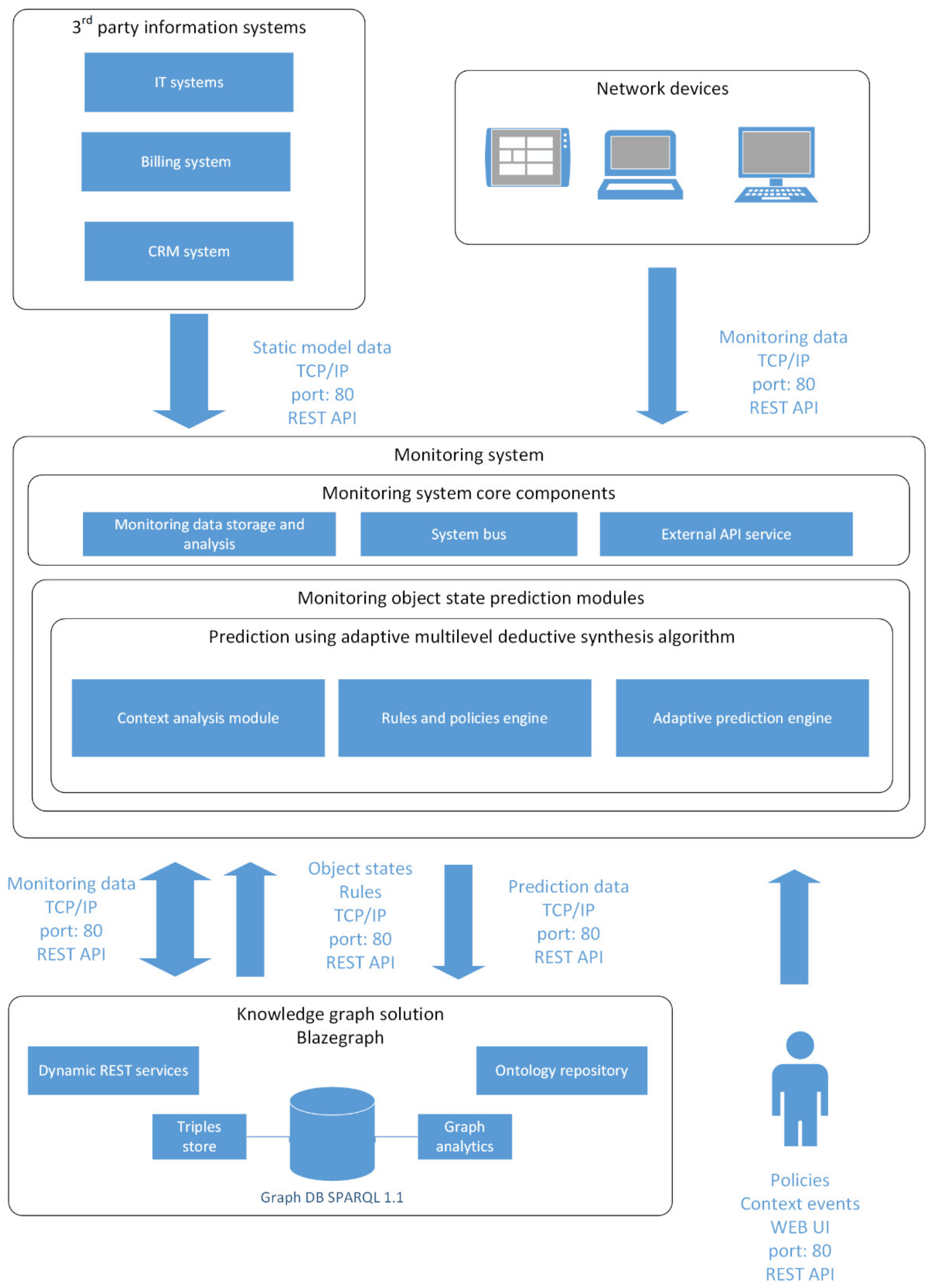
7. The Structure of a Software System for Multilevel Adaptive Synthesis of Object Models

The structure of the developed software system for multilevel adaptive synthesis is shown in Figure 6.
The proposed system consists of the following components.
  • The monitoring system core components, which include:
    • Module of monitoring data storage and analysis.
    • System bus.
    • External API services.
  • Knowledge graph, which includes:
    • SPARQL 1.1 compliant RDF data storage. This component is the key element of the solution holding knowledge graph triples (static and dynamic components), and supporting the functions of adding/removing triples and searching in the RDF storage. The storage also includes a data analytics module. It stores both static and dynamic graph data.
    • An ontology repository that stores replicas of all ontological models of the knowledge graph. It is based on the standards for data and ontology description: RDF [32], RDFS [33], OWL [34].
    • A dynamic REST service that supports API for interaction with external systems, in particular, with the monitoring system core.
  • Operator IT systems, which provide static data for the model. The following operator IT systems are considered:
    • IT system for network infrastructure management that provides data on the network topology, network devices, network services, network applications, accessible data, and access rights.
    • A billing system that provides data on users, their devices, personal accounts, tariffs and payments.
    • CRM systems that provide data on the history of operator-user interaction.
  • The module of prediction using an adaptive multilevel adaptive synthesis algorithm, including:
    • Context analysis module, which allows define the current context event.
    • Rules and policies engine, which is used to define policies and rules for each prediction step.
    • Adaptive prediction engine, which creates prediction nodes in the RDF/XML format and deploys them to the knowledge graph.

8. Case Study

8.1. Task

In order to validate the proposed method, a telecommunication network (TN) was considered as a complex monitoring object. The network is represented as a hierarchy of network devices—routers that accumulate network traffic from user devices. The devices are either stationary or mobile. Mobile devices can move between the coverage areas of different routers. In case the traffic on a router exceeds a threshold value, an emergency situation on the router is defined. The operator has a task to predict the internet traffic on network routers.

8.2. Initial Models of the Monitoring Object

Based on network statistics for routers, stationary, and mobile devices, the rules have been generated in order to assess the traffic. In defining the rules, the following models were used:
  • Model of subscriber devices, describing their state and behavior in terms of hours per day and working/non-working days.
  • Statistical model of the movement of mobile devices between the coverage areas of routers, in terms of hours per day and working/non-working days.
  • Static crash model for routers when the aggregate traffic exceeds the limit.
To assess the state of the routers, the following are defined:
  • Three ranges for the values of the total traffic on the router at a point in time—normal traffic (green zone), increased traffic (yellow zone, when all requests are processed, but there is not enough performance margin), and critical traffic (some or all requests cannot be processed).
  • Three ranges for the number of mobile devices registered on the router at a time—normal number (green zone), increased number (yellow zone, when all requests from devices are processed, but the performance margin is not enough) and critical number (part of requests from devices or all, cannot be processed).

8.3. Proposed Solution

In the considered conditions, the use of only rules for subscriber devices by hours and days cannot provide a reliable forecast, since the movement of user devices and, as a consequence, the possible overload of some routers and the occurrence of emergency situations, must be taken into account. When building a network model, congestion, emergency, and other situations are considered as context events. These events are analyzed at each step of the forecast execution; depending on the events, policies are assigned to predict the state of the object.
The context events are suggested to solve the problem are shown in Table 1:
For every context event, there are policies to predict the internet traffic on the router. The policy descriptions are shown in Table 2.

8.4. Task Solution

The structure of the fragment of the knowledge graph that provides the solution to the task is shown in Figure 7.
For each router at each prediction step, a node in KG tnmo:PredictionNode is specified with the following properties:
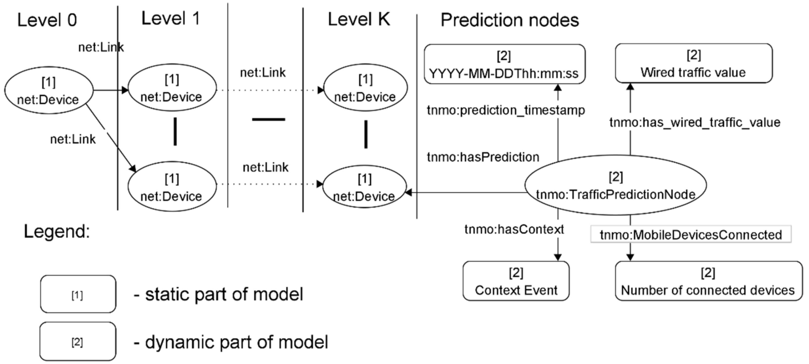
  • tnmo: prediction_timestamp—prediction timestamp;
  • tnmo: has Context—context event that determines which policy is selected for the prediction;
  • tnmo: has_wired_traffic_value—incoming traffic from stationary user devices at the moment of the prediction timestamp;
  • tnmo: MobileDevicesConnected—number of open connections to user mobile network devices.
Thus, the total traffic on the router is determined by adding the traffic from stationary and mobile devices, and it is the value of the total traffic that is analyzed for further color range distribution.
Assumptions and constraints of the experiment:
  • In order to solve the present task, when calculating the traffic from mobile devices—the average daily traffic value of an active mobile device is used. This approach simplifies the implementation of the algorithm and, at the same time, it does not interfere with the achievement of the goals of the experiment being carried out.
  • Only daily rules are used to determine traffic fluctuations and the number of connected devices, as fluctuations within a week will differ only within a day value, depending on the working/non-working day. This limitation does not affect the representativeness of the experiment performed.
  • For the rules, it is assumed that the traffic and the number of connected mobile devices are subject to normal distribution and are set for each time interval by their average values and standard deviations.
For the purpose of computer modeling, the network router hierarchy is restricted to the scheme shown in Figure 8.
Color classification of network traffic, emergency situations, and number of connected devices are shown in Table 3.
The policies described in Table 2 are given in csv format for automated processing as follows:
POLICY_IDRULE_IDACTION
S11aggregation
S21aggregation
S22collection
S31aggregation
S32overload
S33collection
S41aggregation
S42failure
S43collection
A fragment of the daily traffic fluctuation rules and the number of connected devices in csv format is given below:
INTERVAL_IDPARAMETERMEANDEVIATION
00traffic100025
00devices50012
01traffic70011
01devices40050
To solve the task, a Python program has been developed that calculates the necessary predictive components for the knowledge graph in RDF/XML format. These data are then uploaded to the KG and are available for analysis through SPARQL queries. All data are available in a public repository on GitHub [31].
For purposes of the experiment, all of the context events S 1 S 4 described in Table 1 were modeled for the lower-level routers (Figure 8): net: Device_4–net: Device_7. The following SPARQL queries show the results of the experiment (request #1 for normal functioning of the router is listed below. Request #2 for the yellow zone, request #3 for the red zone, and request #4 for router failure are available in the public GitHub repository [31].
Request #1 (normal functioning of router)
PREFIX rdf: <http://www.w3.org/1999/02/22-rdf-syntax-ns#>
PREFIX rdfs: <http://www.w3.org/2000/01/rdf-schema#>
PREFIX net: <http://purl.org/toco/>
Prefix tnmo: <http://127.0.0.1/tnmo#>
SELECT *
WHERE
{
?Predictions tnmo:hasPrediction ?UserDevices.
?Predictions tnmo:prediction_timestamp ?Timestamp.
?Predictions tnmo:has_wired_traffic_value ?Traffic.
?Predictions tnmo:MobileDeviceConnected ?Devices.
?Predictions tnmo:hasContext ?Context.
FILTER(STRSTARTS(?Context, “S1”))
}
LIMIT 2

Response:
PredictionsUserDevicesTimestampTrafficDevicesContext
<http://127.0.0.1/Prediction_1/><http://127.0.0.1/User_device_4/>2021-04-29T01:00:00710.9228508805083329S1/[]
<http://127.0.0.1/Prediction_10/><http://127.0.0.1/User_device_4/>2021-04-29T10:00:00727.330546586905491S1/[]

9. Conclusions

The proposed method of multilevel adaptive synthesis of monitoring objects allows solving the class of problems, of predicting the state of complex objects with variable structures, taking into account the context in which the objects are operating. The tasks are solved by using the mechanism of policies that control the model synthesis processes based on the data coming from the objects. The context is understood as the external conditions of the monitoring object functioning, which influence the state of the object. In this case, context analysis occurs at each step of the synthesis, and depending on a specific event in the context, an appropriate policy is selected for synthesis at the next step. This approach allows adapting the state forecasting algorithm, depending on the current context, which ultimately improves the forecast by taking into account additional objective information. The policies used in the method contain a set of rules generated for each context event. To define the context events, we propose using a three-level color gradation of the values of the attributes of nodes and edges, which simplifies the analysis algorithm and does not interfere with the achievement of the synthesis goal.
The presented example of forecasting the incoming traffic and the number of connected user devices for the routers of the TN demonstrated how the context of the network functioning can be considered, and how it can affect the forecast of the state of the network hubs. As a development of this study, it is advisable to consider the possibility of dynamic reconfiguration of the monitoring object, depending on the context of its functioning, in order to avoid situations of its abnormal operation.

Author Contributions

Conceptualization, K.K. and A.V.; methodology, K.K. and A.V.; software, I.K.; formal analysis, N.Z.; investigation, I.K.; writing—original draft preparation, I.K.; writing—review and editing, N.Z.; visualization, I.K. All authors have read and agreed to the published version of the manuscript.

Funding

This research received no external funding.

Institutional Review Board Statement

Not applicable.

Informed Consent Statement

Not applicable.

Data Availability Statement

The data related to the Case Study section is available in open GitHub repository—https://github.com/kulikovia/INTELS-2021 (accessed on 6 July 2021).

Conflicts of Interest

The authors declare no conflict of interest.

References

  1. Kotseruba, I.; Tsotsos, J.K. 40 years of cognitive architectures: Core cognitive abilities and practical applications. Artif. Intell. Rev. 2018, 52, 1–78. [Google Scholar] [CrossRef] [Green Version]
  2. Osipov, V.; Nikiforov, V.; Zhukova, N.; Miloserdov, D. Urban traffic flows forecasting by recurrent neural networks with spiral structures of layers. Neural Comput. Applic. 2020, 32, 14885–14897. [Google Scholar] [CrossRef]
  3. Osipov, V.; Lushnov, M.; Stankova, E.; Vodyaho, A.; Shichkina, Y.; Zhukova, N. Automatic Synthesis of Multilevel Automata Models of Biological Objects. In Proceedings of the International Conference on Computational Science and Its Applications (ICCSA 2019), Saint Petersburg, Russia, 1–4 July 2019; Springer: Cham, Switzerland, 2019; pp. 441–456. [Google Scholar]
  4. Osipov, V.; Vodyaho, A.; Zhukova, N.; Glebovsky, P. Multilevel Automatic Synthesis of Behavioral Programs for Smart Devices. In Proceedings of the Control, Artificial Intelligence, Robotics & Optimization (ICCAIRO 2017), Prague, Czech Republic, 20–22 May 2017; pp. 335–340. [Google Scholar]
  5. Cardoso, S.D.; da Silveira, M.; Pruski, C. Construction and exploitation of an historical knowledge graph to deal with the evolution of ontologies. Knowl. Based Syst. 2020, 194, 105508. [Google Scholar] [CrossRef]
  6. Malik, K.M.; Krishnamurthy, M.; Alobaidi, M.; Hussain, M.; Alam, F.; Malik, G. Automated domain-specific healthcare knowledge graph curation framework: Subarachnoid hemorrhage as phenotype. Expert Syst. Appl. 2020, 145, 113120. [Google Scholar] [CrossRef]
  7. Liang, Y.; Xu, F.; Zhang, S.H.; Lai, Y.-K.; Mu, T. Knowledge graph construction with structure and parameter learning for indoor scene design. Comp. Vis. Media 2018, 4, 123–137. [Google Scholar] [CrossRef] [Green Version]
  8. Martinez-Rodriguez, J.L.; Lopez-Arevalo, I.; Rios-Alvarado, A.B. OpenIE-based approach for Knowledge Graph construction from text. Expert Syst. Appl. 2018, 113, 339–355. [Google Scholar] [CrossRef]
  9. Nguyen, H.L.; Jung, J.J. Social event decomposition for constructing knowledge graph. Future Gener. Comput. Syst. 2019, 100, 10–18. [Google Scholar] [CrossRef]
  10. Krinkin, K.; Vodyaho, A.; Kulikov, I.; Zhukova, N. Models of Telecommunications Network Monitoring Based on Knowledge Graphs. In Proceedings of the 9th Mediterranean Conference on Embedded Computing (MECO), Budva, Montenegro, 8–11 June 2020; pp. 1–7. [Google Scholar] [CrossRef]
  11. Kulikov, I.; Wohlgenannt, G.; Shichkina, Y.; Zhukova, N. An Analytical Computing Infrastructure for Monitoring Dynamic Networks Based on Knowledge Graphs. In Lecture Notes in Computer Science, Proceedings of the Computational Science and Its Applications–ICCSA 2020, Caligary, Italy, 1–4 July 2020; Gervasi, O., Murgante, B., Misra, S., Garau, C., Blečić, I., Taniar, D., Apduhan, B.O., Rocha, A.M.A.C., Tarantino, E., Torre, C.M., et al., Eds.; Springer: Cham, Switzerland, 2020; Volume 12254. [Google Scholar] [CrossRef]
  12. Krinkin, K.; Kulikov, I.; Vodyaho, A.; Zhukova, N. Prediction of Telecommunication Network State Based on Knowledge Graphs. In Proceedings of the 28th Conference of Open Innovations Association (FRUCT), Moscow, Russia, 27–29 January 2021; pp. 200–207. [Google Scholar] [CrossRef]
  13. Long, J.; Chen, Z.; He, W.; Wu, T.; Ren, J. An integrated framework of deep learning and knowledge graph for prediction of stock price trend: An application in Chinese stock exchange market. Appl. Soft Comput. 2020, 91, 106205. [Google Scholar] [CrossRef]
  14. Mao, Q.; Li, X.; Peng, H.; Li, J.; He, D.; Guo, S.; He, M.; Wang, L. Event prediction based on evolutionary event ontology knowledge. Future Gener. Comput. Syst. 2021, 115, 76–89. [Google Scholar] [CrossRef]
  15. Tempelmeier, N.; Demidova, E. Linking OpenStreetMap with knowledge graphs—Link discovery for schema-agnostic volunteered geographic information. Future Gener. Comput. Syst. 2021, 116, 349–364. [Google Scholar] [CrossRef]
  16. Shi, D.; Wang, T.; Xing, H.; Xu, H. A learning path recommendation model based on a multidimensional knowledge graph framework for e-learning. Knowl. Based Syst. 2020, 195, 105618. [Google Scholar] [CrossRef]
  17. Lu, W.; Altenbek, G. A recommendation algorithm based on fine-grained feature analysis. Expert Syst. Appl. 2021, 163, 113759. [Google Scholar] [CrossRef]
  18. Shao, B.; Li, X.; Bian, G. A survey of research hotspots and frontier trends of recommendation systems from the perspective of knowledge graph. Expert Syst. Appl. 2021, 165, 113764. [Google Scholar] [CrossRef]
  19. Wang, H.; Wang, Z.; Hu, S.; Xu, X.; Chen, S.; Tu, Z. DUSKG: A fine-grained knowledge graph for effective personalized service recommendation. Future Gener. Comput. Syst. 2019, 100, 600–617. [Google Scholar] [CrossRef]
  20. Yang, Z.; Dong, S. HAGERec: Hierarchical Attention Graph Convolutional Network Incorporating Knowledge Graph for Explainable Recommendation. Knowl. Based Syst. 2020, 204, 106194. [Google Scholar] [CrossRef]
  21. Sang, L.; Xu, M.; Qian, S.; Wu, X. Knowledge graph enhanced neural collaborative recommendation. Expert Syst. Appl. 2021, 164, 113992. [Google Scholar] [CrossRef]
  22. Tianxing, M.; Osipov, V.Y.; Vodyaho, A.I.; Kalmatskiy, A.; Zhukova, N.A.; Lebedev, S.V.; Shichkina, Y.A. Reconfigurable monitoring for telecommunication networks. PeerJ Comput. Sci. 2020, 6. [Google Scholar] [CrossRef] [PubMed]
  23. Zhukova, N.A. General and Specific Problems of Multilevel Synthesis of Models of Monitoring Objects. Autom. Doc. Math. Linguist. 2019, 53, 315–321. [Google Scholar] [CrossRef]
  24. Vert, G.; Iyengar, S.S.; Phoha, V.V. Introduction to Contextual Processing: Theory and Applications, 1st ed.; Chapman and Hall/CRC: Boca Raton, FL, USA, 2010. [Google Scholar] [CrossRef]
  25. Serrano, J.M. Applied Ontology Engineering in Cloud Services, Networks and Management Systems; Springer: New York, NY, USA, 2012; Available online: https://books.google.ru/books?id=X8ZBiRXwV0gC (accessed on 5 July 2021).
  26. Brézillon, P.; Pomerol, J.-C. Contextual knowledge and proceduralized context. In Proceedings of the AAAI Workshop on Modeling Context in AI Applications, Orlando, FL, USA, July 18–19; pp. 16–20, ⟨hal-01574756⟩.
  27. Smirnov, A.V.; Pashkin, M.P.; Shilov, N.G.; Levashova, T.V.; Kashevnik, A.M. Context-aware decision support in distributed information environment. Informatsionnye Tekhnologii i Vychslitel’nye Sistemy 2009, 38–48. [Google Scholar]
  28. Liu, H.; Gegov, A.; Haig, E. Rule Based Systems for Big Data: A Machine Learning Approach; Springer: Cham, Switzerland, 2016. [Google Scholar] [CrossRef] [Green Version]
  29. Bellini, P.; Nesi, P. Performance assessment of RDF graph databases for smart city services. J. Vis. Lang. Comput. 2018, 45, 24–38. [Google Scholar] [CrossRef]
  30. Bizer, C.; Schultz, A. The Berlin SPARQL benchmark. Int. J. Semant. Web Inf. Syst. 2009, 5, 1–24. [Google Scholar] [CrossRef] [Green Version]
  31. GitHub Repository. Available online: https://github.com/kulikovia/INTELS-2021 (accessed on 5 July 2021).
  32. RDF. Available online: https://www.w3.org/RDF (accessed on 5 July 2021).
  33. RDFS. Available online: https://www.w3.org/TR/rdf-schema (accessed on 5 July 2021).
  34. OWL. Available online: https://www.w3.org/OWL (accessed on 5 July 2021).
Figure 1. Conceptual diagram of the multilevel adaptive synthesis.
Applsci 11 06251 g001
Figure 2. Conceptual diagram of the multilevel adaptive synthesis.
Applsci 11 06251 g002
Figure 3. Scheme of the algorithm for determining the context metrics.
Applsci 11 06251 g003
Figure 4. Diagram of the algorithm for predicting the state of the monitoring object for every step.
Applsci 11 06251 g004
Figure 5. The time dependence of adaptive and non-adaptive synthesis of object models depending on the number of possible context events.
Applsci 11 06251 g005
Figure 6. The structure of the software system for multilevel adaptive synthesis of the knowledge graph of the monitoring object.
Applsci 11 06251 g006
Figure 7. The structure of the software system for multilevel adaptive synthesis of the knowledge graph of the monitoring object.
Applsci 11 06251 g007
Figure 8. Network router hierarchy.
Applsci 11 06251 g008
Table 1. Context events.
Context EventDescriptionAssessment Parameters for the Monitoring System Side
S 1 Normal operationTraffic—green zone
Number of registered mobile devices—green zone
Emergency situation—no
S 2 Increased loadTraffic—yellow zone
Number of registered mobile devices—yellow zone
Emergency situation—no
S 3 OverloadTraffic—red zone (below the threshold value)
Number of registered mobile devices—yellow or red zone
Emergency situation—no
S 4 EmergencyTraffic—red zone (above the threshold value)
Number of registered mobile devices—any value
Emergency situation—yes
Table 2. Policy description.
PolicyPolicy Description
P ¯ 1 | S 1 Rule 1: Aggregate traffic from devices according to hourly/daily rules. No additional operations are required.
P ¯ 2 | S 2 Rule 1: Aggregate traffic from devices according to hourly/daily rules.
Rule 2: Receive additional monitoring parameters from devices that are at the lower levels of the hierarchy and record these parameters in the monitoring system.
P ¯ 3 | S 3 Rule 1: Aggregate traffic from devices according to hourly/daily rules.
Rule 2: Record network overload state. Part of the requests from user devices will not be processed by the system. Traffic and number of connected devices will be restricted to the lower limit of the red zone.
Rule 3: Receive additional monitoring parameters from devices that are at the lower levels of the hierarchy and record these parameters in the monitoring system.
P ¯ 4 | S 4 Rule 1: Aggregate traffic from devices according to hourly/daily rules.
Rule 2: Record the emergency situation on the router. Reset the traffic and the number of connected devices if the emergency limit is exceeded.
Rule 3: Receive additional monitoring parameters from devices that are at the lower levels of the hierarchy and record these parameters in the monitoring system.
Table 3. Color classification of parameter values.
ParameterGreen ZoneYellow ZoneRed Zone
Incoming traffic0–0.8 Gb/s0.8–1.0 Gb/s1.0–1.5 Gb/s
Number of open connections to mobile devices 0–500500–800800–850
Emergency situationIncoming traffic > 1.5 Gb/s
Number of open connections to mobile devices > 850
Publisher’s Note: MDPI stays neutral with regard to jurisdictional claims in published maps and institutional affiliations.

