Statistical Hypothesis Testing for Asymmetric Tolerance Index

Abstract

Many of the nominal-the-best quality characteristics of important machine tool components, such as inner or outer diameters, have asymmetric tolerances. An asymmetric tolerance index is a function for the average of the process and the standard deviation. Unfortunately, it is difficult to obtain the $100\left(1-\alpha \right)\%$ confidence interval of the index. Therefore, this study adopts Boole’s inequality and DeMorgan’s theorem to find the combined confidence region for the average of the process as well as the standard deviation. Next, using the asymmetric tolerance index for the target function and the combined confidence region for the feasible region, this study applies mathematical programming to find the confidence interval as well as employs this confidence interval for statistical hypothesis testing. Lastly, this study demonstrates the applicability of the proposed approach with an illustrative example.

1. Introduction

Taiwan’s machine tool industry’s output value and export volume are second to none in the world. Central Taiwan in particular is home to a large machine tool and machinery industry cluster incorporating the aerospace industry and the smart machinery industry. It includes several mechanical processing plants for precision machinery, machine tools, and important components [1,2,3]. Prahalad and Hamel [4] and Grossman and Helpman [5] pointed out that more and more companies were outsourcing their non-core operations to manufacturers specializing in the aforementioned areas to cut down on operating costs, focus their resources on their core technologies, and enhance not only their efficiency but also their competitiveness. In this context, the machine tool industry’s clustering effect in Central Taiwan has resulted in a local supply chain that plays an important role in the global market.

Many of the nominal-the-best quality characteristics (QCs) of important machine tool components, such as the inner or outer diameters of shafts, bearings, and gears, have asymmetric tolerances [6,7,8,9]. A process capability index (PCI) is not only a convenient tool for process capability assessment and analysis but also an effective tool for communication between sales departments and customers [10,11,12,13,14,15,16]. A process has a symmetric tolerance when the target value, T, equals the tolerance midpoint, M, where M $=$ $(USL+LSL)/2$, and $USL$ and $LSL$ are the upper and lower specification limits, respectively. Suppose that $X$ should be the quality characteristic of a process followed by an ordinary allocation using the average value of $\mu$ and the standard deviation of $\sigma$ (i.e., $X~N\left(\mu ,{\sigma }^2\right)$). Based on this assumption, Kane [17] proposed capability index $C_{PK}$ on the basis of the process yield with symmetric tolerance:

$$C_{PK}=Min\left\{\frac{USL-\mu }{3\sigma },\frac{\mu -LSL}{3\sigma }\right\}=\frac{1-\left|{\delta }^{\prime }\right|}{3{\gamma }^{\prime }},$$

(1)

where $d^{\prime }$ $=$ $(USL-LSL)/2$, ${\delta }^{\prime }=\left(\mu -T\right)/d^{\prime }$, and ${\gamma }^{\prime }=\sigma /d^{\prime }$. According to Boyles [18], the relation between index $C_{PK}$ and the process yield can be shown as follows:

$$2\Phi \left(3C_{pk}\right)-1 \le Yield\%<\Phi \left(3C_{pk}\right)$$

(2)

In Equation (2), $\Phi (\cdot )$ refers to the function of cumulative distribution for the ordinary allocation. As mentioned above, the quality characteristics of many machinery products have asymmetric tolerances. A process has asymmetric tolerances when $D_u$ $=$ $USL-T$ does not equal $D_l$ $=$ $T-LSL$ (T ≠ M), where $D_u$ is the upper tolerance and $D_l$ is the lower tolerance. If d $=$ $Min\left\{D_u,D_l\right\}$, $d_u=d/D_u$, and $d_l=d/D_l$, then the process capability index containing asymmetric tolerances suggested by Pearn and Chen [19] can be defined as follows:

$$C_{PK}^{″}=\frac{d-Max\left\{d\left(\mu -T\right)/D_u,d\left(T-\mu \right)/D_l\right\}}{3\sigma }=\frac{d-Max\left\{d_u\left(\mu -T\right),d_l\left(T-\mu \right)\right\}}{3\sigma }.$$

(3)

Obviously, when T $=$ M (a symmetric case), then $C_{PK}^{″}$ $=$ $C_{PK}$.

Asymmetric tolerance index $C_{PK}^{″}$ is a function of $\mu$ and $\sigma$, which means it simultaneously depends on $\mu$ and $\sigma$. Unfortunately, the sampling distribution of index $C_{PK}^{″}$ is complex, making its $100\left(1-\alpha \right)\%$ confidence interval hard to derive. As a result, this study adopts Boole’s Inequality and DeMorgan’s Theorem to find the combined confidence zone of $\left(\mu ,\sigma \right)$. Next, using index $C_{pk}^{″}$ for the target function and the confidence zone of $\left(\mu ,\sigma \right)$ for the feasible zone, this study applies mathematical programming to find the confidence interval of index $C_{PK}^{″}$ and employs this for statistical hypothesis testing capabilities of QCs with asymmetric tolerances meeting required quality levels. To sum up, the advantages of the model proposed in this study are that it (1) assesses the process quality of the asymmetric tolerance and symmetrical tolerance products; (2) uses mathematic programming to deduce confidence interval easily without regarding the complicated distribution of the estimated formula of the estimator of index $C_{PK}^{″}$; (3) reduces the misjudgment risk of sampling error owing to testing through the confidence interval.

The other sections of this study are arranged as follows: Section 2 displays the $100\left(1-\alpha \right)\%$ confidence interval of the asymmetric tolerance index $C_{PK}^{″}$, Section 3 demonstrates the $100\left(1-\alpha \right)\%$ confidence interval used to construct statistical testing rules, Section 4 provides an illustrative example to explain the applicability of the method proposed by this study, and Section 5 presents conclusions. A conceptual framework of the Introduction section is shown in Figure 1.

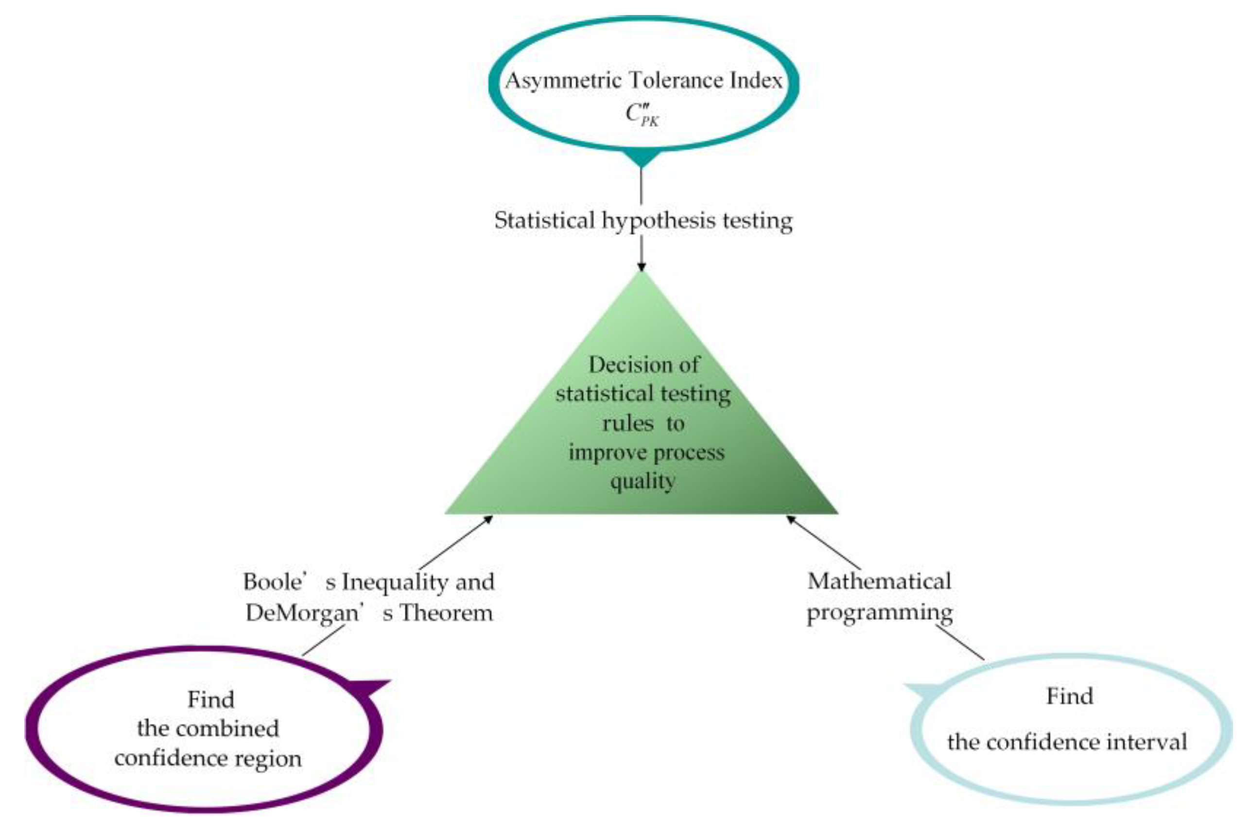
2. Confidence Region

The section we will displays the $100\left(1-\alpha \right)\%$ confidence interval of the asymmetric tolerance index $C_{PK}^{″}$ by Boole’s inequality and DeMorgan’s theorem.

First, $X_1,X_2,\dots ,X_n$ is assumed as a randomly chosen sample of $N\left(\mu ,{\sigma }^2\right)$. Both the mean and variance of the sample are expressed in the following equations:

$$\overline{X}=\frac{1}{n}{\displaystyle {\sum }_{i=1}^n{X}_i},$$

(4)

$$S=\sqrt{\frac{1}{n-1}{\displaystyle {\sum }_{i=1}^n{\left(X_i-\overline{X}\right)}^2}}.$$

(5)

Furthermore, we let

$$T=\frac{\sqrt{n}\left(\overline{X}-\mu \right)}{S},$$

(6)

$$K=\frac{\left(n-1\right)S^2}{{\sigma }^2},$$

(7)

where $T$ and $K$ are respectively allotted as $t_{n-1}$ and ${\chi }_{n-1}^2$. To receive the $\left(1-\alpha \right)\times 100\%$ lower confidence limits on index $C_{pk}^{″}$, events $E_{\delta }$ and $E_{\gamma }$ are defined as follows:

$$E_{\delta }=\left\{S-e_t\le T\le S+e_t\right\}$$

(8)

and

$$E_{\gamma }=\left\{{\chi }_{\alpha /4;n-1}^2\le K\le {\chi }_{1-\alpha /4;n-1}^2\right\},$$

(9)

where

$$e_t=t_{\alpha /4;n-1}\times \left(\frac{S}{\sqrt{n}}\right),$$

(10)

$t_{\alpha /4;n-1}$ is the upper $\alpha /4$ quantile of $t_{n-1}$, ${\chi }_{\alpha /4;n-1}^2$ is the upper $\alpha /4$ quantile of ${\chi }_{n-1}^2$, and $\alpha$ stands for the confidence level. Clearly, $P\left(E_{\delta }\right)=P\left(E_{\gamma }\right)=1-\left(\alpha /2\right)$, so $P\left(E_{\delta }^C\right)=P\left(E_{\gamma }^C\right)=\alpha /2$. Considering Boole’s inequality and DeMorgan’s theorem, $P\left(E_{\delta }\cap E_{\gamma }\right)\ge 1-P\left(E_{\delta }^C\right)-P\left(E_{\gamma }^C\right)$ is derived. Therefore,

$$p\left\{{\widehat{\delta }}^{*}-e_t\le T\le {\widehat{\delta }}^{*}+e_t,{\chi }_{\alpha /4;n-1}^2\le K\le {\chi }_{1-\alpha /4;n-1}^2\right\}=1-\alpha .$$

(11)

Equivalently,

$$P\left\{\overline{X}-t_{\alpha /4;n-1}\times \left(\frac{S}{\sqrt{n}}\right)\le \mu \le \overline{X}+t_{\alpha /4;n-1}\times \left(\frac{S}{\sqrt{n}}\right),\sqrt{\frac{n-1}{{\chi }_{1-\alpha /4;n-1}^2}}S\le \sigma \le \sqrt{\frac{n-1}{{\chi }_{\alpha /4;n-1}^2}}S\right\}=1-\alpha .$$

(12)

If we let $(x_1,x_2,\dots x_n)$ be the observed values of $(X_1,X_2,\dots X_n)$, then $\overline{x}$ and $s$ are expressed as the observed values of $\overline{X}$ and $S$, respectively, below:

$$\overline{x}=\frac{1}{n}{\displaystyle \sum _{i=1}^n{x}_i},$$

(13)

$$s=\sqrt{\frac{1}{n}{\displaystyle \sum _{i=1}^n{\left(x_i-\overline{x}\right)}^2}}.$$

(14)

Therefore, the confidence region is expressed as follows:

$$CR=\left\{\left(\mu ,\sigma \right)|\overline{x}-e_{t0}\le \mu \le \overline{x}+e_{t0},\sqrt{\frac{n-1}{{\chi }_{1-\alpha /4;n-1}^2}}s\le \sigma \le \sqrt{\frac{n-1}{{\chi }_{\alpha /4;n-1}^2}}s\right\}$$

(15)

where $e_{t0}$ is the observed value of $e_t$ and is written below:

$$e_{t0}=t_{\alpha /4;n-1}\times \left(\frac{s}{\sqrt{n}}\right).$$

(16)

Clearly, $C_{pk}^{″}$ represents the function of $\left(\mu ,\sigma \right)$. According to Chen et al. [20], we can employ mathematical programming to receive the lower confidence limit $L{C}_{pk}^{″}$ from $C_{pk}^{″}$ and the upper confidence limit $U{C}_{pk}^{″}$ from $C_{pk}^{″}$. $C_{pk}^{″}$ refers to the target function, while the confidence region (CR) is viewed as the feasible region, as shown below:

$$\{\begin{array}{l}L{C}_{pk}^{″}=Min C_{pk}^{″}\\ s.t.\left(\mu ,\sigma \right)\in CR\end{array}$$

(17)

and

$$\{\begin{array}{l}U{C}_{pk}^{″}=Max C_{pk}^{″}\\ s.t.\left(\mu ,\sigma \right)\in CR\end{array}.$$

(18)

Next, we discuss three cases: (1) T $\in$ $\left[\overline{x}-e_{t0},\overline{x}+e_{t0}\right]$, (2) $\overline{x}-e_{t0}$ $>$T, and (3) $\overline{x}+e_{t0}$ $<$ T.

Case 1: T $\in$ $\left[\overline{x}-e_{t0},\overline{x}+e_{t0}\right]$

In case 1, we can conclude that since $\mu$ $=$ T and $C_{pk}^{″}=d/(3\sigma )$, then

$${\hat{C}}_{pk0}^{″}=\frac{d}{3s}$$

(19)

where ${\hat{C}}_{pk0}^{″}$ represents the observed values of ${\hat{C}}_{pk}^{″}$. Furthermore, the confidence region is expressed as

$$CR=\left\{\left(\mu ,\sigma \right)|\mu =T,\sqrt{\frac{n-1}{{\chi }_{1-\alpha /4;n-1}^2}}s\le \sigma \le \sqrt{\frac{n-1}{{\chi }_{\alpha /4;n-1}^2}}s\right\}.$$

(20)

Then the mathematical programming model is illustrated below:

$$0\{\begin{array}{l}L{C}_{pk}^{″}=Min \frac{d}{3\sigma }\\ subject to\\ \sqrt{\frac{n-1}{{\chi }_{1-\alpha /4;n-1}^2}}s\le \sigma \le \sqrt{\frac{n-1}{{\chi }_{\alpha /4;n-1}^2}}s\end{array} \mathrm{and} \{\begin{array}{l}U{C}_{pk}^{″}=Max \frac{d}{3\sigma }\\ subject to\\ \sqrt{\frac{n-1}{{\chi }_{1-\alpha /4;n-1}^2}}s\le \sigma \le \sqrt{\frac{n-1}{{\chi }_{\alpha /4;n-1}^2}}s\end{array}.$$

Obviously, the $100\left(1-\alpha \right)\%$ confidence interval of $C_{pk}^{″}$ is

$$\left[L{C}_{pk}^{″},U{C}_{pk}^{″}\right]=\left[{\hat{C}}_{pk0}^{″}\times \frac{\sqrt{{\chi }_{\alpha /4;n-1}^2}}{\sqrt{n-1}},{\hat{C}}_{pk0}^{″}\times \frac{\sqrt{{\chi }_{1-\alpha /4;n-1}^2}}{\sqrt{n-1}}\right].$$

(21)

Case 2: $\overline{x}-e_{t0}$ $>$ T

In case 2, it is concluded that when $\mu$ $>$ T, then

$$C_{pk}^{″}=\frac{d-d_u\left(\mu -T\right)}{3\sigma },$$

(22)

$${\hat{C}}_{pk0}^{″}=\frac{d-d_u\left(\overline{x}-T\right)}{3s}.$$

(23)

Similar to case 1, the mathematical programming model is exhibited below:

$$\{\begin{array}{l}L{C}_{pk}^{″}=Min \frac{d-d_u\left(\mu -T\right)}{3\sigma }\\ subject to\\ \overline{x}-e_{t0}\le \mu \le \overline{x}+e_{t0}\\ \sqrt{\frac{n-1}{{\chi }_{1-\alpha /4;n-1}^2}}s\le \sigma \le \sqrt{\frac{n-1}{{\chi }_{\alpha /4;n-1}^2}}s\end{array} \mathrm{and} \{\begin{array}{l}U{C}_{pk}^{″}=Max \frac{d-d_u\left(\mu -T\right)}{3\sigma }\\ subject to\\ \overline{x}-e_{t0}\le \mu \le \overline{x}+e_{t0}\\ \sqrt{\frac{n-1}{{\chi }_{1-\alpha /4;n-1}^2}}s\le \sigma \le \sqrt{\frac{n-1}{{\chi }_{\alpha /4;n-1}^2}}s\end{array}$$

Obviously, $\left[L{C}_{pk}^{″},U{C}_{pk}^{″}\right]$ is the $100\left(1-\alpha \right)\%$ confidence interval of $C_{pk}^{″}$, where

$$L{C}_{pk}^{″}=\frac{d-d_u\left(\overline{x}-T+t_{\alpha /4;n-1}\times \frac{s}{\sqrt{n}}\right)}{3\sqrt{\frac{n-1}{{\chi }_{\alpha /4;n-1}^2}}s}=\left({\hat{C}}_{pk0}^{″}-\frac{d_u{t}_{\alpha /4;n-1}}{3\sqrt{n}}\right)\times \sqrt{\frac{{\chi }_{\alpha /4;n-1}^2}{n-1}},$$

(24)

$$U{C}_{pk}^{″}=\frac{d-d_u\left(\overline{x}-T-t_{\alpha /4;n-1}\times \frac{s}{\sqrt{n}}\right)}{3\sqrt{\frac{n-1}{{\chi }_{1-\alpha /4;n-1}^2}}s}=\left({\hat{C}}_{pk0}^{″}+\frac{d_u{t}_{\alpha /4;n-1}}{3\sqrt{n}}\right)\times \sqrt{\frac{{\chi }_{1-\alpha /4;n-1}^2}{n-1}}.$$

(25)

Case 3: $\overline{x}+e_{t0}$ $<$ T

In case 3, we can conclude that since $\mu$ $<$ T, then

$$C_{pk}^{″}=\frac{d+d_l\left(\mu -T\right)}{3\sigma },$$

(26)

$${\hat{C}}_{pk0}^{″}=\frac{d+d_l\left(\overline{x}-T\right)}{3s}.$$

(27)

Therefore, the mathematical programming model is demonstrated below:

$$\{\begin{array}{l}L{C}_{pk}^{″}=Min \frac{d+d_l\left(\mu -T\right)}{3\sigma }\\ subject to\\ \overline{x}-e_{t0}\le \mu \le \overline{x}+e_{t0}\\ \sqrt{\frac{n-1}{{\chi }_{1-\alpha /4;n-1}^2}}s\le \sigma \le \sqrt{\frac{n-1}{{\chi }_{\alpha /4;n-1}^2}}s\end{array} \mathrm{and} \{\begin{array}{l}U{C}_{pk}^{″}=Max \frac{d+d_l\left(\mu -T\right)}{3\sigma }\\ subject to\\ \overline{x}-e_{t0}\le \mu \le \overline{x}+e_{t0}\\ \sqrt{\frac{n-1}{{\chi }_{1-\alpha /4;n-1}^2}}s\le \sigma \le \sqrt{\frac{n-1}{{\chi }_{\alpha /4;n-1}^2}}s\end{array}$$

Obviously, $\left[L{C}_{pk}^{″},U{C}_{pk}^{″}\right]$ is the $100\left(1-\alpha \right)\%$ confidence interval of $C_{pk}^{″}$, where

$$L{C}_{pk}^{″}=\frac{d+d_l\left(\overline{x}-T-t_{\alpha /4;n-1}\times \frac{s}{\sqrt{n}}\right)}{3\sqrt{\frac{n-1}{{\chi }_{\alpha /4;n-1}^2}}s}=\left({\hat{C}}_{pk0}^{″}-\frac{d_l{t}_{\alpha /4;n-1}}{3\sqrt{n}}\right)\times \sqrt{\frac{{\chi }_{\alpha /4;n-1}^2}{n-1}},$$

(28)

$$U{C}_{pk}^{″}=\frac{d+d_l\left(\overline{x}-T+t_{\alpha /4;n-1}\times \frac{s}{\sqrt{n}}\right)}{3\sqrt{\frac{n-1}{{\chi }_{1-\alpha /4;n-1}^2}}s}=\left({\hat{C}}_{pk0}^{″}+\frac{d_l{t}_{\alpha /4;n-1}}{3\sqrt{n}}\right)\times \sqrt{\frac{{\chi }_{1-\alpha /4;n-1}^2}{n-1}}.$$

(29)

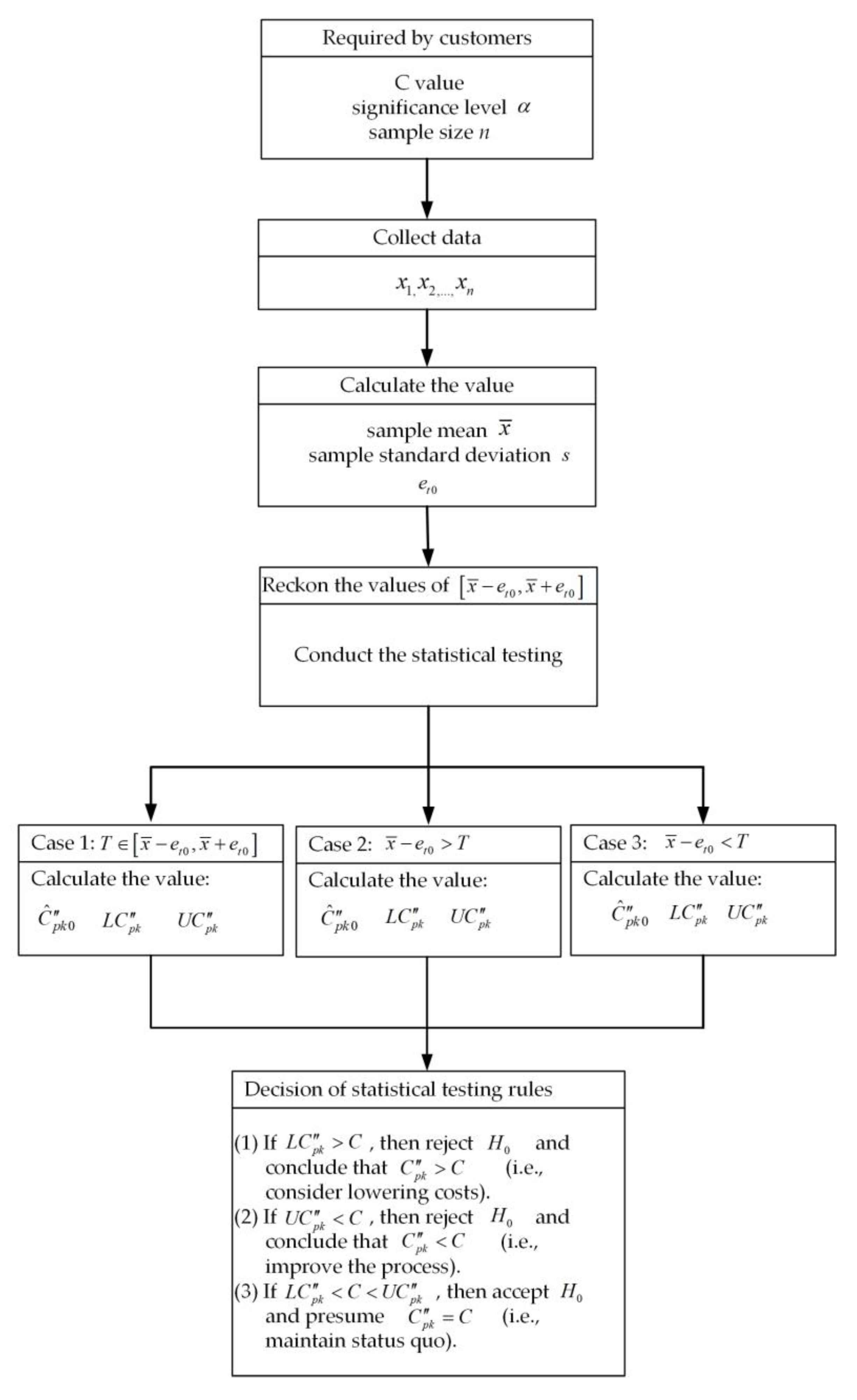
3. Statistical Hypothesis Testing

As described in the previous section, the $100\left(1-\alpha \right)\%$ confidence interval of the asymmetric tolerance index $C_{pk}^{″}$ is represented by the following specification limits:

$$L{C}_{pk}^{″}=\{\begin{array}{l}{\hat{C}}_{pk0}^{″}\times \sqrt{\frac{{\chi }_{\alpha /4;n-1}^2}{n-1}}, T\in \left[\overline{x}-e_{t0}, \overline{x}+e_{t0}\right]\\ \left({\hat{C}}_{pk0}^{″}-\frac{d_l{t}_{\alpha /4;n-1}}{3\sqrt{n}}\right)\times \sqrt{\frac{{\chi }_{\alpha /4;n-1}^2}{n-1}}, \overline{x}+e_{t0}<T\\ \left({\hat{C}}_{pk0}^{″}-\frac{d_u{t}_{\alpha /4;n-1}}{3\sqrt{n}}\right)\times \sqrt{\frac{{\chi }_{\alpha /4;n-1}^2}{n-1}}, \overline{x}-e_{t0}>T\end{array},$$

(30)

$$U{C}_{pk}^{″}=\{\begin{array}{l}{\hat{C}}_{pk0}^{″}\times \sqrt{\frac{{\chi }_{1-\alpha /4;n-1}^2}{n-1}}, T\in \left[\overline{x}-e_{t0}, \overline{x}+e_{t0}\right]\\ \left({\hat{C}}_{pk0}^{″}+\frac{d_l{t}_{\alpha /4;n-1}}{3\sqrt{n}}\right)\times \sqrt{\frac{{\chi }_{1-\alpha /4;n-1}^2}{n-1}}, \overline{x}+e_{t0}<T\\ \left({\hat{C}}_{pk0}^{″}+\frac{d_u{t}_{\alpha /4;n-1}}{3\sqrt{n}}\right)\times \sqrt{\frac{{\chi }_{1-\alpha /4;n-1}^2}{n-1}}, \overline{x}-e_{t0}>T\end{array},$$

(31)

where

$${\hat{C}}_{pk0}^{″}=\{\begin{array}{l}\frac{d}{3s}, T\in \left[\overline{x}-e_{t0}, \overline{x}+e_{t0}\right]\\ \frac{d+d_l\times \left(\overline{x}-T\right)}{3s}, \overline{x}+e_{t0}<T\\ \frac{d-d_u\times \left(\overline{x}-T\right)}{3s}, \overline{x}-e_{t0}>T\end{array}.$$

(32)

Lo et al. [21] defined the following levels for process capability requirements:

(1)

Process capability is considered “inadequate” when $C_{pk}^{″}$ $<$ 1.00.

(2)

Process capability is considered “capable” when 1.00 $\le$ $C_{pk}^{″}$ $<$ 1.33

(3)

Process capability is considered “satisfactory” when 1.33 $\le$ $C_{pk}^{″}$ $<$ 1.5

(4)

Process capability is considered “excellent” when 1.50 $\le$ $C_{pk}^{″}$ $<$ 2.00

(5)

Process capability is considered “superb” when 2.00 $\le$ $C_{pk}^{″}$

To determine whether asymmetric tolerances index $C_{pk}^{″}$ is equal to $c$, we adopt null hypothesis $H_0$:$C_{pk}^{″}$ $=$ $C$ against alternative hypothesis $H_1$:$C_{pk}^{″}$ $\ne$ $C$.

Based on Equations (26) and (27) and with significance level $\alpha$, we construct the following three statistical testing rules:

(1)

If $L{C}_{pk}^{″}$ $>$ $C$, then reject $H_0$ and conclude that $C_{pk}^{″}$ $>$ $C$ (i.e., consider lowering costs).

(2)

If $U{C}_{pk}^{″}$ $<$ $C$, then reject $H_0$ and conclude that $C_{pk}^{″}$ $<$ $C$ (i.e., improve the process).

(3)

If $L{C}_{pk}^{″}$ $<$ $C$ $<$ $U{C}_{pk}^{″}$, then accept $H_0$ and presume $C_{pk}^{″}$ $=$ $C$ (i.e., maintain status quo).

Next, to help the industry successfully apply the proposed assessment model, we established the following procedure:

Step 1: Based on the capability level required by customers, determine the C value, significance level $\alpha$, and sample size n.

Step 2: Figure out the mean and variance of the sample, and $e_{t0}$ based on sample data as follows:

$$\overline{x}=\frac{1}{n}{\displaystyle \sum _{i=1}^n{x}_i},$$

$$s=\sqrt{\frac{1}{n}{\displaystyle \sum _{i=1}^n{\left(x_i-\overline{x}\right)}^2}},$$

$$e_{t0}=t_{\alpha /4;n-1}\times \left(\frac{s}{\sqrt{n}}\right).$$

Step 3: Reckon the values of $\left[\overline{x}-e_{t0},\overline{x}+e_{t0}\right]$ and conduct statistical testing for three cases as follows:

Case 1: T $\in$ $\left[\overline{x}-e_{t0},\overline{x}+e_{t0}\right]$

Figure out ${\hat{C}}_{pk0}^{″}$, $L{C}_{pk}^{″}$, and $U{C}_{pk}^{″}$ as follows:

$${\hat{C}}_{pk0}^{″}=3\frac{1}{{\widehat{\gamma }}_0},$$

$$L{C}_{pk}^{″}={\hat{C}}_{pk0}^{″}\times \sqrt{\frac{{\chi }_{\alpha /4;n-1}^2}{n-1}},$$

$$U{C}_{pk}^{″}={\hat{C}}_{pk0}^{″}\times \sqrt{\frac{{\chi }_{1-\alpha /4;n-1}^2}{n-1}}.$$

Case 2: $\overline{x}-e_{t0}$ $>$ T

Calculate ${\hat{C}}_{pk0}^{″}$, $L{C}_{pk}^{″}$, and $U{C}_{pk}^{″}$ as follows:

$${\hat{C}}_{pk0}^{″}=\frac{d-d_u\left(\overline{x}-T\right)}{3s},$$

$$L{C}_{pk}^{″}=\left({\hat{C}}_{pk0}^{″}-\frac{d_u{t}_{\alpha /4;n-1}}{3\sqrt{n}}\right)\times \sqrt{\frac{{\chi }_{\alpha /4;n-1}^2}{n-1}},$$

$$U{C}_{pk}^{″}=\left({\hat{C}}_{pk0}^{″}+\frac{d_u{t}_{\alpha /4;n-1}}{3\sqrt{n}}\right)\times \sqrt{\frac{{\chi }_{1-\alpha /4;n-1}^2}{n-1}}.$$

Case 3: $\overline{x}+e_{t0}$ $<$ T

Calculate ${\hat{C}}_{pk0}^{″}$, $L{C}_{pk}^{″}$, and $U{C}_{pk}^{″}$ as follows:

$${\hat{C}}_{pk0}^{″}=\frac{d+d_l\left(\overline{x}-T\right)}{3s},$$

$$L{C}_{pk}^{″}=\left({\hat{C}}_{pk0}^{″}-\frac{d_l{t}_{\alpha /4;n-1}}{3\sqrt{n}}\right)\times \sqrt{\frac{{\chi }_{\alpha /4;n-1}^2}{n-1}},$$

$$U{C}_{pk}^{″}=\left({\hat{C}}_{pk0}^{″}+\frac{d_l{t}_{\alpha /4;n-1}}{3\sqrt{n}}\right)\times \sqrt{\frac{{\chi }_{1-\alpha /4;n-1}^2}{n-1}}.$$

Step 4: According to the values of $L{C}_{pk}^{″}$ and $U{C}_{pk}^{″}$ in each of the three cases, conduct statistical verification using the statistical testing rules.

Besides the above steps, we also have made a flowchart, as shown in Figure 2, for making clear the methodology proposed in this section as follows:

4. An Illustrative Example

The quality characteristics of many machinery products have asymmetric tolerances [1,2,3]. Say, for instance, that the asymmetric tolerance of a quality characteristic for a machine part is $\left(LSL,T,USL\right)$ $=$ (4.03, 4.05, 4.10). This gives us the following parameters:

upper tolerance $D_u$ $=$ $USL-T$ $=$ 4.10 $-$ 4.05 $=$ 0.05,

lower tolerance $D_l$ $=$ $T-LSL$ $=$ 4.05 $-$ 4.03 $=$ 0.02,

$$d=Min\left\{D_u,D_l\right\}=0.02,$$

$$d_u=\frac{d}{D_u}=0.4,$$

$$d_l=\frac{d}{D_l}=1.0.$$

According to the evaluation procedure provided in Section 3, we perform the following steps:

Step 1: Based on the capability level required by customers, we calculate the following:

Required capability: C $=$ 1.0,

Significance level: $\alpha$ = 0.05,

Sample size: n $=$ 36,

Null hypothesis: $H_0$:$C_{pk}^{″}$ $=$ 1.0,

Alternative hypothesis: $H_1$:$C_{pk}^{″}$ $\ne$ 1.0.

Step 2: We then calculate the value of sample mean $\overline{x}$, sample standard deviation $s$, and $e_{t0}$ with sample size n $=$ 36, as follows:

$$\overline{x}=\frac{1}{36}{\displaystyle \sum _{i=1}^{36}{x}_i}=4.07,$$

$$s=\sqrt{\frac{1}{36}{\displaystyle \sum _{i=1}^{36}{\left(x_i-\overline{x}\right)}^2}}=0.005,$$

$$e_{t0}=t_{\alpha /4;n-1}\times \left(\frac{s}{\sqrt{n}}\right)=t_{0.025;35}\times \left(\frac{0.005}{\sqrt{36}}\right)=\left(\frac{0.005}{\sqrt{36}}\right)=0.0017.$$

Obviously, the estimated error item is less than or equal to $0.0017$ when n $=$ 36 $\left(\left|\overline{x}-\mu \right|\le 0.0017\right)$. If $e_{t0}$ is required to be smaller than 0.0017, the sample size of n needs to be larger. The value of n can be calculated by the inequality as shown below:

$$n\ge {\left(\frac{s}{e_{t0}}{t}_{\alpha /4;n-1}\right)}^2.$$

Step 3: Next, we calculate the values of $\left[\overline{x}-e_{t0},\overline{x}+e_{t0}\right]$ as follows:

$$\left[\overline{x}-e_{t0},\overline{x}+e_{t0}\right]=\left[4.07-0.0017,4.07+0.0017\right]=\left[4.0683,4.0717\right].$$

Since $\overline{x}-e_{t0}$ $=$4.0683 $>$ 4.05, we calculate the values of ${\hat{C}}_{pk0}^{″}$, $L{C}_{pk}^{″}$, and $U{C}_{pk}^{″}$ for case (2) as follows:

$${\hat{C}}_{pk0}^{″}=\frac{d-d_u\left(\overline{x}-T\right)}{3s}=\frac{0.02-0.4\times \left(4.07-4.05\right)}{3\times 0.005}=0.8,$$

$$L{C}_{pk}^{″}=\left({\hat{C}}_{pk0}^{″}-\frac{d_u\times t_{0.025;35}}{3\sqrt{n}}\right)\times \sqrt{\frac{{\chi }_{0.025;35}^2}{n-1}}=\left(0.8-\frac{0.4\times 2.03}{3\sqrt{36}}\right)\times \sqrt{\frac{20.569}{35}}=0.579,$$

$$U{C}_{pk}^{″}=\left({\hat{C}}_{pk0}^{″}+\frac{d_u{t}_{\alpha /4;n-1}}{3\sqrt{n}}\right)\times \sqrt{\frac{{\chi }_{1-\alpha /4;n-1}^2}{n-1}}=\left(0.8+\frac{0.4\times 2.03}{3\sqrt{36}}\right)\times \sqrt{\frac{53.203}{35}}=0.919.$$

Step 4: We use $L{C}_{pk}^{″}$ $=$ 0.579 and $U{C}_{pk}^{″}$ $=$ 0.919 to conduct statistical verification as follows:

Since $U{C}_{pk}^{″}$ $=$ 0.919 $<$ $C$ $=$ 1.0, we reject $H_0$ and conclude that the process is inadequate ($C_{pk}^{″}$ $<$ 1.0) and therefore in need of improvement.

5. Conclusions and Further Research

The quality characteristics of many important machine tool parts have asymmetric tolerances. Asymmetric tolerance index $C_{pk}^{″}$ is a function of $\mu$ and $\sigma$, which means it simultaneously depends on $\mu$ and $\sigma$. Unfortunately, it is difficult to derive the confidence interval of index $C_{pk}^{″}$. This study therefore adopts Boole’s inequality and DeMorgan’s theorem to discover the combined confidence region of $\left(\mu ,\sigma \right)$. Next, using index $C_{pk}^{″}$ as the objective function and the $100\left(1-\alpha \right)\%$ confidence region of $\left(\mu ,\sigma \right)$ as the feasible region, this study applies mathematical programming for the $100\left(1-\alpha \right)\%$ confidence interval of index $C_{pk}^{″}$ and also employs it for the statistical hypothesis test to see if the process capabilities of QCs with asymmetric tolerances can meet the required quality levels. Last, this study provides an illustration to demonstrate the feasibility of the proposed method. The advantages of this model proposed in this study are able to apply to evaluate the process quality of the asymmetric tolerance and symmetrical tolerance products at the same time and reduce the misjudgment risk of sampling error owing to testing through the confidence interval.

Since this study focuses on the normal distribution of a single process only, the statistical tests of multivariate asymmetric tolerance indicators can be included for future study. Meanwhile, the normal process distribution is a common research hypothesis, so this article focuses on parameters tests. However, the non-normal distribution of the process is explored in many research [22,23,24,25]. Therefore, nonparametric tests can be views as the important topic for further study.

References

1. Lin, K.P.; Yu, C.M.; Chen, K.S. Production data analysis system using novel process capability indices-based circular economy. Ind. Manag. Data Syst. 2019, 119, 1655–1668. [Google Scholar] [CrossRef]
2. Chien, C.F.; Hong, T.Y.; Guo, H.Z. An empirical study for smart production for TFT-LCD to empower Industry 3.5. J. Chin. Inst. Eng. 2017, 40, 552–561. [Google Scholar] [CrossRef]
3. Chen, K.S.; Wang, C.H.; Tan, K.H. Developing a fuzzy green supplier selection model using Six Sigma quality indices. Int. J. Prod. Econ. 2019, 212, 1–7. [Google Scholar] [CrossRef]
4. Prahalad, C.K.; Hamel, G. The Core Competence of the Corporation. Harv. Bus. Rev. 1990, 68, 79–91. [Google Scholar]
5. Grossman, G.M.; Helpman, E. Integration versus outsourcing in industry equilibrium. Q. J. Econ. 2002, 117, 85–120. [Google Scholar] [CrossRef]
6. Chen, K.S. Incapability index with asymmetric tolerances. Stat. Sin. 1998, 8, 253–262. [Google Scholar]
7. Pearn, W.L.; Lin, P.C.; Chen, K.S. The C′′pk index for asymmetric tolerances: Implications and inference. Metrika 2004, 60, 119–136. [Google Scholar] [CrossRef]
8. Shu, M.H.; Chen, K.S. Estimating process capability indices based on subsamples for asymmetric tolerances. Commun. Stat. Theory Methods 2005, 34, 485–505. [Google Scholar] [CrossRef]
9. Chuang, C.J.; Wu, C.W. Determining optimal process mean and quality improvement in a profit-maximization supply chain model. Qual. Technol. Quant. Manag. 2019, 16, 154–169. [Google Scholar] [CrossRef]
10. Shafer, S.M.; Moeller, S.B. The effects of Six Sigma on corporate performance: An empirical investigation. J. Oper. Manag. 2012, 30, 521–532. [Google Scholar] [CrossRef]
11. Anderson, N.C.; Kovach, J.V. Reducing welding defects in turnaround projects: A lean six sigma case study. Qual. Eng. 2014, 26, 168–181. [Google Scholar] [CrossRef]
12. Yang, C.M.; Chen, K.S.; Hsu, T.H.; Hsu, C.H. Supplier selection and performance evaluation for high voltage power film capacitors in fuzzy environment. Appl. Sci. 2019, 9, 5253. [Google Scholar] [CrossRef] [Green Version]
13. Abbasi Ganji, Z.; Sadeghpour Gildeh, B. A new multivariate process capability index. Total Qual. Manag. Bus. Excell. 2017, 30, 525–536. [Google Scholar] [CrossRef]
14. Nikzad, E.; Amiri, A.; Amirkhani, F. Estimating total and specific process capability indices in three-stage processes with measurement errors. J. Stat. Comput. Simul. 2018, 88, 3033–3064. [Google Scholar] [CrossRef]
15. Besseris, G.J. Evaluation of robust scale estimators for modified Weibull process capability indices and their bootstrap confidence intervals. Comput. Ind. Eng. 2019, 128, 135–149. [Google Scholar] [CrossRef]
16. de-Felipe, D.; Benedito, E. Monitoring high complex production processes using process capability indices. Int. J. Adv. Manuf. Technol. 2017, 93, 1257–1267. [Google Scholar] [CrossRef] [Green Version]
17. Kane, V.E. Process capability indices. J. Qual. Technol. 1986, 18, 41–52. [Google Scholar] [CrossRef]
18. Boyles, R.A. Process capability with asymmetric tolerances. Commun. Stat. Simul. Comput. 1994, 23, 615–643. [Google Scholar] [CrossRef]
19. Pearn, W.L.; Chen, K.S. New generalization of the process capability index Cpk. J. Appl. Stat. 1998, 25, 801–810. [Google Scholar] [CrossRef]
20. Chen, K.S.; Huang, C.F.; Chang, T.C. A mathematical programming model for constructing the confidence interval of process capability index Cpm in evaluating process performance: An example of five-way pipe. J. Chin. Inst. Eng. 2017, 40, 126–133. [Google Scholar] [CrossRef]
21. Lo, W.; Yang, C.M.; Lai, K.K.; Li, S.Y.; Chen, C.H. Developing a Novel Fuzzy Evaluation Model by One-Sided Specification Capability Indices. Mathematics 2021, 9, 1076. [Google Scholar] [CrossRef]
22. Pearn, W.L.; Chen, K.S. Estimating process capability indices for non-normal pearsonian populations. Qual. Reliab. Eng. Int. 1995, 11, 386–388. [Google Scholar] [CrossRef]
23. Liao, S.J.; Chen, K.S.; Li, R.K. Capability evaluation for processes of the larger-the-better type for non-normal populations. Adv. Appl. Stat. 2002, 2, 189–198. [Google Scholar]
24. Erfanian, M.; Sadeghpour Gildeh, B. A new capability index for non-normal distributions based on linex loss function. Qual. Eng. 2021, 33, 76–84. [Google Scholar] [CrossRef]
25. Farokhnia, M.; Niaki, S.T.A. Principal component analysis-based control charts using support vector machines for multivariate non-normal distributions. Commun. Stat. Simul. Comput. 2020, 49, 1815–1838. [Google Scholar] [CrossRef]
Figure 1. Conceptual framework of the Introduction section.
Applsci 11 06249 g001
Figure 2. Flowchart of statistical hypothesis testing.
Applsci 11 06249 g002
Publisher’s Note: MDPI stays neutral with regard to jurisdictional claims in published maps and institutional affiliations.