Article

Multiparametric Analysis of a Gravity Retaining Wall

Faculty of Civil Engineering, Transportation Engineering and Architecture, University of Maribor, Smetanova Ulica 17, 2000 Maribor, Slovenia
*
Author to whom correspondence should be addressed.
Appl. Sci. 2021, 11(13), 6233; https://doi.org/10.3390/app11136233
Submission received: 21 May 2021 / Revised: 29 June 2021 / Accepted: 1 July 2021 / Published: 5 July 2021
(This article belongs to the Special Issue New Frontiers in Buildings and Construction)

Abstract

:
The design of a gravity retaining wall should be simple to construct, quick to build and the best economic solution to a problem. This can be achieved by using advanced optimization methods. Since geotechnical engineers are not always able to determine the exact soil properties and other project data, an optimal design of a gravity retaining wall should also be determined for a wide range of input parameters. Therefore, a multiparametric analysis of an optimal designed gravity retaining wall was carried out. Optimum designs of gravity retaining walls were obtained for 567 combinations of different design parameters. Diagrams were developed to help engineers determine the optimum section of the wall, based on construction costs. An exhaustive search was carried out within the available parameters (project data). The parameters were ranked according to which had the most influence on the optimum cost of the gravity retaining wall and the utilization of multiple constraints. The most important parameter for the optimal cost of a gravity retaining wall is the height of the retained ground, followed by the shear angle of the soil, the soil–wall interaction coefficient, the slope angle and the variable surcharge load. The shear angle of the soil is most relevant to the bearing capacity and eccentricity condition, while the soil–wall interaction coefficient is most relevant to the sliding condition. Since European countries apply different load, material and resistance safety factors, the optimization model was developed in a general form, where different design approaches and unit prices could be applied. The case study provides an improved optimization model for selecting the optimal design of gravity walls, for engineers.

1. Introduction

Highways and local road networks are the most important land infrastructure in the European Union. Retaining walls make up a significant proportion of the fixed assets of the highways and local road networks and are vital elements. Their failure can have serious economic consequences. According to Eurocode 7 [1], a retaining wall is defined as an earth retaining structure supporting at least 2 m of ground, i.e., the soil level in front of the wall is ≥2 m lower than the soil level behind the wall. Such structures fall into geotechnical category 2 or 3 of Eurocode 7 and must be designed by a suitably qualified person. The report COST Action 345 [2] collects information on the number and type of retaining structures in European countries and highlights the importance of the annual cost of maintaining, repairing, renewing and replacing these structures. In the United Kingdom, the average length of retaining walls per km of whole road systems is about 11.1 m/km. The majority of retaining walls in the United Kingdom are gravity retaining walls, about 85%. The other 15% are reinforced concrete retaining walls. Ninety-five percent of all retaining walls measure less than 6 m in height. The average replacement cost per m for a retaining wall in the United Kingdom, Spain and Denmark is estimated at 1550, 560 and 4390 EUR/m respectively.
In geotechnical engineering, gravity retaining walls are used to secure slopes that do not have long-term stability for providing lateral soil load resistance. This paper deals with masonry retaining walls consisting of stones with bedded concrete of low compressive strength. In designing gravity retaining walls, stability conditions such as sliding, overturning, eccentricity and bearing capacity are evaluated using selected wall dimensions. If the initially selected dimensions do not satisfy the stability conditions, new dimensions are selected and reevaluated until the stability conditions are satisfied. Even if the conditions are met, it is not certain that the determined wall dimensions will ultimately result in the most economical wall design. Optimization is required to satisfy all conditions and obtain the lowest possible cost. Calculations used to determine the external and internal stability of masonry walls should be carried out according to the Eurocode 7 standard. The final design of a gravity retaining wall should be simple to construct, quick to build and the best economic solution to the problem.
In the recent past, many heuristic optimization algorithms have been used in the field of civil engineering. However, not many of them have been applied in the field of geotechnical engineering. Concrete retaining walls have been optimized to the optimal design using eleven population-based metaheuristic algorithms; all the algorithms used quickly converged to high-quality optimal designs [3,4,5,6]. Optimizations for reinforced concrete retaining walls, in terms of cost and weight, have been made by several authors [7,8,9,10,11]. Gravity retaining walls of stone masonry or unreinforced concrete have also been investigated [12,13]. Stability analyses of gravity retaining walls, for different wall-back types, have been performed but not optimized [14]. In a detailed comparative study, different optimization methods were shown for geotechnical problems and their effects on the variation of studied parameters [15]. Multiparametric optimizations on different civil engineering structures have been studied by several authors [16,17,18]. Kravanja et al. [19] discussed a comparative study of an optimal design for composite steel–concrete floor structures based on the multiparametric mixed-integer nonlinear programming (MINLP) approach. The multiparametric optimization approach has also been applied in the field of geotechnical engineering, e.g., in the design of piled embankments with basal reinforcement [20,21], conventional [22,23] and geothermal energy piles [24,25], reinforced pad and strip foundations [26,27] and geosynthetic-reinforced soil bridge abutments [28]. Several studies have evaluated the sustainability of the most common earth retaining walls such as gabion walls, crib walls, masonry walls, mechanically stabilized earth walls and reinforced concrete walls. They indicated that masonry walls and mechanically stabilized earth walls are the most sustainable alternatives, while reinforced concrete walls have the lowest sustainability performance [29,30,31]. However, it seems that multiparametric cost optimizations of gravity retaining walls, according to the Eurocode 7 standard, have not yet been investigated in research papers.
In order to reduce the construction cost of gravity retaining walls, three main parts are presented in this paper. In the first part, the mathematical problem of a gravity retaining wall is described and includes all the design conditions and the cost objective function, from which it is possible to find the minimum construction cost of the wall by applying the real coded genetic algorithm [32]. In the second part, a parametric analysis of a gravity retaining wall was carried out. The optimum design of gravity retaining walls was obtained for 567 combinations of different design parameters. Diagrams were developed to help engineers determine the optimum section of the wall. In the last part, an exhaustive search was carried out within the available parameters (project data). They were then ranked according to the parameters that have the most influence on the optimum cost of a gravity retaining wall and the utilization of multiple constraints.

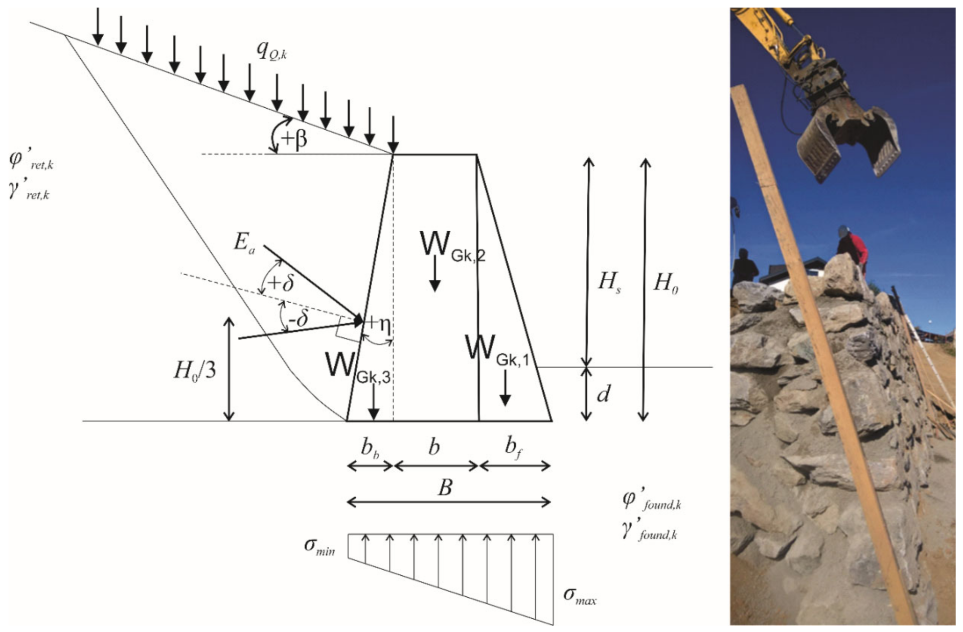
2. Mathematical Model of a Gravity Retaining Wall

In designing gravity retaining walls, an engineer must start from their dimensions. This is not a trivial task, however, because soil conditions, terrain configuration and other conditions are specific to each site. Even more difficult is the selection of appropriate dimensions that meet all geotechnical conditions with a minimal cost. Therefore, sections of the gravity retaining wall need to be iteratively modified and geotechnical conditions need to be rechecked. This iterative process can be performed by optimization algorithms capable of testing a large number of different wall sections in a short period of time. In order to apply optimization algorithms, a mathematical representation of the gravity retaining wall problem must be defined. This is called an optimization model. Table 1 shows such an optimization model, where the cost objective function, geotechnical constraints and design constraints of a gravity retaining wall are defined. It should be noted that this study provides an improved optimization model that takes into account not only soil mechanics conditions, but also good design-practice conditions. The optimization model includes input data and variables. The input data represent the given project requirements and the site conditions along with economic data. The following geometric variables are used in optimization models (see Figure 1): width of the front wall section bf (m), width of the middle wall section b (m), width of the rear wall section bb (m), depth of the embedded gravity wall d (m) and the retaining wall construction cost defined as COST (EUR/m).
The objective function COST (see Equation (1)) includes the construction cost of the gravity retaining wall. This includes the material cost, soil excavation, fill material with compaction and the drainage system. Therefore, the optimal solution represents the minimum cost of a gravity retaining wall that satisfies all the design and stability constraints. The optimization consists of 6 conditions that must be met. The first condition states that the horizontal force acting on the retaining wall cannot exceed the sum of the resistances below the wall (see Equation (2)). It is defined by Equations (2a)–(2ae) and must be satisfied. The eccentricity of the action from the center of the wall eB (m) is bounded by the maximum allowable eccentricity emax. This limit is represented by the second condition (see Equation (3)) and is further defined by Equations (3a)–(3m). Condition 3 (see Equation (4)) limits the bearing capacity. The applied vertical load on the foundation plane Vd must be less than the bearing capacity of the foundation soil Rd. The equations used to calculate this condition (see Equations (4a)–(4l)) consider the wall to be a strip foundation. Condition 4 (see Equation (5)) is for preventing overturning failure. This is only relevant for gravity retaining walls constructed on strong foundations. The dimensions of the gravity retaining wall are constrained by the limits given in Equations (6)–(6b) and the discrete alternatives in Table 1. The earth pressure coefficients are determined by a numerical procedure. Since the back face of the wall may be inclined at an angle η to the vertical, the effective earth pressures acting on the wall are inclined. Therefore, the earth pressure coefficients are determined by a numerical procedure defined in the Eurocode 7 standard, rather than by simple Rankine earth pressure coefficients that ignore friction along the wall. However, the Eurocode 7 standard does not cover the specific requirements of seismic design. Therefore, several researchers have proposed models to estimate the magnitude and variation of seismic earth pressures acting on the backs of the gravity walls [33,34,35].
The real coded genetic algorithm (RCGA) was applied to test a large number of different wall sections and to select the design of a gravity retaining wall with minimum construction costs [32]. The maximum number of iterations and the population size for the genetic algorithm to perform were set as 200 and 300, respectively. The number of individuals guaranteed to survive to the next generation was fixed at 10. In this optimization, rank scaling was used, which scales the raw scores based on each individual’s rank instead of their score. In this way, the effect of large scattering in the raw scores was removed. RCGA stops when the average relative change in the best fitness function value over stall generations (max assigned stall generation is 50) is less than or equal to the function tolerance (1 × 10⁻⁸). The time it took the CPU to find a single optimal solution was 6.95 s. The computer used for the optimization was an Intel Pentium i7 with a 2.2 GHz processor. Furthermore, when the population size was increased from 300 to 3000, the CPU time increased by 5.67 s. The results of the optimization process are presented in the next section, where the optimal designs for different project data are determined.

3. Parametric Analysis of a Gravity Retaining Wall

The optimization model presented above was developed in a general form so that an optimal design for a gravity retaining wall can be obtained for any project data (e.g., soil properties, terrain configuration, loads). A series of optimizations of a gravity retaining wall were performed for a combination of different parameters, i.e., different values of retaining wall heights HS, soil shear angle φk, soil–wall interaction coefficient k, slope angle β and surcharge load qQk. The soil–wall interaction coefficient k (δ/φ) was used to determine the angle of interface friction between the soil and the wall (δ) based on the soil friction angle (φ). Input data, variables and a cost objective function subjected to (in)equality geotechnical and design constraints were included in the model. The optimal cost and dimensions of the gravity retaining wall were determined for each optimization. An RCGA was used to solve the optimization problems. A parametric optimization was performed for all 567 combinations of the following different design parameters:
  • Seven different wall heights Hs:
2, 2.5, 3, 3.5, 4, 4.5 and 5 m;
2.
Three different shear angles of soil φk:
30, 35 and 40°;
3.
Three different soil–wall interaction coefficients k:
1/2, 2/3 and 1;
4.
Three different slope angles β:
0, 10 and 20°;
5.
Three different surcharge loads qQk:
0, 2 and 4 kPa.
The input data used in the optimization model are shown in Table 2 and remain constant in the multiparametric analysis. Note that in the multiparametric analysis, the shear angle of the retained ground and the shear angle of the foundation soil are assumed to be equal (φret,k = φfound,k = φk). The same assumption was used for the soil–wall interaction coefficient (kret = kfound = k). The subscript “ret” denotes the properties of retaining soil, while the subscript “found” denotes the properties of the foundation soil. The partial safety factors correspond to design approach 1 (combination 2) defined in Eurocode standard 7 [1].
Figure 2 shows the optimal results for a gravity retaining wall with a soil–wall interaction coefficient k = 2/3, slope angle β = 0° and variable surcharge load qQk = 0 kPa. With the help of these diagrams, it is possible to determine the optimal wall dimension (bf, b, B and d) and which geotechnical constraints have the highest degree of utilization. Note that nonsmooth graphs of optimal wall dimensions were obtained while the wall dimensions were defined as discrete variables. The optimum construction costs and weight of the gravity retaining wall can also be determined. It can be clearly seen that for weak soil (φk = 30°), the sliding failure and the bearing capacity failure are decisive, while for strong soil (φk = 40°), the eccentricity condition determines the optimal design. In all 567 combinations, the optimal width of the rear wall section bb was found to be 0 m. A retaining wall with a height Hs = 4 m, supporting the ground with a shear angle φk = 35°, has optimal dimensions of bf = 1.3 m, B = 1.8 m, b = 0.5 m and d = 0.6 m. For the optimal design, the construction cost and weight of the wall are approximately 850 EUR/m and 150 kN/m, respectively. The bearing capacity condition has the highest utilization rate of about 96%. Using the procedure described above, 567 individual optimizations were performed for all 567 combinations of the various defined parameters, yielding 567 different optimal results. These results are shown graphically in the diagrams in Figure 3, Figure 4, Figure 5, Figure 6, Figure 7, Figure 8, Figure 9, Figure 10 and Figure 11. These figures allow the engineer to obtain optimum design parameters of a gravity retaining wall for various project data. For example, a gravity wall with a height Hs = 2.5 m and other project data such as k = 0.5, β = 20°, γ = 18 kN/m3 and qQk = 4 kPa has an optimal design that includes bf = 2.1 m, d = 1.6 m and b = 0.6 m, as shown in Figure 3.

4. Sensitivity Analysis

The optimal design of the gravity retaining wall was determined for different input data. The five main input data are the height of the retained ground (Hs), the variable surcharge load (qQ,k), the slope angle (β), the shear angle of the soil (φk = φret = φfound) and the interaction coefficient between the soil and the retaining wall (k = kret = kfound). The main objective of this multiparametric analysis was to use these main attributes to predict other continuous attributes, such as the optimal cost of the retaining wall (COST), the utilization of the bearing capacity condition (Vd/Rd), the utilization of sliding condition (HEd/HRd) and the utilization of the eccentricity condition (eB/emax). Before applying the predictive model, the dataset was divided into a training dataset (odd indexed samples) and a checking dataset (even indexed samples). The “exhsrch” function included in MATLAB was used to perform an exhaustive search within the available inputs to select the set of inputs that have the greatest impact on the optimal cost of the gravity retaining wall and the utilization of multiple constraints. For the “exhsrch” function, the predictive models were built for each parameter combination and trained for an epoch; the achieved performance was then reported. The leftmost input variable in Figure 12 is the most relevant in terms of output, while it has the lowest root-mean-square error (RMSE). The RMSE is defined as follows:
R M S E = i = 1 n x ^ i x i 2 n
where x ^ i are the predicted values and x i are the values obtained by the optimization procedure (COST, Vd/Rd, HEd/HRd, eB/emax). The prediction models are often subject to the problem of overfitting. However, in this simple prediction model, it can be seen that the training and checking errors are comparable, which means that there is no overfitting. It should be noted that the main objective of this prediction model is to find the inputs that have the greatest impact on the output, not to build the prediction model with minimum training error. It also examines the combination of two inputs that have the greatest influence on the output. The result of the parametric analysis clearly shows that the most important parameter for the optimal cost of a gravity retaining wall is the height of the retained ground, followed by the shear angle of the soil, the interaction coefficient, the slope angle and the variable surcharge load. The shear angle of the soil is most relevant to the bearing capacity and eccentricity condition, while the interaction coefficient is most relevant to the sliding condition. The parametric analysis also shows that the “height of the retained ground” and the “shear angle of the soil” form the optimal combination of two inputs that are most relevant to the optimal cost and bearing capacity condition. However, the combination of “shear angle of soil” and “interaction coefficient” is most relevant for the sliding and eccentricity condition.

5. Conclusions

The optimization was performed 567 times to obtain an optimal design of a gravity retaining wall for different site characteristics and project data. The results of this study will help engineers to determine the wall section in the first iteration that meets the stability requirements and minimum construction costs. During optimization, some of the geotechnical constraints were fully exploited, so this paper also discusses which geotechnical constraints govern the design. Critical geotechnical constraints also depend on the site characteristics and project data. While geotechnical engineers are not always able to determine the exact soil properties, this study is appropriate for determining what effect vague input data have on the cost of a gravity retaining wall. The following conclusions can be drawn based on the multiparametric analysis:
  • The optimal width of the front wall section bf reached the highest values among all dimensions of the wall, while the optimal width of the rear wall section bb was found to be 0 m at all different combinations of parameters.
  • The most important parameter for the optimal cost of the gravity retaining wall is the height of the retained ground, followed by the shear angle of the soil, the soil–wall interaction coefficient, the slope angle and the variable surcharge load.
  • The shear angle of the soil is most relevant to the bearing capacity and eccentricity condition, while the interaction coefficient is most relevant to the sliding condition.
  • Given the unfavorable site characteristics and project data (φk = 30°, k = 0.5, β = 20°, qQk = 0 kPa), doubling the height of the retaining wall (from 2.5 to 5 m) increases the cost from 653.7 to 2510.7 EUR/m, almost four times the cost of a smaller wall.
  • Gravity retaining walls are usually sloped toward the earth mass behind them to counteract the force of gravity acting against them, which is called “setback”. Based on the parametric analysis, the optimum angle of this slope ranges from 7 to 47°, with an average value of about 18° (slope ratio HD/VD = 1:3).
  • The depth of the foundation for a gravity retaining wall depends on the height of the wall. Based on the parametric analysis, the optimum depth of the retaining wall is between 10 and 40% of the height of the wall, with an average value of 20% (one-fifth of its height below ground level).
The article gives recommendations for the optimal design of gravity retaining walls. The usefulness of the developed diagrams is illustrated with examples. While European countries adopt different load, material and resistance factors, the Eurocode 7 standard defines three design approaches. Since the cost of building a gravity retaining wall depends on key parameters such as quantity of materials, unit material prices and labor costs, an economically optimal design may also change as the relative ratios among the key parameters change. The optimal designs of gravity retaining walls in this paper correspond only to design approach 1 (combination 2). Because the optimization model was developed in a general form, other design approaches and unit prices can also be considered, and their influence on the optimal design can be further investigated.

Author Contributions

Conceptualization, P.J.; methodology, P.J.; formal analysis, P.J. and R.V.; writing—original draft preparation, P.J., B.Ž. and R.V. All authors have read and agreed to the published version of the manuscript.

Funding

This research was funded by the Slovenian Research Agency (grant number P2-0268) and the GEOLAB project (grant number 101006512).

Institutional Review Board Statement

Not applicable.

Informed Consent Statement

Not applicable.

Data Availability Statement

The data presented in this study are available upon request from the corresponding author.

Conflicts of Interest

The authors declare no conflict of interest.

References

  1. EN 1997-1. Eurocode 7: Geotechnical Design Part 1, General Rules. 2004. Available online: https://www.ngm2016.com/uploads/2/1/7/9/21790806/eurocode_7_-_geotechnical_designen.1997.1.2004.pdf (accessed on 20 May 2021).
  2. Brady, K.C.; O’Reilly, M.; Bevc, L.; Žnidarič, A.; O’Brien, E.; Jordan, R. COST 345. Working Group 1. Report on the Current Stock of Highway Structures in European Countries, the Cost of Their Replacement and the Annual Costs of Maintaining, Repairing and Renewing Them. Available online: http://cost345.zag.si/Reports/COST_345_WG1.pdf (accessed on 25 May 2021).
  3. Kaveh, A.; Hamedani, K.B.; Bakhshpoori, T. Optimal Design of Reinforced Concrete Cantilever Retaining Walls Utilizing Eleven Meta-Heuristic Algorithms: A Comparative Study. Period. Polytech. Civ. Eng. 2020, 64, 156–168. [Google Scholar] [CrossRef]
  4. Kaveh, A.; Soleimani, N. CBO and DPSO for optimum design of reinforced concrete cantilever retaining walls. Asian J. Civ. Eng. 2015, 16, 751–774. [Google Scholar]
  5. Kaveh, A.; Behnam, A.F. Charged System Search Algorithm for the Optimum Cost Design of Reinforced Concrete Cantilever Retaining Walls. Arab. J. Sci. Eng. 2013, 38, 563–570. [Google Scholar] [CrossRef]
  6. Konstandakopoulou, F.; Tsimirika, M.; Pnevmatikos, N.; Hatzigeorgiou, G.D. Optimization of Reinforced Concrete Retaining Walls Designed According to European Provisions. Infrastructures 2020, 5, 46. [Google Scholar] [CrossRef]
  7. Sarıbaş, A.; Erbatur, F. Optimization and Sensitivity of Retaining Structures. J. Geotech. Eng. 1996, 122, 649–656. [Google Scholar] [CrossRef]
  8. Khajehzadeh, M.; Taha, M.R.; El-Shafie, A.; Eslami, M. Economic design of retaining wall using particle swarm optimization with passive congregation. Aust. J. Basic Appl. Sci. 2010, 4, 5500–5507. [Google Scholar]
  9. Camp, C.V.; Akin, A. Design of Retaining Walls Using Big Bang–Big Crunch Optimization. J. Struct. Eng. 2012, 138, 438–448. [Google Scholar] [CrossRef]
  10. Moayyeri, N.; Gharehbaghi, S.; Plevris, V. Cost-Based Optimum Design of Reinforced Concrete Retaining Walls Considering Different Methods of Bearing Capacity Computation. Mathematics 2019, 7, 1232. [Google Scholar] [CrossRef] [Green Version]
  11. Kumar, V.N.; Suribabu, C.R. Optimal design of cantilever retaining wall using differential evolution algorithm. Iran Univ. Sci. Technol. 2017, 7, 433–449. [Google Scholar]
  12. Talatahari, S.; Sheikholeslami, R.; Shadfaran, M.; Pourbaba, M. Optimum Design of Gravity Retaining Walls Using Charged System Search Algorithm. Math. Probl. Eng. 2012, 2012, 1–10. [Google Scholar] [CrossRef]
  13. Sadoglu, E. Design optimization for symmetrical gravity retaining walls. Acta Geotech. Slov. 2014, 11, 71–79. [Google Scholar]
  14. Zhuang, J.; Chen, J. Stability Analysis of Gravity Retaining Walls with Different Wall-back Types under Equal Section Area. In IOP Conference Series: Earth and Environmental Science, Proceedings of the 2020 International Conference on Innovative Solutions in Hydropower and Environmental and Civil Engineering, Beijing, China, 11–13 December 2020; IOP Publishing: Bristol, UK, 2021; Volume 668. [Google Scholar]
  15. Nama, S.; Saha, A.K.; Ghosh, S. Parameters Optimization of Geotechnical Problem Using Different Optimization Algorithm. Geotech. Geol. Eng. 2015, 33, 1235–1253. [Google Scholar] [CrossRef]
  16. Qiong, G.; Meng-Gang, Y.; Jian-Dong, Q. A multi-parameter optimization technique for prestressed concrete cable-stayed bridges considering prestress in girder. Struct. Eng. Mech. 2017, 64, 567–577. [Google Scholar] [CrossRef]
  17. Rumpf, M.; Grohmann, M.; Eisenbach, P.; Hauser, S. Structural Surface—Multi parameter structural optimization of a thin high performance concrete object. In Proceedings of the International Association for Shell and Spatial Structures (IASS), Amsterdam, The Netherlands, 17–20 August 2015. [Google Scholar]
  18. Jelusic, P.; Kravanja, S. Optimal design of timber-concrete composite floors based on the multi-parametric MINLP optimization. Compos. Struct. 2017, 179, 285–293. [Google Scholar] [CrossRef]
  19. Kravanja, S.; Žula, T.; Klanšek, U. Multi-parametric MINLP optimization study of a composite I beam floor system. Eng. Struct. 2017, 130, 316–335. [Google Scholar] [CrossRef]
  20. Chen, C.; Mao, F.; Zhang, G.; Huang, J.; Zornberg, J.; Liang, X.; Chen, J. Settlement-Based Cost Optimization of Geogrid-Reinforced Pile-Supported Foundation. Geosynth. Int. 2021, 1–39, online ahead of print. [Google Scholar] [CrossRef]
  21. Jelušič, P.; Žlender, B. Optimal design of piled embankments with basal reinforcement. Geosynth. Int. 2018, 25, 150–163. [Google Scholar] [CrossRef]
  22. Nguyen, D.D.C.; Kim, D.-S.; Jo, S.-B. Parametric study for optimal design of large piled raft foundations on sand. Comput. Geotech. 2014, 55, 14–26. [Google Scholar] [CrossRef]
  23. Leung, Y.F.; Klar, A.; Soga, K. Theoretical Study on Pile Length Optimization of Pile Groups and Piled Rafts. J. Geotech. Geoenviron. Eng. 2010, 136, 319–330. [Google Scholar] [CrossRef]
  24. Jelušič, P.; Žlender, B. Determining optimal designs for conventional and geothermal energy piles. Renew. Energy 2020, 147, 2633–2642. [Google Scholar] [CrossRef]
  25. Alberdi-Pagola, M.; Poulsen, S.E.; Jensen, R.L.; Madsen, S. A case study of the sizing and optimisation of an energy pile foundation (Rosborg, Denmark). Renew. Energy 2020, 147, 2724–2735. [Google Scholar] [CrossRef]
  26. Jelušič, P.; Žlender, B. Optimal Design of Reinforced Pad Foundation and Strip Foundation. Int. J. Geeomeech. 2018, 18, 04018105. [Google Scholar] [CrossRef]
  27. Wang, Y.; Kulhawy, F.H. Economic Design Optimization of Foundations. J. Geotech. Geoenviron. Eng. 2008, 134, 1097–1105. [Google Scholar] [CrossRef]
  28. Jelušič, P.; Žlender, B. Determining optimal designs for geosynthetic-reinforced soil bridge abutments. Soft Comput. 2020, 24, 3601–3614. [Google Scholar] [CrossRef]
  29. Balasbaneh, A.T.; Yeoh, D.; Juki, M.I.; Ibrahim, M.H.W.; Abidin, A.R.Z. Assessing the life cycle study of alternative earth-retaining walls from an environmental and economic viewpoint. Environ. Sci. Pollut. Res. 2021, in press. [Google Scholar] [CrossRef]
  30. Damians, I.P.; Bathurst, R.J.; Adroguer, E.G.; Josa, A.; Lloret, A. Sustainability assessment of earth-retaining wall structures. Environ. Geotech. 2018, 5, 187–203. [Google Scholar] [CrossRef]
  31. Giri, R.K.; Reddy, K.R. Sustainability Assessment of Two Alternate Earth-Retaining Structures. In Proceedings of the IFCEE 2015; American Society of Civil Engineers: Reston, VA, USA, 2015; pp. 2836–2845. [Google Scholar]
  32. Deep, K.; Singh, K.P.; Kansal, M.; Mohan, C. A real coded genetic algorithm for solving integer and mixed integer optimization problems. Appl. Math. Comput. 2009, 212, 505–518. [Google Scholar] [CrossRef]
  33. Kalasin, T.; Wood, D.M. Seismic analysis of retaining walls within plasticity framework. In Proceedings of the 14th World Conference on Earthquake Engineering, Beijing, China, 12–17 October 2008. [Google Scholar]
  34. Wood, D.M.; Kalasin, T. Macroelement for study of dynamic response of gravity retaining walls. In Proceedings of the International Conference on Cyclic Behaviour of Soils and Liquefaction Phenomena, Bochum, Germany, 31 March 2004. [Google Scholar]
  35. Javanmard, M.; Angha, A.R. Seismic Behavior of Gravity Retaining Walls. GeoFlorida 2010, 2021, 2263–2270. [Google Scholar] [CrossRef]
Figure 1. Geometry and parameters of a gravity retaining wall.
Applsci 11 06233 g001
Figure 2. The optimal design of a gravity retaining wall for soil–wall interaction coefficient k = 2/3, slope angle β = 0° and variable surcharge load qQk = 0 kPa.
Applsci 11 06233 g002
Figure 3. Optimal design for k = 0.5, β = 20° and γ = 18 kN/m3.
Applsci 11 06233 g003
Figure 4. Optimal design for k = 0.5, β = 0° and γ = 18 kN/m3.
Applsci 11 06233 g004
Figure 5. Optimal design for k = 0.5, β = 10° and γ = 18 kN/m3.
Applsci 11 06233 g005
Figure 6. Optimal design for k = 2/3, β = 0° and γ = 18 kN/m3.
Applsci 11 06233 g006
Figure 7. Optimal design for k = 2/3, β = 10° and γ = 18 kN/m3.
Applsci 11 06233 g007
Figure 8. Optimal design for k = 2/3, β = 20° and γ = 18 kN/m3.
Applsci 11 06233 g008
Figure 9. Optimal design for k = 1, β = 0° and γ = 18 kN/m3.
Applsci 11 06233 g009
Figure 10. Optimal design for k = 1, β = 10° and γ = 18 kN/m3.
Applsci 11 06233 g010
Figure 11. Optimal design for k = 1, β = 20° and γ = 18 kN/m3.
Applsci 11 06233 g011
Figure 12. Influence of each input variable on the optimal cost of a gravity retaining wall and the utilization of geotechnical conditions.
Applsci 11 06233 g012
Table 1. Optimization model for an MPO-GRW.
The cost objective function of a gravity retaining wall:
min :   C O S T   =   C s t o n e   ·   A w a l l   +   C e x c   ·   V e x c   +   C f i l l   ·   V f i l l   +   C d r a i n   =   C s t o n e   ·   H 0   ·   b f / 2   +   H 0 · b   +   H 0   ·   b b / 2   +   C e x c   ·   b f   +   b   +   b b   +   b   +   b b   +   n e x c   ·   H 0   ·   H 0 / 2   +   C f i l l   ·   b f   +   b + b b   +   b   +   b b   +   n e x c   ·   H 0   ·   H 0 / 2     H 0   ·   b f / 2   +   H 0 · b   +   H 0   ·   b b / 2   +   C d r a i n (1)
Geotechnical constraints and the corresponding equations:
H E d H R d (2) H E d = E a , h 1 + E a , h 2 (2a)
E a , h 1 = p h , t o p · H 0 (2b) E a , h 2 = p h , b o t t o m p h , t o p · H 0 / 2 (2c)
H 0 = H s + d (2d) K a γ h = K n · c o s β · c o s β η (2e)
P p = t a n 2 45 ° + φ f o u n d , d / 2 · γ f o u n d , k · d 2 / 2 (2f) p h , t o p = S F Q · K a q h · q Q , k K a c h · c r e t , d (2g)
p h , b o t t o m = S F Q · K a q h · q Q , k + S F G · K a γ h · H 0 · γ r e t , k K a c h · c r e t , d (2h) K a c h = K n 1 · c o t φ r e t , d = 1 cos β · cos β η · K a γ h 1 · cot φ r e t , d (2i)
K n = 1 + sin φ r e t , d × sin 2 m w + φ r e t , d 1 sin φ r e t , d × sin 2 m t + φ r e t , d · e 2 · m t + β m w η · tan φ r e t , d (2j) K a q h = K n · c o s 2 β = K a γ h · c o s β c o s β η (2k)
2 m t = cos 1 sin β sin φ r e t , d φ r e t , d β (2l) 2 m w = cos 1 sin δ r e t , d sin φ r e t , d φ r e t , d δ r e t , d (2m)
η = tan 1 b b / H 0 (2n) φ r e t , d = tan 1 tan φ r e t , k S F φ (2o)
c r e t , d = c r e t , d S F c (2p) δ r e t , d = tan 1 tan k r e t · φ r e t , k S F φ (2q)
φ f o u n d , d = tan 1 tan φ f o u n d , k S F φ (2r) c f o u n d , d = c f o u n d , k S F c (2s)
δ f o u n d , d = tan 1 tan k f o u n d · φ f o u n d , k S F φ (2t) H R d = V d , f a v · tan δ f o u n d , d + P p / S F R h (2u)
V d , f a v = S F G , f a v · W G k + E a , v 1 + E a , v 2 (2v) W G k = W G k , 1 + W G k , 2 + W G k , 3 (2w)
W G k , 1 = γ w a l l · b f · H 0 / 2 (2aa) W G k , 2 = γ w a l l · b · H 0 (2ab)
W G k , 3 = γ w a l l · b b · H 0 / 2 (2ac) E a , v 1 = E a , h 1 · tan δ r e t , d + η (2ad)
E a , v 2 = E a , h 2 · t a n δ r e t , d + η (2ae)
e B e m a x (3) e B = B 2 M E d , s t b M E d , d s t V d (3a)
B = b f + b + b b (3b) V d = W G k + E a , v 1 + E a , v 2 (3c)
M E d , s t b = S F G , f a v · M G k , 1 + M G k , 2 + M G k , 3 + M E a , v 1 + M E a , v 2 (3d) M G k , 1 = W G k , 1 · 2 3 · b f (3e)
M G k , 2 = W G k , 2 · b f + b / 2 (3f) M G k , 3 = W G k , 3 · b f + b + b b / 3 (3g)
M E a , v 1 = E a , v 1 · b f + b + b b / 2 (3h) M E a , v 2 = E a , v 2 · b f + b + 2   · b b / 3 (3i)
M E d , d s t = M E a , h 1 + M E a , h 2 (3j) M E a , h 1 = E a , h 1 · H 0 / 2 (3k)
M E a , h 2 = E a , h 2 · H 0 / 3 (3l) e m a x = B / 6 (3m)
V d     R d (4) R d = A · c f o u n d , d · N c · s c · i c + q · N q · s q · i q + 0.5 · γ f o u n d , k · B · N γ · s γ · i γ / S F R v (4a)
B = B 2 · e B (4b) A = 1 · B (4c)
q = γ f o u n d , k · d (4d) N q = e π · t a n φ f o u n d , d · t a n 2 45 ° + φ f o u n d , d / 2 (4e)
N c = N q 1 · cot φ f o u n d , d (4f) N γ = 2 · N q 1 · t a n φ f o u n d , d (4g)
s q = s γ = s c = 1 (4h) m B = 2 (4i)
i q = 1 H E d / V d + A · c f o u n d , d · c o t φ f o u n d , d m B (4j) i c = i q , B 1 i q , B / N c · t a n φ f o u n d , d (4k)
i γ = 1 H E d / V d + A · c f o u n d , d · c o t φ f o u n d , d m B + 1 (4l) M E d , d s t     M E d , s t b (5)
Design constraints:
b L O b b U P (6) d d c ;(6a)
d c = m a x 0.1 · H 0 ; d m i n (6b)
Discrete alternatives of the retaining wall dimensions:
VariableMinimumIncrement (step)MaximumNumber of alternatives
bf (m)0.00.15.051
b (m)0.50.15.046
bb (m)0.00.15.051
d (m)0.60.15.045
Table 2. Input data for the optimization model.
cfound,kCohesion of the Foundation Soil0 kPa
cret,kcohesion of the retained earth0 kPa
γfound,kunit weight of the foundation soil18 kN/m3
γwallunit weight of the wall23.5 kN/m3
dminminimum depth of the embedded gravity wall0.6 m
Cstoneunit price of crushed stone from carbonate rocks bound with concrete85 EUR/m3
Cexcunit price of ground excavation10 EUR/m3
Cfillunit price of fill soil18 EUR/m3
Cdrainunit price of drainage pipes10 EUR/m
SFGpartial safety factor for permanent actions1.0
SFG,favpartial safety factor for favourable permanent actions1.0
SFQpartial safety factor for variable actions1.3
SFφpartial safety factor for the shear angle1.25
SFcpartial safety factor for the cohesion1.25
SFRvpartial safety factor for the bearing resistance1.0
SFRhpartial safety factor for the sliding resistance1.0
Publisher’s Note: MDPI stays neutral with regard to jurisdictional claims in published maps and institutional affiliations.

