
Lane Detection Algorithm Using LRF for Autonomous Navigation of Mobile Robot

Abstract
1. Introduction
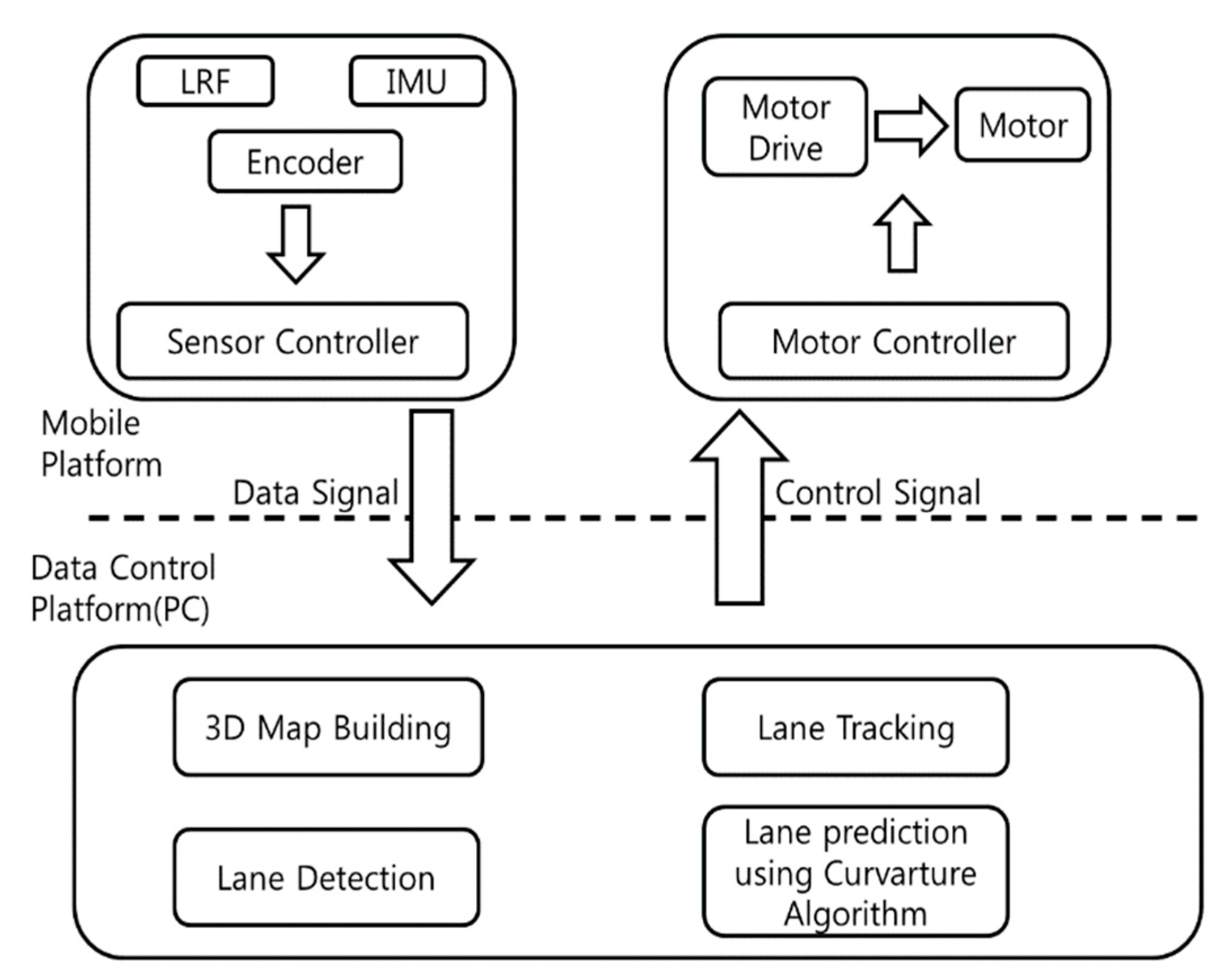
2. System Structure
3. Principles of LRF and 3D Map Building
3.1. Principle of LRF Lane Scanning
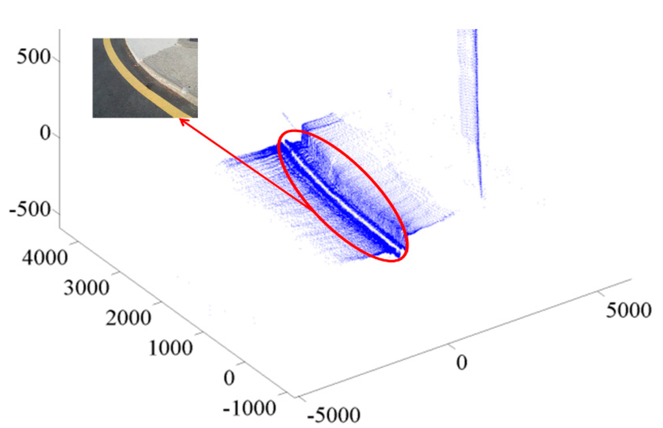
3.2. 3D Map Building
4. Lane Recognition and Prediction
4.1. Lane Feature Point Extraction
4.2. Curvature Algorithm

4.3. Limitations of Mobile Robot
4.4. Lane Tendency and Lane Prediction Using a Curvature Algorithm
4.5. Path Monitoring through Update
5. Tracking Control Algorithm
6. Experiment
6.1. Comparison Using Vision
6.2. Stable Tracking Algorithm Using Lane Tracking
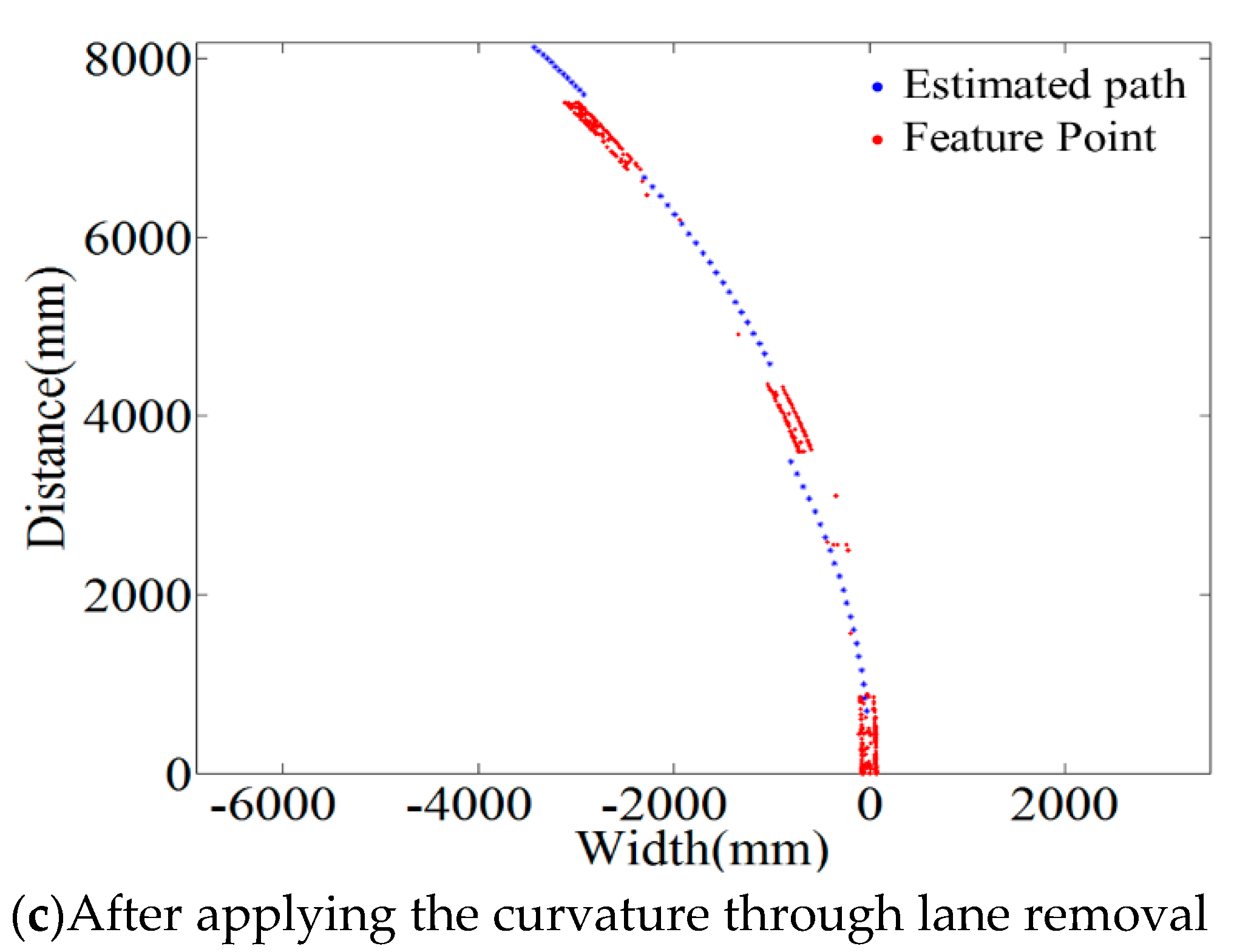
6.3. Lane Prediction Using the Curvature Algorithm
7. Conclusions
Author Contributions
Funding
Data Availability Statement
Conflicts of Interest
References
- Sparbert, J.; Dietmayer, K.; Streller, D. Lane detection and street type classification using laser range images. In Proceedings of the 2001 IEEE Intelligent Transportation Systems, Proceedings (Cat. No. 01TH8585), Oakland, CA, USA, 25–29 August 2001. [Google Scholar]
- Kim, Y.J.; Lee, K.B. Lateral Control of Vision-Based Autonomous Vehicle Using Neural Network; Korea Society for Precision Engineering: Seoul, Korea, 2000. [Google Scholar]
- Kim, S.-H.; Kim, M.-J.; Kang, S.-C.; Hong, S.-K.; Roh, C.-W. Development of Patrol Robot using DGPS and Curb Detection. J. Control. Autom. Syst. Eng. 2007, 13, 140–146. [Google Scholar] [CrossRef][Green Version]
- Pan, Z.; Chen, H.; Li, S.; Liu, Y. Cluster Map Building and Relocalization in Urban Environments for Unmanned Vehicles. Sensors 2019, 19, 4252. [Google Scholar] [CrossRef]
- Jung, J.-W.; Park, J.-S.; Kang, T.-W.; Kang, J.-G.; Kang, H.-W. Mobile Robot Path Planning Using a Laser Range Finder for Environments with Transparent Obstacles. Appl. Sci. 2020, 10, 2799. [Google Scholar] [CrossRef]
- Jiang, G.; Yin, L.; Liu, G.; Xi, W.; Ou, Y. FFT-Based Scan-Matching for SLAM Applications with Low-Cost Laser Range Finders. Appl. Sci. 2018, 9, 41. [Google Scholar] [CrossRef]
- Kluge, K.; Lakshmanan, S. A deformable-template approach to lane detection. In Proceedings of the Intelligent Vehicles ’95. Symposium, Detroit, MI, USA, 25–26 September 1995. [Google Scholar]
- Serge, B.; Michel, B. Lane Detection for Automotive Sensor. JCASSP 1995, 5, 2955–2958. [Google Scholar]
- Dickmanns, E.D.; Graefe, V. Dynamic Monocularmachine Vision and Application of Dynamic Monocular Vision. Int. J. Mach. Vis. Appl. 1988, 1, 223–240. [Google Scholar] [CrossRef]
- Kreucher, C.; Lakchmanan, S. LANA: A lane extraction algorithm that uses frequency domain features. IEEE Trans. Robot. Autom. 1999, 15, 343–350. [Google Scholar] [CrossRef]
- Risack, R.; Klausmann, P.; Kruger, W.; Enkelmann, W. Robust Lane Recognition Embedded in a Real-Time Driver Assistance System. In Proceedings of the Intelligent Vehicles Symposium, Stuttgart, Germany, 28–30 October 1998; IEEE Press: Piscataway, NJ, USA, 1998; Volume 1, pp. 35–40. [Google Scholar]
- Wang, Y.; Shen, D.; Teoh, E.K. Lane Detection using Catmull-Rom Spline. In Proceedings of the Intelligent Vehicles Symposium, Stuttgart, Germany, 28–30 October 1998; IEEE Press: Piscataway, NJ, USA, 1998; Volume 1, pp. 51–57. [Google Scholar]
- Suh, S.B.; Kang, Y.; Roh, C.-W.; Kang, S.-C. Experiments of Urban Autonomous Navigation using Lane Tracking Control with Monocular Vision. J. Inst. Control. Robot. Syst. 2009, 15, 480–487. [Google Scholar]
- Eun, S. Enhancing the Night Time Vehicle Detection for Intelligent Headlight Control using Lane Detection. In Proceedings of the KSAE 2011 Annual Conference, Topeka, KS, USA, 8–9 December 2011. [Google Scholar]
- Montremerlo, M.; Beeker, J.; Bhat, S.; Dahlkamp, H. The Stanford Entry in the Urban Challenge. J. Field Robot. 2008, 7, 468–492. [Google Scholar]
- Chun, C.-M.; Suh, S.-B.; Lee, S.-H.; Roh, C.-W.; Kang, S.-C.; Kang, Y.-S. Autonomous Navigation of KUVE (KIST Unmanned Vehicle Electric). J. Inst. Control. Robot. Syst. 2010, 16, 617–624. [Google Scholar] [CrossRef]
- Jung, B.-J.; Park, J.-H.; Kim, T.-Y.; Kim, D.-Y.; Moon, H.-P. Lane Marking Detection of Mobile Robot with Single Laser Rangefinder. J. Inst. Control. Robot. Syst. 2011, 17, 521–525. [Google Scholar] [CrossRef]
- Hiroi, Y.; Ito, A. A Pedestrian Avoidance Method Considering Personal Space for a Guide Robot. Robotics 2019, 8, 97. [Google Scholar] [CrossRef]
- Ali, M.A.; Mailah, M.; Jabbar, W.A.; Moiduddin, K.; Ameen, W.; Alkhalefah, H. Autonmous Road Roundabout Detecion and Navigation System for Smart Vehicles and Cities Using Laser Simulator-Fuzzy Logic Algorithms and Sensor Fusion. Sensors 2020, 20, 3694. [Google Scholar] [CrossRef] [PubMed]
- Li, L.; Luo, W.; Wang, K.C.P. Lane Marking Detection and Reconstruction with Line-Scan Imaging Data. Sensors 2018, 18, 1635. [Google Scholar] [CrossRef] [PubMed]
- Assuncao, A.N.; Aquino, A.L.L.; Santos, R.C.C.D.M.; Guimaraes, R.L.M.; Oliveira, R.A.R. Vehicle Driver Monitoring through the Statistical Process Control. Sensors 2019, 19, 3059. [Google Scholar] [CrossRef]
- Cao, J.; Song, C.; Song, S.; Xiao, F.; Peng, S. Lane Detection Algorithm for Intelligent Vehicles in Complex Road Conditions and Dynamic Environments. Sensors 2019, 19, 3166. [Google Scholar] [CrossRef] [PubMed]
- Hoang, V.-D.; Jo, K.-H. A Simplified Solution to Motion Estimation Using an Omnidirectional Camera and a 2-D LRF Sensor. IEEE Trans. Ind. Inform. 2016, 12, 1064–1073. [Google Scholar] [CrossRef]
- DU, X.; Tan, K.K. Comprehensive and Practical Vision System for Self-Driving Vehicle Lane-Level Localization. IEEE Trans. Image Process. 2016, 25, 2075–2088. [Google Scholar] [CrossRef] [PubMed]
- Wang, H.; Wang, Y.; Zhao, X.; Wang, G.; Huang, H.; Zhang, J. Lang Detection of Curving Road for Structural High-way with Straight-curve Model on Vision. IEEE Trans. Veh. Technol. 2019, 68, 5321–5330. [Google Scholar] [CrossRef]
- Dai, K.; Wang, Y.; Ji, Q.; Du, H.; Yin, C. Multiple Vehicle Tracking Based on Labeled Multiple Bernoulli Filter Using Pre-Clustered Laser Range Finder Data. IEEE Trans. Veh. Technol. 2019, 68, 10382–10393. [Google Scholar] [CrossRef]
- SICK. Available online: http://www.sick.com (accessed on 25 October 2019).
- Hokuyo Automatic Co., Ltd. Available online: http://www.hokuyo-aut.co.jp (accessed on 25 October 2019).
- Kawata, H.; Miyachi, K.; Hara, Y.; Ohya, A.; Yuta, S. A method for estimation of lightness of objects with intensity data from SOKUIKI sensor. In Proceedings of the IEEE International Conference on Multisensor Fusion and Integration for Intelligent Systems, Seoul, Korea, 20–22 August 2008; pp. 661–664. [Google Scholar] [CrossRef]
- Kawata, H.; Ohya, A.; Yuta, S.; Santosh, W.; Mori, T. Development of ultra-small lightweight optical range sensor system. In Proceedings of the 2005 IEEE/RSJ International Conference on Intelligent Robots and Systems, Edmonton, AB, Canada, 2–6 August 2005; pp. 1078–1083. [Google Scholar] [CrossRef]
- Zhu, J.; Ahmad, N.; Nakamoto, H.; Matsuhira, N. Feature Map Building Based on Shape Similarity for Home Robot ApriAtenda. In Proceedings of the 2006 IEEE International Conference on Robotics and Biomimetics; Institute of Electrical and Electronics Engineers (IEEE), Kunming, China, 17–20 December 2006; pp. 1030–1035. [Google Scholar]
- Jia, S.; Yang, H.; Li, X.; Fu, W. LRF-based data processing algorithm for map building of mobile robot. In Proceedings of the 2010 IEEE International Conference on Information and Automation, Harbin, China, 20–23 June 2010; pp. 1924–1929. [Google Scholar]
- Grossman, S.I.; Derrick, W.R. Advanced Engineering Mathematics; Harper Collins Publishers: New York, NY, USA, 2000. [Google Scholar]
- Dudek, G.; Jenkin, M. Computational Principles of Mobile Robotics; Cambridge University Press (CUP): Cambridge, UK, 2009. [Google Scholar]
- Kim, M.S.H.; Han, J.; Lee, J. Optimal Trajectory Control for Capturing a Mobile Sound Source by a Mobile Robot. Int. J. Hum. Robot. 2017, 14, 1750025. [Google Scholar] [CrossRef]
- Han, J.-H. Tracking Control of Moving Sound Source Using Fuzzy-Gain Scheduling of PD Control. Electronics 2019, 9, 14. [Google Scholar] [CrossRef]
- Kanayama, Y.; Kimura, Y.; Miyazaki, F.; Noguchi, T. A stable tracking control method for an autonomous mobile robot. In Proceedings of the IEEE International Conference on Robotics and Automation, Washington, DC, USA, 11–15 May 2002; Volume 1, pp. 384–389. [Google Scholar] [CrossRef]


| UBG-04LX | Light Source | Semiconductor laser diode (785 nm) Laser safety Class1 (IEC60825-1) |
| Detection Distance Standard Object | Accuracy Range: 60~4095 mm Square Kent Sheet 80 mm | |
| Detection Distance /Scan Angle | 20~4000 mm/240° | |
| Resolution/ Angular Resolution | 1 mm/0.36°(360°/1024 steps) | |
| Scan Time | 100 msec/scan | |
| Interface | RS-232C (19.2, 57.6, 115.2, 500, 750 kbps) USB 2.0 (Full Speed) |
| IMU (EBINU-9DOF) | Input Voltage | 5 V |
| Current | 40 mA | |
| Data Output Velocity | 1~100 Hz | |
| Sensitivity | Gyro: 250~2000 dps Acceleration: 2~8 g Compasses:1.3~8.1 gauss | |
| Resolution | 0.01 degree | |
| Size (L, W) | 15 mm, 23.5 mm | |
| Interfaces | TTL Level (3.3 V) Serial Communication |
| Motor (RB35GM) | Rated Voltage | 12 V |
| Rated Torque | 2.0 g-cm | |
| Rated Speed | 102 rpm | |
| Output Power | 3.14 W | |
| Deceleration | 50:1 | |
| Motor Driver (NT-S-DCDM1210) | Input Voltage Range | 12~24V |
| Maximum Continuous Current | 5 A | |
| PWM Frequency | 14.4 Khz | |
| Interface | RS-232, I2C |
| Controller (Mycortex-LM8962) | Power | 3.3 V |
| Clock | 50 Mhz | |
| Memory | 256 kB flash/64 kB SRAM | |
| Product Features | 32-Bit RISC, GPT, SSI, UART, ADC, I2C, PWM, GPIO |
| Max (mm) | Mean (mm) | Max Error (mm) | |
|---|---|---|---|
| Real lane | - | 150 | - |
| LRF-scanned lane | 169 | 104 | 19 mm (12.7%) |
Publisher’s Note: MDPI stays neutral with regard to jurisdictional claims in published maps and institutional affiliations. |
© 2021 by the authors. Licensee MDPI, Basel, Switzerland. This article is an open access article distributed under the terms and conditions of the Creative Commons Attribution (CC BY) license (https://creativecommons.org/licenses/by/4.0/).
Share and Cite
Han, J.-H.; Kim, H.-W. Lane Detection Algorithm Using LRF for Autonomous Navigation of Mobile Robot. Appl. Sci. 2021, 11, 6229. https://doi.org/10.3390/app11136229
Han J-H, Kim H-W. Lane Detection Algorithm Using LRF for Autonomous Navigation of Mobile Robot. Applied Sciences. 2021; 11(13):6229. https://doi.org/10.3390/app11136229
Chicago/Turabian StyleHan, Jong-Ho, and Hyun-Woo Kim. 2021. "Lane Detection Algorithm Using LRF for Autonomous Navigation of Mobile Robot" Applied Sciences 11, no. 13: 6229. https://doi.org/10.3390/app11136229
APA StyleHan, J.-H., & Kim, H.-W. (2021). Lane Detection Algorithm Using LRF for Autonomous Navigation of Mobile Robot. Applied Sciences, 11(13), 6229. https://doi.org/10.3390/app11136229