Article

A Study of Predictive Models for Early Outcomes of Post-Prostatectomy Incontinence: Machine Learning Approach vs. Logistic Regression Analysis Approach

1
Machine Intelligence Laboratory, Department of Smart Automobile, Soonchunhyang University, Asan, Chungcheongnamdo 31538, Korea
2
Department of Radiology, Hallym University College of Medicine, Kangnam Sacred Heart Hospital, Seoul 07441, Korea
3
Department of Radiology, College of Medicine, Ewha Womans University, Seoul 07804, Korea
*
Author to whom correspondence should be addressed.
Appl. Sci. 2021, 11(13), 6225; https://doi.org/10.3390/app11136225
Submission received: 26 May 2021 / Revised: 26 June 2021 / Accepted: 29 June 2021 / Published: 5 July 2021

Abstract

:
Background: Post-prostatectomy incontinence (PPI) is a major complication that can significantly decrease quality of life. Approximately 20% of patients experience consistent PPI as long as 1 year after radical prostatectomy (RP). This study develops a preoperative predictive model and compares its diagnostic performance with conventional tools. Methods: A total of 166 prostate cancer patients who underwent magnetic resonance imaging (MRI) and RP were evaluated. According to the date of the RP, patients were divided into a development cohort (n = 109) and a test cohort (n = 57). Patients were classified as PPI early-recovery or consistent on the basis of pad usage for incontinence at 3 months after RP. Uni- and multi-variable logistic regression analyses were performed to identify associates of PPI early recovery. Four well-known machine learning algorithms (k-nearest neighbor, decision tree, support-vector machine (SVM), and random forest) and a logistic regression model were used to build prediction models for recovery from PPI using preoperative clinical and imaging data. The performances of the prediction models were assessed internally and externally using sensitivity, specificity, accuracy, and area-under-the-curve values and estimated probabilities and the actual proportion of cases of recovery from PPI within 3 months were compared using a chi-squared test. Results: Clinical and imaging findings revealed that age (70.1 years old for the PPI early-recovery group vs. 72.8 years old for the PPI consistent group), membranous urethral length (MUL; 15.7 mm for the PPI early-recovery group vs. 13.9 mm for the PPI consistent group), and obturator internal muscle (18.2 mm for the PPI early-recovery group vs. 17.5 mm for the PPI consistent group) were significantly different between the PPI early-recovery and consistent groups (all p-values < 0.05). Multivariate analysis confirmed that age (odds ratio = 1.07, 95% confidence interval = 1.02–1.14, p-value = 0.007) and MUL (odds ratio = 0.87, 95% confidence interval = 0.80–0.95, p-value = 0.002) were significant independent factors for early recovery. The prediction model using machine learning algorithms showed superior diagnostic performance compared with conventional logistic regression (AUC = 0.59 ± 0.07), especially SVM (AUC = 0.65 ± 0.07). Moreover, all models showed good calibration between the estimated probability and actual observed proportion of cases of recovery from PPI within 3 months. Conclusions: Preoperative clinical data and anatomic features on preoperative MRI can be used to predict early recovery from PPI after RP, and machine learning algorithms provide greater diagnostic accuracy compared with conventional statistical approaches.

1. Introduction

Post-prostatectomy incontinence (PPI) is a significant functional complication that can negatively affect a patient’s quality of life following radical prostatectomy (RP) [1,2,3]. Although improved surgical techniques have been introduced, the incidence of PPI remains high, particularly during the early postoperative period [1]. Approximately 20% of patients experience consistent PPI as long as 1 year after RP [4]. In addition to surgical techniques, various demographic and anatomical factors reportedly influence PPI recovery [5,6,7,8,9,10,11,12,13]. Advanced age, high body mass index (BMI), a large prostate size and shape, the presence of comorbidities, a history of transurethral resection of the prostate (TURP), or a history of lower urinary tract symptoms have been associated with delayed continence recovery [14,15]. Surgical factors, including surgery type and neurovascular bundle-sparing, are also associated with recovery rates from PPI [16]. Regarding anatomic features, previous studies have reported that preoperative membranous urethral length (MUL), which is related to urethral sphincter function, is strongly associated with PPI after RP [6,7,17]. Other anatomical pelvic structures around the urethra and postoperative bladder neck sparing have shown potential as predictors for recovery from PPI [5,18,19]. While multiple related factors are known, a complex relationship among them makes it difficult to predict an individual’s likelihood of recovery from PPI, and there is a paucity of reports on predictive models for recovery from PPI following RP [16,20].
In recent years, machine learning approaches have become popular tools for constructing prediction models in medicine, primarily in complex multi-variable systems [21,22]. Magnetic resonance imaging (MRI) is now a standard method for detecting significant prostate cancer using the Prostate Imaging–Reporting and Data System [23]. The diagnostic value of MRI means it can be used to delineate the anatomic pelvic structure around the urethra, preoperatively.
Here, we describe a system to predict early recovery from PPI using machine learning algorithms and compared its diagnostic performance with that of conventional logistic regression (LR) using only preoperative clinical data and preoperative anatomical features.

2. Materials and Methods

2.1. Patients

This study was approved and exempted from informed consent by the Institutional Review Board of Kangnam Sacred Heart Hospital (2021-03-004). We reviewed the records of 284 consecutive patients pathologically diagnosed with prostate cancer between July 2016 and December 2019. Of these patients, we identified 185 who underwent preoperative MRI and RP at our institution. After excluding 19 patients who met the following exclusion criteria: inadequate imaging quality for assessment (n = 6), inadequate clinical follow-up period (n = 8), and unavailable information of consistent status (n = 5), 166 patients were enrolled in our study. According to the date of RP, the 166 patients were divided into development and test cohorts; the 109 patients who underwent RP from July 2016 to August 2018 were assigned to the development cohort to generate a prediction model, and the 57 patients who underwent RP from September 2018 to December 2019 were assigned to the test cohort [24].
Clinical and demographic characteristics of all study participants, such as age, initial prostate-specific antigen (PSA) level, history of TURP, biopsy Gleason score, BMI, and surgery type (open, laparoscopic and robotic RP), were collected from electronic medical records (EMRs).

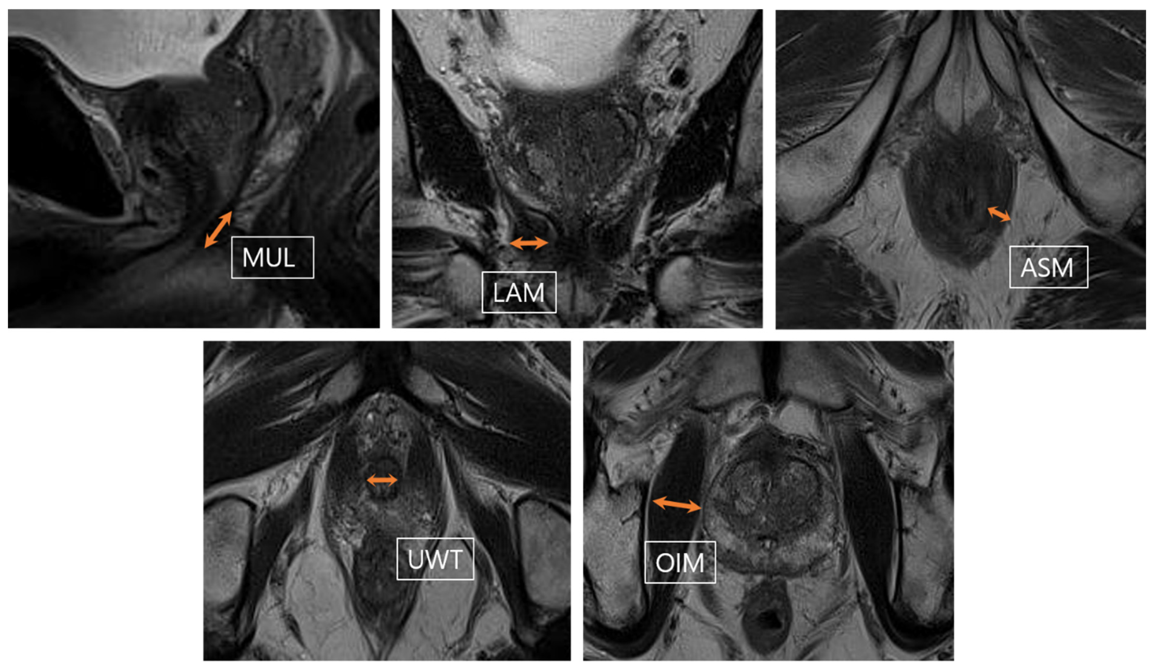
2.2. Magnetic Resonance Images and Measurements

Preoperative MRI examinations were obtained using 3-T MRI scanners (Skyra, Siemens Healthcare). An intramuscular injection of 40 mg of intramuscular butylscopolamine bromide (Buscopan; Boehringer Ingelheim, Ingelheim, Germany) was administered to prevent spasms. The MRI protocol included axial, sagittal, and coronal T2-, axial T1- and single-shot echo-planar digital weighted imaging, apparent diffusion coefficient mapping, and dynamic contrast enhanced imaging.
The preoperative prostate volume (PV), MUL, levator ani muscle (LAM), urethra wall thickness (UWT), anal sphincter muscle (ASM), and obturator internal muscle (OIM) were measured using MRI (Figure 1). PV was calculated using the following formula: height (cm) × length (cm) × width (cm) × π/6 [23]. MRI measurements were performed by a board-certified radiologist (BJ) with >8 years of experience in interpreting prostate MRI scans who was blinded to clinical information.

2.3. Assessment of Incontinence

We investigated the patients’ continence status retrospectively from using EMRs at a 3 months’ follow-up after RP at our institution. Urinary incontinence status was assessed based on patient-reported daily pad usage for leakage control over the past 4 weeks and the Expanded Prostate Cancer Indexed Composite urinary assessment [25]. Patients who did not wear pads or wore an occasional security pad were assigned to the early-recovery group; otherwise they were assigned to the consistent PPI group. The patients who reported wearing a security pad due to slight leakage were considered subjects who used one pad daily and were added to the consistent group [16].

2.4. Data Split for Model Development and Testing

To show that small data are not biased, test data must not be used for learning at all, so we divided the dataset into temporal parts to construct these datasets [26]. So, as we talked in Section 2.1, the 166 patients were divided into two groups, development and test cohorts; the 109 patients from July 2016 to August 2018 were assigned to the development cohort to generate a prediction model, and the 57 patients from September 2018 to December 2019 were assigned to the test cohort. The development cohort data were used for the training machine learning algorithm to predict PPI-recovery and test data were used for verifying our proposed method [27].

2.5. Building Process of Prediction Models Using Machine Learning Algorithms

We developed a PPI-recovery prediction model using several established machine learning algorithms: k-nearest neighborhood (KNN), decision tree (DT), random forest (RF) and support-vector machine (SVM) [28,29] in Appendix A. As we mentioned in Section 2.3, development cohort data were used for building a machine learning model. In general, machine learning algorithms may be able to occur overfitting problems that are optimized for training data in the training process, so various techniques have been introduced to prevent such methods, such as using a validation dataset. In this paper, we used an automatic hyper parameter tuning tool in the statistical machine learning toolbox, MATLAB 2020b [30]. The automatic hyper-parameter tuning method of MATLAB 2020b alters the hyper-parameter to find a hyper-parameter that minimizes the cross-validation loss (error) for the prediction results of machine learning, and performs the optimization of the hyper-parameter as well. In other words, in this paper, we used an auto hyper-parameter tuning tool which has the same effect as utilizing the validation set to prevent overfitting, which were to be optimized only for the development cohort datasets. The Hyper-parameter optimization tool also uses several methods to find optimal parameters, among these methods in this paper we utilized the grid search method. The grid search method divides the dimension of the hyper-parameter into several grids, selecting one representative hyper-parameter for each grid, and then selects the best performing parameter and grid. In the same way, the best performing grid is divided into several grids to continuously find the best grid of the selected hyper-parameter.
The final prediction model is represented by an internal performance validated by applying to the development cohort and external performance validated by applying to the test cohort. The below Table 1 shows the parameters optimized by the hyper-optimization tool for each machine learning algorithm.
We validated the performance of our proposed prediction model using the development cohort data and test cohort data. First, we divided the development cohort data randomly by a ratio of 9 to 1, then performed the training with 9 part data, validated the internal performance with 1 part data, and validated the external performance with the test cohort data. We performed these tasks a total of 10 iterations repeatedly to analyze the performance with the mean and standard deviation of the internal/external ROC.

2.6. Statistical Analysis

Data were compared with a Student’s t-test or a nonparametric Mann–Whitney U test for continuous variables, and a chi-squared test Fisher’s exact test for categorical variables, as appropriate. Uni- and multivariate LR analyses were performed to determine the associated factors for recovery from PPI within 3 months after RP. These statistical analyses were performed using SPSS (version 21.0; SPSS, Inc., Chicago, IL, USA). A p-value < 0.05 was considered statistically significant. The predictive model for recovery from PPI within 3 months after RP was developed using MATLAB 2020b with the Statistical Machine and Deep Learning toolboxes. The accuracy, sensitivity, specificity, and area under the receiver operating characteristic curve were evaluated to determine the performance of several predictive models using the various algorithms. A chi-squared test was used to evaluate the agreement between the estimated probability and actual observed proportion of cases of recovery from PPI within 3 months.

3. Results

3.1. Subsection Baseline Characteristics of the Development and Test Cohorts

Baseline characteristics of the 109 development patients (mean age, 71.9 ± 6.4 years) and 57 test patients (mean age, 71.0 ± 7.3 years) are described in Table 2. Recovery from PPI was achieved in 51.4% of the cases within 3 months after RP in the development group, and in 35.1% of the test group, respectively. The rate of recovery from incontinence within 3 months was significantly lower in the test group (p = 0.045). Surgical methods and MRI measurements, including MUL and OIM, between the two groups were significantly different (p < 0.05).

3.2. Comparison between PPI Early-Recovery and Consistent Group and Logistic Regression Analysis

Characteristics of PPI early-recovery and consistent groups within 3 months after RP are provided in Table 3. Early-recovery patients within 3 months were significantly older than the PPI consistent patients (70.1 versus 72.8 years old; p = 0.009). In the anatomic findings from MRI, MUL (15.7 versus 13.9 mm; p = 0.002) and OIM (18.2 versus 17.5; p = 0.021) were significantly longer and thicker with early-recovery patients than those of consistent patients.
Univariate logistic regression analysis showed that age (odds ratio (OR), 1.06; 95% confidence interval (CI) 1.01–1.12; p = 0.011) and MUL (OR, 0.88; 95% CI 0.81–0.96; p = 0.003) were significantly related with PPI recovery within 3 months. In multivariate logistic regression analysis, both age (OR, 1.07; 95% CI 1.07–1.02; p = 0.007) and MUL (OR, 0.87; 95% CI 0.80–0.95; p = 0.002) remained significant independent predictors of PPI recovery within 3 months after RP (Table 4).

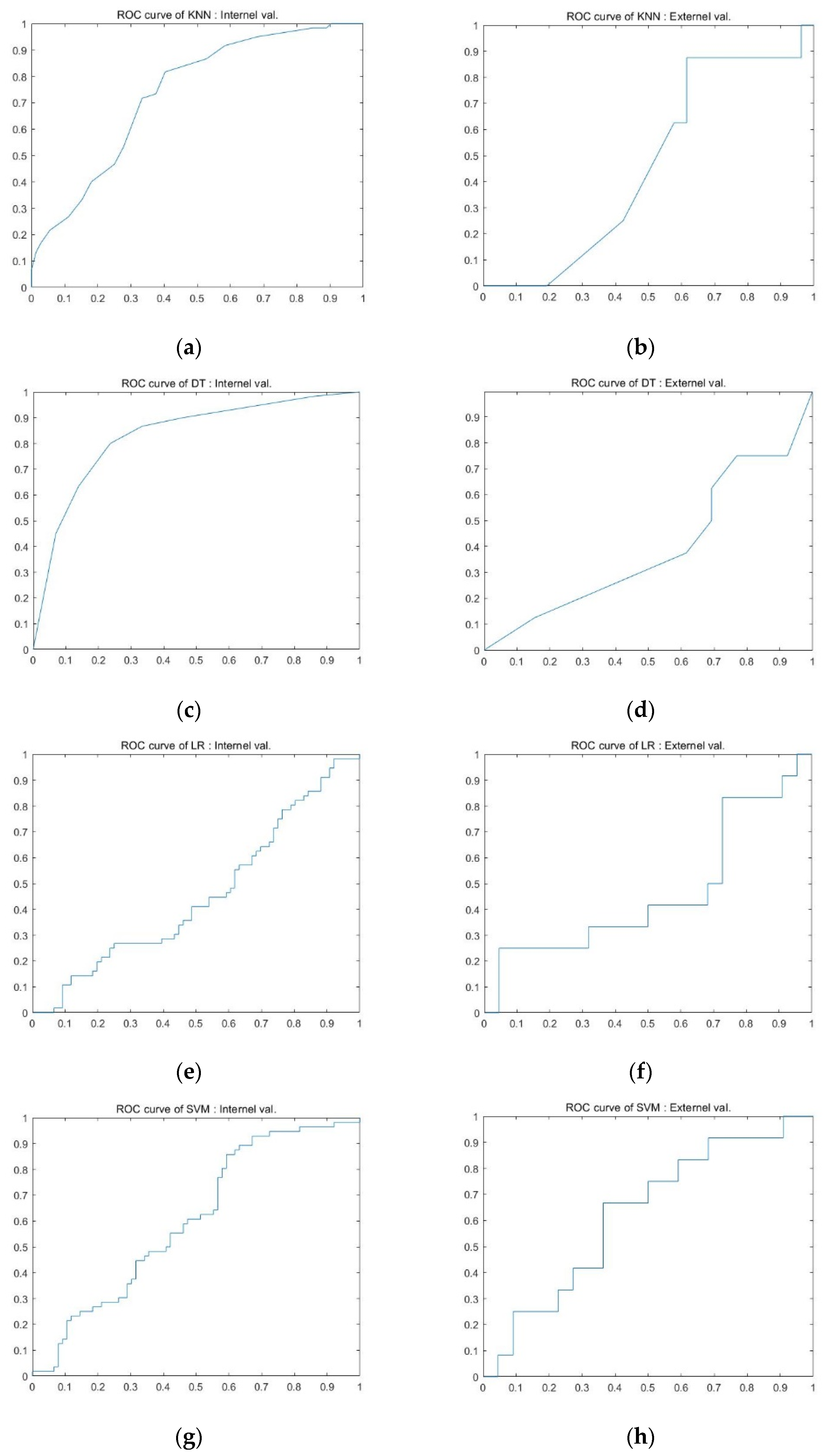
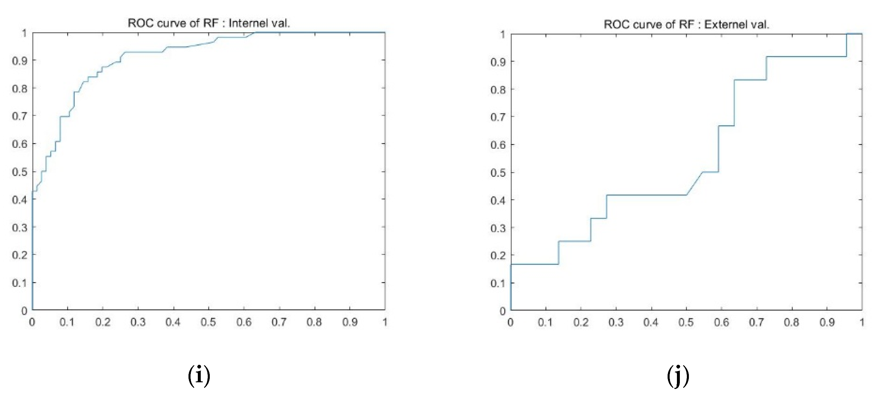
3.3. Diagnostic Performance of the Predictive Models

The diagnostic performance of each model is provided in Table 5, Table A1 in Appendix B and Figure 2. The AUCs were 0.63 ± 0.04 for LR, 0.73 ± 0.09 for KNN, 0.73 ± 0.09 for DT, 0.72 ± 0.03 for SVM, and 0.80 ± 0.1 for RF in the internal validation group, representing improved performance from LR over the machine learning model. In the external validation group, four machine learning models had AUCs of 0.60 ± 0.08 for KNN, 0.61 ± 0.07 for DT, 0.65 ± 0.07 for SVM, and 0.61 ± 0.08 for RF. Among them, SVM yielded improved discrimination compared with LR (0.59 ± 0.07). Chi-squared tests for all models showed that the estimated probability of PPI within 3 months did not differ from the actual observed proportion of recovery from PPI within 3 months (p > 0.05).

4. Discussion

This current study presents a preoperative predictive model for early recovery from PPI within 3 months after RP. Age, MUL, and OIM were significantly different between the early-recovery group and the consistent group. In multivariate LR analyses, age and MUL were significant independent factors. Based on these results, a predictive model with LR analysis showed low to moderate diagnostic accuracy. Applying a machine learning algorithm, the predictive models showed improved diagnostic performance with higher AUCs compared with the model using LR, especially in the SVM algorithm. These models showed a good calibration between the estimated probability actual proportion of cases experiencing early recovery from PPI.
Previous studies have suggested that older age, a higher BMI, the coexistence of medical comorbidities, a history of TURP, the presence of preoperative lower urinary tract symptoms, decreased MUL, surgery type, PV, and sacrificed neurovascular bundles may be risk factors for urinary incontinence after RP [14,16,17,31,32,33]. Among them, we focused on the preoperative factors and the measurements of pelvic skeletal muscles using MRI. Determining the preoperative factors related to the consistent status after RP and patients at a high risk of incontinence would be of value to clinicians when consulting patients prior to surgery and in explaining delays in postoperative urinary incontinence recovery. In the current study, the probability of continence recovery within 3 months after RP increased with MUL and decreased with age. A previous study found that maximal urethral closure decreased by approximately 27% after RP [34]. Patients with a longer MUL were more likely to maintain a longer intact urethra sphincter and, subsequently, a higher urethral closure pressure after RP [35]. In other words, a longer MUL was more likely to maintain sphincter function. Our results are consistent with previous findings of a significant relationship between MUL and continence recovery after RP. Age has been confirmed as a significant factor influencing a consistent status after RP [6,7,18,30,36,37]. According to a study by Nilsson et al., a patient’s age at RP influenced the risk of incontinence in an exponential manner, particularly in long-term urinary incontinence [37]. Another study found that an age < 70 years was highly relevant to recovery from PPI within 3 months after RP [36]. This finding could be due to a general loss of ability to control urination with age.
Concerning the complicated physiology of micturition involving various organs and the nervous system, it appears to be difficult to predict the status of continence after RP. Several intraoperative maneuvers have been also shown to affect continence states following post-prostatectomy, including neurovascular bundle-sparing surgery [34,38,39], bladder neck preservation [40], and novel reconstruction of tissue around the vesicourethral anastomosis [41]. Additionally, the surgeons’ experience and skill are also involved in urinary outcomes after RP [42]. Accordingly, surgical technique could be individually tailored, especially for high-risk patients with PPI. In addition to changing surgical techniques, preoperative machine learning-based predictive models are useful for preoperative and postoperative patient counseling and postoperative treatment planning. Conservative treatments such as pelvic floor exercises, behavior modifications, pelvic floor stimulation, and biofeedback to relieve urinary incontinence can be administered to high-risk patients at an early stage, and unnecessary aggressive surgical correction can be avoided for patients who can expect to recover from PPI. In the current study, when a traditional LR model was used, the diagnostic performance of predictive PPI early-recovery yielded low to moderate accuracy, with an AUC of 0.63 in an internal validation group and 0.59 in an external validation group. Machine learning has been increasingly employed for precise diagnosis and prediction of outcomes [43]. This approach offers the advantage of analyzing clinical practice data with numerous confounding factors and associated factors that are closely and intricately related to each other. By using machine learning algorithms, the AUC significantly improved to 0.73 with KNN, 0.73 with DT, 0.72 with SVM, and 0.81 with RF in an interval validation group and to 0.60 with KNN, 0.61with DT, 0.65 with SVM, and 0.61 with RF in an external validation group, although the difference was only statistically significant with SVM. These results suggest that a machine learning approach exhibited superior, or at least comparable, performance compared with conventional statistical approaches in terms of predicting early recovery from PPI. In addition, these models showed good calibration, suggesting that these data are useful in determining early recovery from PPI within 3 months after RP.
This study had several limitations. First, it was vulnerable to selection bias due to the nature of its retrospective design. Other factors that can be expected to affect continence status after RP, such as the presence of preoperative lower urinary tract symptoms, were not evaluated. Second, this study was performed in a single institution with a small number of patients. We found significant improvements in diagnostic performance using machine learning algorithms in an internal validation group, but not in an external validation group, with the exception of the SVM. This may be due to the small number of events, warranting further study with a larger number of patients. Third, we used patient-reported daily pad usage to assess incontinence, which is a relatively subjective metric. However, a recent prospective multicenter study by Nitti et al. confirmed that the number of pads can accurately measure a patient’s post-prostatectomy incontinence [44]. Finally, as there were three surgeons in our institution during the study period, inevitable technical differences between surgeons may have biased the results.

5. Conclusions

Preoperative clinical data and anatomic features revealed by preoperative MRI can be used to predict early recovery from PPI after RP, and machine learning algorithms offer superior diagnostic accuracy compared with conventional statistical approaches. Our predictive model may be useful for personalized counseling for a post-prostatectomy consistent status before RP.

Author Contributions

Conceptualization, S.P. and J.B.; methodology, S.P. and J.B.; software, S.P.; validation S.P. and J.B.; formal analysis, S.P. and J.B.; investigation, J.B.; resources, S.P. and J.B.; data curation, J.B.; writing—original draft preparation, S.P. and J.B.; writing—review and editing, S.P. and J.B.; visualization, S.P. and J.B.; supervision, J.B.; project administration, J.B.; funding acquisition, S.P. Both authors have read and agreed to the published version of the manuscript.

Funding

This work was supported by Soonchunhyang University.

Institutional Review Board Statement

This study was approved and exempted from informed consent by the Institutional Review Board of Kangnam Sacred Heart Hospital (2021-03-004).

Informed Consent Statement

Informed consent was waived by the Institutional Review Board of Kangnam Sacred Heart Hospital due to the nature of the retrospective study design.

Data Availability Statement

Not applicable.

Acknowledgments

The authors thank the reviewers and editors in the Applied Science journal.

Conflicts of Interest

The authors declare no conflict of interest.

Appendix A

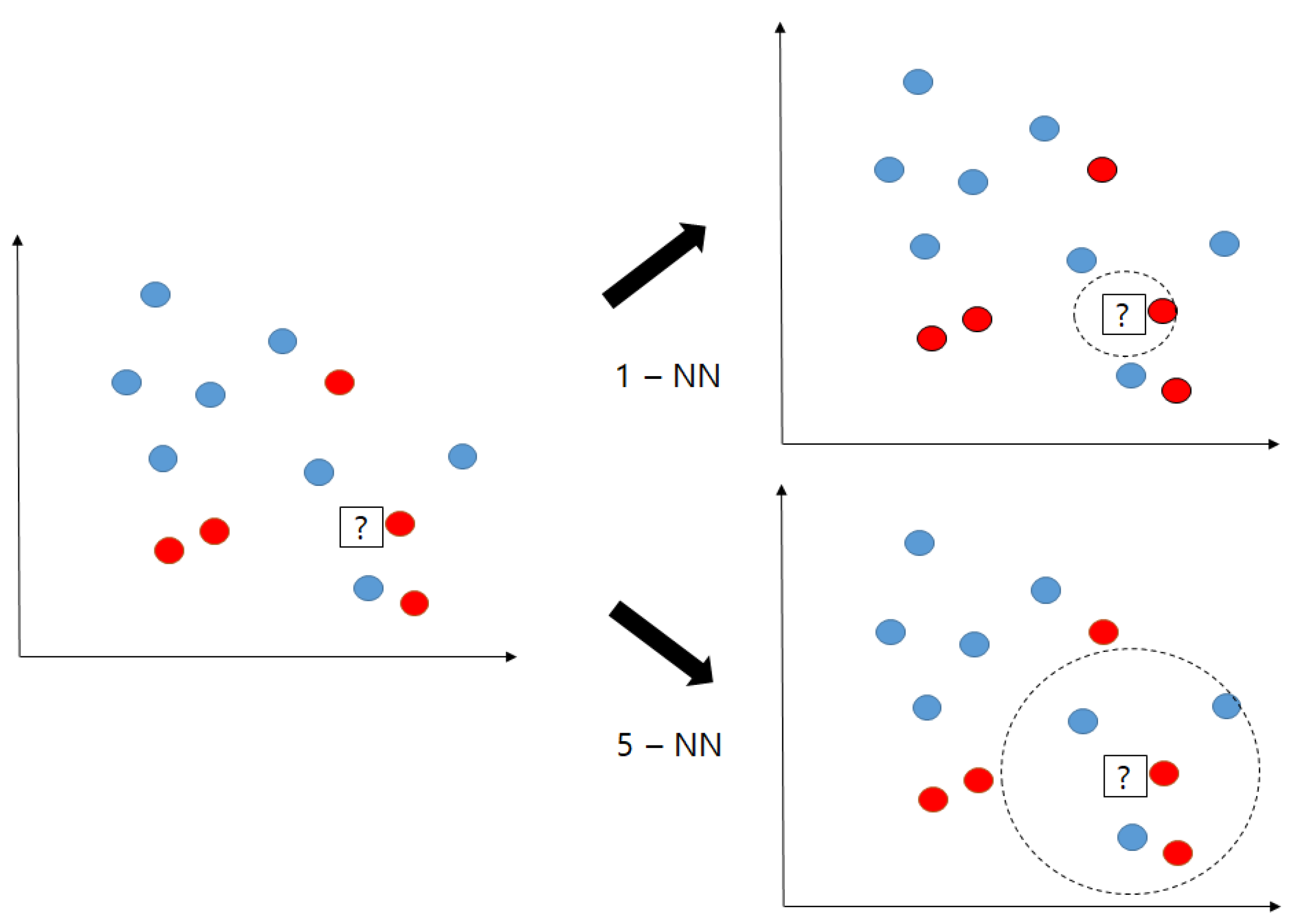
Appendix A.1. K-Nearest Neighborhood

A KNN [28] is a simple machine learning method for classification and regression. The output value of the test data is predicted by the output value of the nearest k training data from the test data. Figure A1 provides one example of a KNN: 1-NN and 5-NN.
Figure A1. Example of K-NN: 1-NN and 5-NN cases.
Applsci 11 06225 g0a1
In the 1-NN case, test data are predicted as a red circle because the nearest data point is the red circle; however, the 5-NN case test data are as classified as blue circles because more than half of the five closest data points are blue circles. Another important parameter in K-NN is the distance that determines which data are the closest. The most popular distance is measured between two data X = ( x 1 x 2 x n ) and Y = ( x 1 x 2 x n ) , where * i are features of the data as follows:
Euclidean :   d E u c l i d e a n = ( x i y i ) 2
Malanobis :   d M a h a l a n o b i s = ( X Y ) T Σ 1 ( X Y ) w h e r e   Σ   i s   c o v a r i a n c e   m a t r i x   b e t w e e n   X   a n d   Y  
Manhattan :   d M a n h a t t a n = | x i y i |
In this paper, we used 5-NN with the Euclidean distance to choose data that predict hepatic enhancement.

Appendix A.2. Decision Tree

A DT [29] is an intuitive and explainable machine learning algorithm for classification and regression. The training method is a classification and regression tree (CART) method that divides the data into two subsets depending on the characteristics that distinguish the data in the training set. The CART sets a threshold for one input feature, then divides the data into two subsets according to the threshold, and sets the input factor and its threshold to minimize the impurity of the two divided subsets. The cost function of the CART is described as Equation (A4):
J ( k , t k ) = m l e f t m G l e f t + m r i g h t m G r i g h t
where k is the kth feature of input, t k is the threshold of the kth feature of input, G l e f t / r i g h t is the impurity of the left/right subset, m l e f t / r i g h t is the number of samples of the left/right subset, and m is the whole number of the sample. The CART generates a tree structure using a recursive method of dividing subsets. There are two impurity criterion: Gini and Entropy, and in this paper we used the Gini method to determine the impurity of the subset tree.

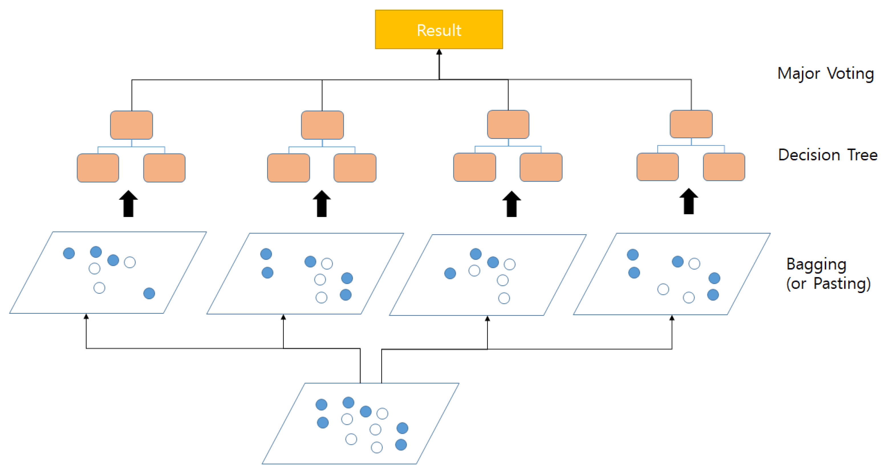
Appendix A.3. Random Forest

An RF [29] is an ensemble decision tree. An ensemble method achieves superior performance compared with a general machine learning algorithm because it is a parallel combination of multiple machine learning algorithms with different performances that fuse the results of each algorithm. The structure of a random forest is provided in Figure A2.
Figure A2. Structure of random forest.
Applsci 11 06225 g0a2
To implement a random forest comprising a number of decision trees, we used the bagging and pasting method. The random forest training method extracts a few data points from a training dataset, constructs a decision tree with the extracted data, and iterates these tasks to construct multiple trees. The training data extraction technique that allows redundancy is called bagging, and the technique that does not allow redundancy is called pasting. The final decision of the random forest uses primarily the major voting method, which selects the most-selected class among the multiple trees.

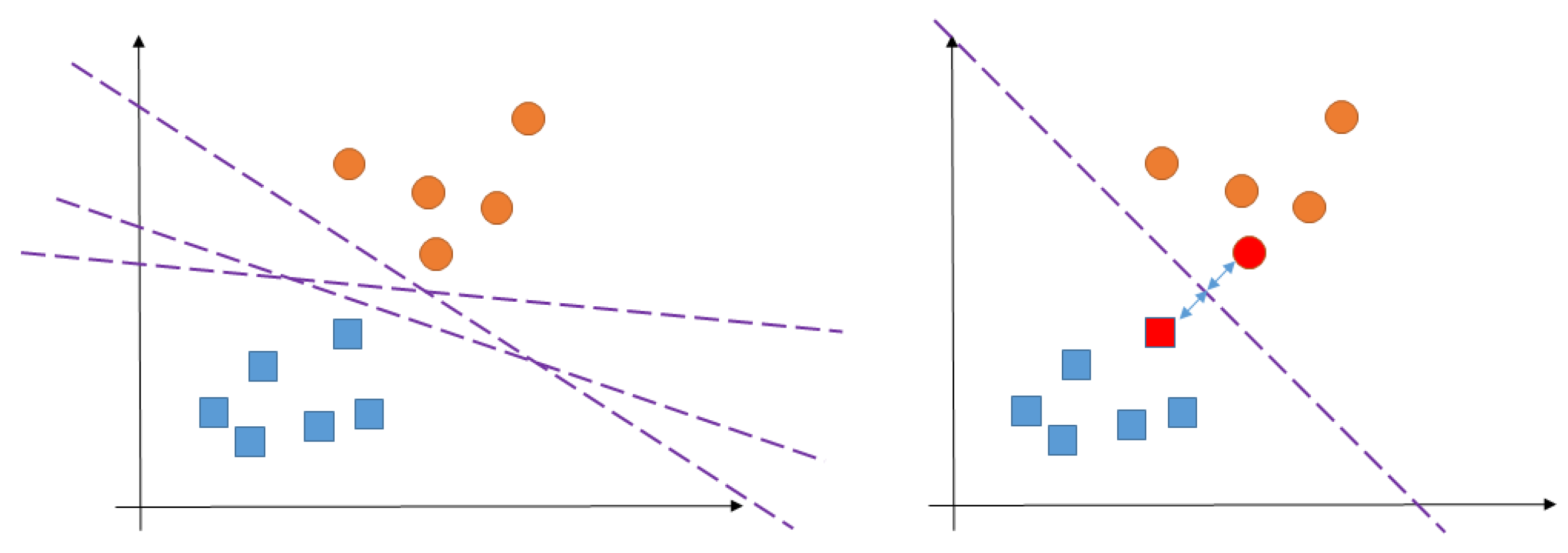
Appendix A.4. Support Vector Machine

An SVM [29] is a powerful and multi-purpose machine learning algorithm that can be used for classification, regression, and anomaly detection. Unlike a hyperplane, in which a typical linear classifier or neural network classifies two classes, hyperplanes in an SVM can drop the nearest samples between different classes the farthest away. The difference between a typical classifier (neural network) and an SVM is shown in Figure A3.
Figure A3. Hyperplanes of a classifier: typical algorithm (left), SMV (right).
Applsci 11 06225 g0a3
The decision function of the linear SVM is shown in Equation (A5) below:
y ^ = { 0   when   w T x + b < 0 1   when   w T x + b > 0
where x is the nth-dimension input and w and b are trainable weight and bias, respectively. If the output value of the SVM is greater than 0, it becomes a positive class, otherwise a negative class. In other words, the class is separated according to the value of the linear hyperplane by the decision function, as shown in Figure A3. However, a linear hyperplane cannot classify a class of samples when the data require nonlinear classification performance.
As only linear classification is applicable in a basic SVM, we used a kernel SVM to overcome this limitation. Equations (A6)–(A9) are the most widely used kernels in SVMs:
Linear :   K ( a , b ) = a T b
Polynomial :   K ( a , b ) = ( γ a T b + r ) d
RBF :   K ( a , b ) = exp ( γ a b )
Sigmoid :   K ( a , b ) = tanh ( γ a T b + r )

Appendix B

Table A1. The p-value for multiple comparisons for AUC of predictive models.
KNNDTSVMRFLR
Internal validation cohortKNN1.000----
DT0.9841.000---
SVM0.2250.1401.000--
RF0.001<0.001<0.0011.000-
LR<0.001<0.001<0.001<0.0011.000
External validation cohortKNN1.000----
DT0.8541.000---
SVM0.0020.0021.000--
RF0.5330.6310.0141.000-
LR0.3750.251<0.0010.1211.000

References

  1. Punnen, S.; Cowan, J.E.; Chan, J.M.; Carroll, P.R.; Cooperberg, M.R. Long-Term Health-Related Quality of Life after Primary Treatment for Localized Prostate Cancer: Results from the CaPSURE Registry. Eur. Urol. 2015, 68, 600–608. [Google Scholar] [CrossRef] [PubMed] [Green Version]
  2. Liss, M.A.; Osann, K.; Canvasser, N.; Chu, W.; Chang, A.; Gan, J.; Li, R.; Santos, R.; Skarecky, D.; Finley, D.S.; et al. Continence Definition after Radical Prostatectomy Using Urinary Quality of life: Evaluation of Patient Reported Validated Questionnaires. J. Urol. 2010, 183, 1464–1468. [Google Scholar] [CrossRef] [PubMed]
  3. Sanda, M.G.; Dunn, R.L.; Michalski, J.; Sandler, H.M.; Northouse, L.; Hembroff, L.; Lin, X.; Greenfield, T.K.; Litwin, M.S.; Saigal, C.S.; et al. Quality of Life and Satisfaction with Outcome among Prostate-Cancer Survivors. N. Engl. J. Med. 2008, 358, 1250–1261. [Google Scholar] [CrossRef]
  4. Ficarra, V.; Novara, G.; Rosen, R.C.; Artibani, W.; Carroll, P.R.; Costello, A.; Menon, M.; Montorsi, F.; Patel, V.R.; Stolzenburg, J.U.; et al. Systematic Review and Meta-Analysis of Studies Reporting Urinary Continence Recovery after Robot-Assisted Radical Prostatectomy. Eur. Urol. 2012, 62, 405–417. [Google Scholar] [CrossRef]
  5. Sadahira, T.; Mitsui, Y.; Araki, M.; Maruyama, Y.; Wada, K.; Edamura, K.; Kobayashi, Y.; Watanabe, M.; Watanabe, T.; Nasu, Y. Pelvic Magnetic Resonance Imaging Parameters Predict Urinary Incontinence after Robot-Assisted Radical Prostatectomy. LUTS Low. Urin. Tract Symptoms 2019, 11, 122–126. [Google Scholar] [CrossRef] [PubMed]
  6. Matsushita, K.; Kent, M.T.; Vickers, A.J.; von Bodman, C.; Bernstein, M.; Touijer, K.A.; Coleman, J.A.; Laudone, V.T.; Scardino, P.T.; Eastham, J.A.; et al. Preoperative Predictive Model of Recovery of Urinary Continence after Radical Prostatectomy. BJU Int. 2015, 116, 577–583. [Google Scholar] [CrossRef] [PubMed]
  7. Shikanov, S.; Desai, V.; Razmaria, A.; Zagaja, G.P.; Shalhav, A.L. Robotic Radical Prostatectomy for Elderly Patients: Probability of Achieving Continence and Potency 1 Year after Surgery. J. Urol. 2010, 183, 1803–1807. [Google Scholar] [CrossRef]
  8. Song, W.; Kim, C.K.; Park, B.K.; Jeon, H.G.; Jeong, B.C.; Seo, S.I.; Jeon, S.S.; Choi, H.Y.; Lee, H.M. Impact of Preoperative and Postoperative Membranous Urethral Length Measured by 3 Tesla Magnetic Resonance Imaging on Urinary Continence Recovery after Robotic-Assisted Radical Prostatectomy. Can. Urol. Assoc. J. 2017, 11, e93–e99. [Google Scholar] [CrossRef] [PubMed] [Green Version]
  9. Carlson, K.V.; Nitti, V.W. Prevention and Management of Incontinence Following Radical Prostatectomy. Urol. Clin. North Am. 2001, 28, 595–612. [Google Scholar] [CrossRef]
  10. Lee, S.E.; Byun, S.S.; Lee, H.J.; Song, S.H.; Chang, I.H.; Kim, Y.J.; Gill, M.C.; Hong, S.K. Impact of Variations in Prostatic Apex Shape on Early Recovery of Urinary Continence after Radical Retropubic Prostatectomy. Urology 2006, 68, 137–141. [Google Scholar] [CrossRef]
  11. Deliveliotis, C.; Protogerou, V.; Alargof, E.; Varkarakis, J. Radical Prostatectomy: Bladder Neck Preservation and Puboprostatic Ligament Sparing--Effects on Continence and Positive Margins. Urology 2002, 60, 855–858. [Google Scholar] [CrossRef]
  12. Van Randenborgh, H.; Paul, R.; Kübler, H.; Breul, J.; Hartung, R. Improved Urinary Continence after Radical Retropubic Prostatectomy with Preparation of a Long, Partially Intraprostatic Portion of the Membraneous Urethra: An analysis of 1013 Consecutive Cases. Prostate Cancer Prostatic Dis. 2004, 7, 253–257. [Google Scholar] [CrossRef]
  13. Takenaka, A.; Soga, H.; Sakai, I.; Nakano, Y.; Miyake, H.; Tanaka, K.; Fujisawa, M. Influence of Nerve-Sparing Procedure on Early Recovery of Urinary Continence after Laparoscopic Radical Prostatectomy. J. Endourol. 2009, 23, 1115–1119. [Google Scholar] [CrossRef]
  14. Sandhu, J.S.; Eastham, J.A. Factors Predicting Early Return of Continence after Radical Prostatectomy. Curr. Urol. Rep. 2010, 11, 191–197. [Google Scholar] [CrossRef]
  15. Koppie, T.M.; Guillonneau, B. Predictors of Incontinence after Radical Prostatectomy: Where do We Stand? Eur. Urol. 2007, 52, 22–23; discussion 24–25. [Google Scholar] [CrossRef]
  16. Jeong, S.J.; Yeon, J.S.; Lee, J.K.; Cha, W.H.; Jeong, J.W.; Lee, B.K.; Lee, S.C.; Jeong, C.W.; Kim, J.H.; Hong, S.K.; et al. Development and Validation of Nomograms to Predict the Recovery of Urinary Continence after Radical Prostatectomy: Comparisons between Immediate, Early, and Late Continence. World J. Urol. 2014, 32, 437–444. [Google Scholar] [CrossRef] [PubMed]
  17. Paparel, P.; Akin, O.; Sandhu, J.S.; Otero, J.R.; Serio, A.M.; Scardino, P.T.; Hricak, H.; Guillonneau, B. Recovery of Urinary Continence after Radical Prostatectomy: Association with Urethral Length and Urethral Fibrosis Measured by Preoperative and Postoperative Endorectal Magnetic Resonance Imaging. Eur. Urol. 2009, 55, 629–637. [Google Scholar] [CrossRef]
  18. Shao, I.H.; Chang, Y.H.; Hou, C.M.; Lin, Z.F.; Wu, C.T. Predictors of Short-Term and Long-Term Incontinence after Robot-Assisted Radical Prostatectomy. J. Int. Med. Res. 2018, 46, 421–429. [Google Scholar] [CrossRef] [PubMed] [Green Version]
  19. Fukui, S.; Kagebayashi, Y.; Iemura, Y.; Matsumura, Y.; Samma, S. Postoperative Cystogram Findings Predict Recovery of Urinary Continence after Robot-Assisted Laparoscopic Radical Prostatectomy. LUTS Low. Urin. Tract Symptoms 2019, 11, 143–150. [Google Scholar] [CrossRef]
  20. Abdollah, F.; Sun, M.; Suardi, N.; Gallina, A.; Bianchi, M.; Tutolo, M.; Passoni, N.; Tian, Z.; Salonia, A.; Colombo, R.; et al. Prediction of Functional Outcomes after Nerve-Sparing Radical Prostatectomy: Results of Conditional Survival Analyses. Eur. Urol. 2012, 62, 42–52. [Google Scholar] [CrossRef] [PubMed]
  21. Nevin, L.; On behalf of The PLOS Medicine Editors. Advancing the beneficial use of machine learning in health care and medicine: Toward a community understanding. PLoS Med. 2018, 15, e1002708. [Google Scholar] [CrossRef] [Green Version]
  22. Obermeyer, Z.; Emanuel, E.J. Predicting the Future-Big Data, Machine Learning, and Clinical Medicine. N. Engl. J. Med. 2016, 375, 1216–1219. [Google Scholar] [CrossRef] [Green Version]
  23. Weinreb, J.C.; Barentsz, J.O.; Choyke, P.L.; Cornud, F.; Haider, M.A.; Macura, K.J.; Margolis, D.; Schnall, M.D.; Shtern, F.; Tempany, C.M.; et al. PI-RADS Prostate Imaging-Reporting and Data System: 2015, Version 2. Eur. Urol. 2016, 69, 16–40. [Google Scholar] [CrossRef]
  24. Moons, K.G.; Altman, D.G.; Reitsma, J.B.; Ioannidis, J.P.; Macaskill, P.; Steyerberg, E.W.; Vickers, A.J.; Ransohoff, D.F.; Collins, G.S. Transparent Reporting of a Multivariable Prediction Model for Individual Prognosis or Diagnosis (TRIPOD): Explanation and Elaboration. Ann. Intern. Med. 2015, 162, W1–W73. [Google Scholar] [CrossRef] [PubMed] [Green Version]
  25. Wei, J.T.; Dunn, R.L.; Litwin, M.S.; Sandler, H.M.; Sanda, M.G. Development and Validation of the Expanded Prostate Cancer index Composite (EPIC) for Comprehensive Assessment of Health-Related Quality of Life in Men with Prostate Cancer. Urology 2000, 56, 899–905. [Google Scholar] [CrossRef] [Green Version]
  26. Vabalas, A.; Gowen, E.; Poliakoff, E.; Casson, A.J. Machine Learning Algorithm Validation with a Limited Sample Size. PLoS ONE 2019, 14, e0224365. [Google Scholar] [CrossRef] [PubMed]
  27. Moons, K.G.M.; Kengne, A.P.; Grobbee, D.E.; Royston, P.; Vergouwe, Y.; Altman, D.G.; Woodward, M. Risk Prediction Models: II. External Validation, Model Updating, and Impact Assessment. Heart 2012, 98, 691–698. [Google Scholar] [CrossRef] [PubMed]
  28. Murphy, K.P. Machine Learning: A Probabilistic Perspective; MIT Press: Cambridge, MA, USA, 2012. [Google Scholar]
  29. Géron, A. Hands-on Machine Learning with Scikit-Learn, Keras, and TensorFlow: Concepts, Tools, and Techniques to Build Intelligent Systems; O’Reilly Media: Sebastopol, CA, USA, 2019. [Google Scholar]
  30. MathWorks. Available online: https://kr.mathworks.com/help/stats/hyperparameter-optimization-in-classification-learner-app.html (accessed on 24 March 2021).
  31. Von Bodman, C.; Matsushita, K.; Savage, C.; Matikainen, M.P.; Eastham, J.A.; Scardino, P.T.; Rabbani, F.; Akin, O.; Sandhu, J.S. Recovery of urinary function after radical prostatectomy: Predictors of Urinary Function on Preoperative Prostate Magnetic Resonance Imaging. J. Urol. 2012, 187, 945–950. [Google Scholar] [CrossRef] [PubMed] [Green Version]
  32. Schlomm, T.; Heinzer, H.; Steuber, T.; Salomon, G.; Engel, O.; Michl, U.; Haese, A.; Graefen, M.; Huland, H. Full Functional-Length Urethral Sphincter Preservation during Radical Prostatectomy. Eur. Urol. 2011, 60, 320–329. [Google Scholar] [CrossRef]
  33. Eastham, J.A.; Kattan, M.W.; Rogers, E.; Goad, J.R.; Ohori, M.; Boone, T.B.; Scardino, P.T. Risk Factors for Urinary Incontinence after Radical Prostatectomy. J. Urol. 1996, 156, 1707–1713. [Google Scholar] [CrossRef]
  34. Dubbelman, Y.D.; Groen, J.; Wildhagen, M.F.; Rikken, B.; Bosch, J.L. Urodynamic Quantification of Decrease in Sphincter Function after Radical Prostatectomy: Relation to Postoperative Continence Status and the Effect of Intensive Pelvic Floor Muscle Exercises. Neurourol. Urodyn. 2012, 31, 646–651. [Google Scholar] [CrossRef]
  35. Mungovan, S.F.; Sandhu, J.S.; Akin, O.; Smart, N.A.; Graham, P.L.; Patel, M.I. Preoperative Membranous Urethral Length Measurement and Continence Recovery Following Radical Prostatectomy: A Systematic Review and Meta-analysis. Eur. Urol. 2017, 71, 368–378. [Google Scholar] [CrossRef] [Green Version]
  36. Greco, K.A.; Meeks, J.J.; Wu, S.; Nadler, R.B. Robot-Assisted Radical Prostatectomy in Men Aged > or = 70 Years. BJU Int. 2009, 104, 1492–1495. [Google Scholar] [CrossRef] [PubMed]
  37. Nilsson, A.E.; Schumacher, M.C.; Johansson, E.; Carlsson, S.; Stranne, J.; Nyberg, T.; Wiklund, N.P.; Steineck, G. Age at Surgery, Educational Level and Long-Term Urinary Incontinence after Radical Prostatectomy. BJU Int. 2011, 108, 1572–1577. [Google Scholar] [CrossRef] [PubMed]
  38. Eastham, J.A. Does Neurovascular Bundle Preservation at the Time of Radical Prostatectomy Improve Urinary Continence? Nat. Clin. Pr. Urol. 2007, 4, 138–139. [Google Scholar] [CrossRef] [PubMed]
  39. Burkhard, F.C.; Kessler, T.M.; Fleischmann, A.; Thalmann, G.N.; Schumacher, M.; Studer, U.E. Nerve Sparing Open Radical Retropubic Prostatectomy--Does it Have an Impact on Urinary Continence? J. Urol. 2006, 176, 189–195. [Google Scholar] [CrossRef]
  40. Braslis, K.G.; Petsch, M.; Lim, A.; Civantos, F.; Soloway, M.S. Bladder Neck Preservation Following Radical Prostatectomy: Continence and Margins. Eur. Urol. 1995, 28, 202–208. [Google Scholar] [CrossRef]
  41. Menon, M.; Muhletaler, F.; Campos, M.; Peabody, J.O. Assessment of Early Continence after Reconstruction of the Periprostatic Tissues in Patients Undergoing Computer Assisted (Robotic) Prostatectomy: Results of a 2 Group Parallel Randomized Controlled Trial. J. Urol. 2008, 180, 1018–1023. [Google Scholar] [CrossRef]
  42. Vickers, A.; Savage, C.; Bianco, F.; Mulhall, J.; Sandhu, J.; Guillonneau, B.; Cronin, A.; Scardino, P. Cancer Control and Functional Outcomes after Radical Prostatectomy as Markers of Surgical Quality: Analysis of Heterogeneity between Surgeons at a Single Cancer Center. Eur. Urol. 2011, 59, 317–322. [Google Scholar] [CrossRef] [Green Version]
  43. Sidey-Gibbons, J.A.M.; Sidey-Gibbons, C.J. Machine Learning in Medicine: A Practical Introduction. BMC Med Res. Methodol. 2019, 19, 1–18. [Google Scholar] [CrossRef] [Green Version]
  44. Nitti, V.W.; Mourtzinos, A.; Brucker, B.M.; SUFU Pad Test Study Group. Correlation of Patient Perception of Pad Use with Objective Degree of Incontinence Measured by Pad Test in Men with Post-Prostatectomy Incontinence: The SUFU Pad Test Study. J. Urol. 2014, 192, 836–842. [Google Scholar] [CrossRef] [PubMed]
Figure 1. Pelvic floor magnetic resonance imaging parameters: membranous urethral length (MUL), levator ani muscle (LAM), urethra wall thickness (UWT), anal sphincter muscle (ASM), and obturator internal muscle (OIM).
Applsci 11 06225 g001
Figure 2. ROC curve of each model. (a) Internal validation of KNN, (b) external validation of KNN, (c) internal validation of DT, (d) external validation of DT, (e) internal validation of LR, (f) external validation of LR, (g) internal validation of SVM, (h) external validation of SVM, (i) internal validation of RF, (j) external validation of RF.
Applsci 11 06225 g002aApplsci 11 06225 g002b
Table 1. Optimizable Parameters for Prediction Model.
Optimizable Hyper-Parameters
Decision TreeMaximum number of splits
Split criterion
KNNNumber of neighbors
Distance metric
Distance weight
Standardization
SVMKernel function
Box constraint level
Kernel scale
Standardize data
Random ForestMaximum number of splits
Ensemble method
Number of learners
Table 2. Baseline characteristics of population.
All Population (n = 166)Development Group (n = 109)Test Group (n = 57)p-Value
Age at surgery, year71.6 (50, 87)71.9 (52, 87)71.0 (50, 87)0.440
BMI (kg/m2)24.2 (15.5, 32.7)24.3 (18.5, 32.7)24.0 (15.5, 30.5)0.924
PSA (ng/mL)17.9 (1.2, 426.6)21.5 (2.7, 426.6)11.0 (1.2, 57.4)0.351
History of TURP, n7 (4.2)4 (3.7)3 (5.3)0.628 §
ISUP category and biopsy Gleason score0.732 §
1, 6 (3 + 3)23 (13.9)13 (11.9)10 (17.5)
2, 7 (3 + 4)40 (24.1)25 (22.9)15 (26.3)
3, 7 (4 + 3)50 (30.1)36 (33.0)14 (24.6)
4, 831 (18.7)21 (19.3)10 (17.5)
5, 922 (13.3)14 (12.8)8 (14.0)
Surgical approach, n<0.001 §
Open33 (19.9)74(67.9)41(71.9)
Laparoscopic18 (10.8)29 (26.6)4 (7.0)
Robotic115 (69.3)6 (5.5)12 (21.1)
Continence at 3 months90 (54.2)56 (51.4)20 (35.1)0.045 §
Anatomic finding on MRI
PV (mm3)44.1 (18.7, 149.7)44.6 (18.7, 149.7)43.2 (19.9, 108.5)0.656
MUL (mm)14.7 (5.1, 24.8)15.5 (7.9, 24.8)13.2 (5.1, 24.2)0.000
LAM (mm)7.7 (4.3, 11.6)7.6 (4.5, 11.3)8.0 (4.3, 11.6)0.154
UWT (mm)10.1 (5.2, 13.6)10.0 (5.2, 13.6)10.4 (7.4, 13.0)0.094
ASM (mm)3.1 (1.0, 6.4)3.0 (1.6, 6.4)3.3 (1.0, 5.2)0.347
OIM (mm)17.8 (8.4, 49.5)17.8 (9.3, 23.7)17.8 (8.4, 49.5)0.019
Note: Unless otherwise specified, data are means with range. Data are presented as number (%) of patients.  p value was calculated by Student’s t-test.  p value was calculated by nonparametric Mann–Whitney U test. § p value was calculated by Pearson chi-square test. BMI, body mass index; PSA, prostate-specific antigen; TURP, transurethral resection of the prostate; ISUP, International Society of Urological Pathology; PV, prostate volume; MUL, membranous urethral length; LAM, levator ani muscle; UWT, urethra wall thickness; ASM, anal sphincter muscle; OIM, obturator internal muscle.
Table 3. Comparison between PPI early-recovery and consistent groups.
PPI Early-Recovery Group (n = 76)PPI Consistent Group (n = 90)p-Value
Age at surgery, year70.1 (50, 87)72.8 (56, 87)0.009
BMI, kg/m224.5 (18.6, 32.2)23.9 (15.5, 32.7)0.208
PSA, ng/mL17.1 (1.2, 194.8)18.5 (2.7, 426.6)0.203
History of TURP, n1 (1.3)6 (6.7)0.087 §
ISUP category and biopsy Gleason score0.596 §
1, 6 (3 + 3)11 (14.5)12 (13.3)
2, 7 (3 + 4)19 (25.0)21 (23.3)
3, 7 (4 + 3)26 (34.2)24 (26.7)
4, 813 (17.1)18 (20.0)
5, 97 (9.2)15 (16.7)
Surgical approach, n0.191 §
Open58 (76.3)57 (63.3)
Laparoscopic12 (15.8)21 (23.3)
Robotic6 (7.9)12 (13.3)
Anatomic finding on MRI
PV (mm3)42.4 (19.3, 149.7)45.6 (18.7, 120.7)0.133
MUL (mm)15.7 (8.4, 24.8)13.9 (5.1, 24.2)0.002
LAM (mm)7.9 (4.5, 11.3)7.6 (4.3, 11.6)0.169
UWT (mm)10.2 (7.3, 13.6)10.0 (5.2, 13.0)0.297
ASM (mm)3.2 (1.0, 6.4)3.0 (1.2, 5.3)0.274
OIM (mm)18.2 (9.3, 23.7)17.5 (8.4, 49.5)0.021
Note: Unless otherwise specified, data are mean with range. Data are presented as number (%) of patients.  p value was calculated by Student’s t-test.  p value was calculated by nonparametric Mann–Whitney U test. § p value was calculated by Pearson chi-square test. PPI, post-prostatectomy incontinence; BMI, body mass index; PSA, prostate-specific antigen; TURP, transurethral resection of the prostate; ISUP, International Society of Urological Pathology; PV, prostate volume; MUL, membranous urethral length; LAM, levator ani muscle; UWT, urethra wall thickness; ASM, anal sphincter muscle; OIM, obturator internal muscle.
Table 4. Univariable and multivariable analysis for recovery from PPI within 3 months.
Univariable AnalysisMultivariable Analysis
OR95% CIp-ValueOR95% CIp-Value
Age at surgery, year1.061.01, 1.120.0111.071.02, 1.130.007
BMI, kg/m20.930.84, 1.040.215
PSA, ng/mL1.000.99, 1.010.814
History of TURP5.360.63, 45.520.124
ISUP category and biopsy Gleason score
1, 6 (3 + 3) 0.605
2, 7 (3 + 4)1.010.36, 2.830.980
3, 7 (4 + 3)0.850.31, 2.270.740
4, 81.270.43, 3.760.667
5, 91.960.58, 6.610.276
Surgical approach
Openref 0.196
Laparoscopic1.780.80, 3.950.156
Robotic2.040.72, 5.790.183
Anatomic finding on MRI
PV, mm31.010.99, 1.020.323
MUL, mm0.880.81, 0.960.0030.870.80, 0.950.002
LAM, mm0.860.70, 1.070.169
UWT, mm0.890.71, 1.110.296
ASM, mm0.820.59, 1.150.259
OIM, mm0.950.87, 1.040.248
BMI, body mass index; PSA, prostate-specific antigen; TURP, transurethral resection of the prostate; ISUP, International Society of Urological Pathology; PV, prostate volume; MUL, membranous urethral length; LAM, levator ani muscle; UWT, urethra wall thickness; ASM, anal sphincter muscle; OIM, obturator internal muscle.
Table 5. Diagnostic performance of each models.
Title 1SensitivitySpecificityAccuracyAUCp-Value *
Internal validation cohortKNN72.5% ± 0.1363.0% ± 0.1768.3% ± 0.100.73 ± 0.090.3
DT76.9% ± 0.0964.0% ± 0.1271.0% ± 0.050.73 ± 0.070.497
SVM72.6% ± 0.0657.7% ± 0.1165.9% ± 0.030.72 ± 0.030.457
RF79.0% ± 0.1068.4% ± 0.1174.2% ± 0.080.80 ± 0.100.552
LR79.3% ± 0.1149.1% ± 0.2365.7% ± 0.050.63 ± 0.040.25
External validation cohortKNN62.4% ± 0.1550.2% ± 0.1656.1% ± 0.080.60 ± 0.080.358
DT66.7% ± 0.1349.4% ± 0.1658.4% ± 0.070.61 ± 0.070.323
SVM68.8% ± 0.1251.3% ± 0.1560.2% ± 0.070.65 ± 0.070.394
RF65.1% ± 0.1153.6% ± 0.1459.5% ± 0.070.61 ± 0.080.464
LR71.7% ± 0.1540.0% ± 0.2256.5% ± 0.070.59 ± 0.070.339
Note: Data values are presented as a mean ± standard deviation. * p-value for chi-squared test between predicted probability and actual proportion of recovery from PPI at 3 months.
Publisher’s Note: MDPI stays neutral with regard to jurisdictional claims in published maps and institutional affiliations.

