Abstract
Association rule mining has been studied from various perspectives, all of which have made valuable contributions to data science. However, there are promising research lines, such as the inclusion of continuous variables and the combination of numerical and categorical attributes for a supervised classification variety. This research presents a new alternative for solving the numerical association rule-mining problem from an optimization perspective by using the VMO (Variable Mesh Optimization) meta-heuristic. This work includes the ability for classification when categorical data are available from a defined rule schema. Our technique implements an optimization process for the intervals of continuous variables, unlike others that discretize these types of variables. Some experiments were carried out with a real dataset to evaluate the quality of the rules obtained; in addition to this, this technique was compared with four population-based algorithms. The results show that this implementation is competitive in classification cases and has more satisfactory results for completely numerical data.
1. Introduction
Technological developments have contributed significantly to solving complex problems; in fact, tasks that, a few years ago, were limited by the number of resources required are feasible in terms of processing today. In addition, the new requirements that they are demanding in terms of speed, veracity, variety, and volume are caused by mechanisms for the capture and generation of massive amounts of data, such as social networks, sensors, and other intelligent sources [1].
One of the most significant contributions to data science is that of association rule mining (ARM) [2]; from its origin to the present, it has been applied to the discovery of purchasing patterns by starting with transactional data. Several problems have been modeled with this technique, such as customer relationship management (CRM), product recommendation, and promotion and sales associated with products [1,3]. ARM is not limited only to marketing and sales problems, but has also been adapted in various disciplines. Its application is possible for any area for which data from which rules can be generated are available in order to discover knowledge [4,5,6].
It is known that the datasets are not composed only of qualitative attributes, but also quantitative ones, which have different characteristics, such as the wide range in which the values are defined. They do not occur with a significant frequency in the set, making it difficult to identify patterns with techniques similar to those used with categorical attributes. We refer to quantitative association rule mining (QARM) [7]. This is a subdivision that encompasses numerical attributes in the search process for patterns through rules in the data.
This approach to the problem is not new. Investigations have already been developed by using the same qualitative principles, but they have reflected limited results in terms of the quality and high consumption of computing resources [8]. This gives place to an open field for the definition of promising lines of investigation.
An important research line inside the problem combines both categorical and numerical attributes, especially those with a class attribute. These types of rules provide interesting alternatives for classification association rules (CARs) [9]. The reduction of classes generated by classical association rule classifiers is a prominent approach, which, among other purposes, seeks to develop significantly smaller rules on big datasets compared to traditional classifiers while maintaining the classification accuracy [10].
One of the first approaches to QARM studied was through discretization, which consisted of domain partitioning with consideration of the most suitable partitioning method [11,12,13]. Several researchers have evaluated this procedure. The disadvantage that they pointed out is its low precision caused by the definition of the width of the intervals due to the partitioning technique applied. Consequently, this leads to a loss of valuable information by raising the sensitivity of the basic quality metrics used in the evaluation, that is, support and confidence.
Another approach is the use of the statistical measures obtained with the characterization of the numerical attributes. In addition, both supervised and unsupervised clustering techniques have been used to identify dense areas in the distribution. Fuzzy techniques were helpful when there was considerable imprecision in the definition of the interval. Finally, optimization methods have been based on the adaptation of evolutionary algorithms to face requirements that demand speed and large volumes of data.
1.1. Contributions of the Article
Association rule mining techniques have been applied in multiple areas. A recent investigation used classic ARM algorithms in a collection of data related to the maintenance of solid-state disks (SSDs) [14]. Both quantitative and continuous data were collected from these measurements, and it was essential to contrast various algorithms to attain higher-quality information. The extraction of usable knowledge of patients’ pathological conditions or diagnoses is essential for the reasoning process in rule-based systems for supporting clinical decision making [15].
In this research, the VMO (Variable Mesh Optimization) meta-heuristic [16] was used for the optimization stage in the quantitative association rule mining process. This technique is based on similar research developed with a genetic algorithm implemented in QUANTMINER [17,18]. QUANTMINER is an open-source Java program that has a structure that allows adaptation of other optimization algorithms.
The procedure was evaluated with both synthetic and real data, and the performance achieved by our technique was superior to that of the genetic version developed in QUANTMINER; moreover, it generated more competitive solutions compared to those of other methods.
The combination of categorical and quantitative attributes in the rule template is one of the favorable characteristics of this work. The definition of a rule scheme by the user reduces the magnitude of the search space by avoiding unwanted populations.
It has been shown in various optimization scenarios that population-based meta-heuristics are competitive against and even superior to implementations with genetic algorithms (GAs) in terms of computational cost [19,20]. They require minor population sizes, that is, fewer resources, in order to achieve quality solutions. VMO has been tested in continuous optimization problems with dimensions greater than fifty [21].
Although the general definition is not precisely directed for a domain type, it can be said that its expansion operators use ways of generating new solutions by following a continuous approach. Finally, this algorithm has not been evaluated in these types of problems, and the results will contribute significantly to data science.
1.2. Outline
The introduction to the document was given in the previous paragraphs. Section 2 provides a brief description of the concepts explicitly related to the problem. Section 3 analyzes different approaches to the subject of this study. In Section 4, the method proposed in this work is detailed, and in Section 5, experimental tests are developed and the achieved performance is evaluated. Finally, Section 6 describes future work and actions of interest derived from the research.
2. Preliminaries
2.1. Association Rule Learning
Association rule mining was introduced in 1993 [22]. Transactional datasets were the main object of analysis, with the aim of identifying patterns in product groupings and forming associations. The method was supported by the a priori algorithm, which was capable of finding frequent patterns and extracting association rules from transactional datasets.
Association rule notation can be expressed as , where X is the left-hand side (LHS) and Y is the right-hand side (RHS). Both X and Y are item sets that meet the condition . The subsets X and Y are formally derived from an initial population of items A, where , with and , and is the jth item of the subset; from A, we can get some sets of k-items, so X and Y can be found frequently in the database—either individually or associated with a rule—and are thus called frequent item sets [23].
Numerical association rules are expressed as , but they are composed of numerical attributes on both the left and right sides of the rule. and are single or non-single expressions that define the LHS and RHS, respectively. The numerical association rules can be composed of more than one attribute at each side of the rule, and in that case, the logical conjunction connector is used. In classification rules, the RHS is generally conclusive, and an expression with a discrete attribute is used.
Association rule mining is a process that obtains a large number of rules, not all of which conform to the user’s requirements. The selection of rules is supported by quality metrics, and the best known are support and confidence. These are objective measures based on probability.
The support measures are defined as follows: , where is the number of instances that contain the elements A or B, while is the total value of the rows in the dataset. Confidence estimates the ratio of instances containing elements of the rule to the total number of rows that contain the elements from only the LHS. The expression is , where is the number of rows containing the elements A or B, and is the total number of instances in the LHS.
2.2. VMO Algorithm
Variable Mesh Optimization (VMO) [16] was introduced as a population-based meta-heuristic in the year 2012, and we describe it in Algorithm 1. In this meta-heuristic, the population is represented by a mesh of p nodes . Each node is composed of an m-dimensional vector and represents a possible solution to the problem. There are two basic mechanisms of action: expansion and contraction.
| Algorithm 1 Original VMO algorithm [16]. |
| Require: C,k,test_function |
| Ensure: best_node |
| 1: Create initial mesh () from test_function |
| 2: Evaluate the nodes of the initial mesh |
| 3: Select the best global node |
| 4: repeat |
| 5: foreach: do |
| 6: Find its closest k nodes using Euclidean distance with Equation (2) |
| 7: Select the best local node |
| 8: if is better than then |
| 9: Calculate near factor between and with Equation (1) |
| 10: Create new node |
| 11: foreach: do |
| 12: Calculate near factor between and with Equation (1) |
| 13: Create new node |
| 14: Create frontier nodes using |
| 15: Fill nodes in the total mesh from |
| 16: Sort the nodes by fitness quality in the total mesh |
| 17: Apply the clearing operator |
| 18: Build the mesh for the next iteration in an elitist way |
| 19: until C iterations |
| 20: best_node is obtained from the mesh (initial index) |
| 21: return best_node |
In lines 1 and 2, an initial population of nodes is created. Each node has a vector of values for the function’s variables to be optimized, and all of the variables that make up each node are initialized. In line 3, the optimal node of the global set is obtained, and the expansion process takes place. The expansion process is defined in lines 5–17. In this phase, the population is explored, and the best nodes are selected in the three steps described below.
- Step 1.
- Lines 5–10 define this phase. Here, the local extreme around the k closest neighbors of each node is determined, and only when is better will a new node be generated between and ; this is defined in the function . The function f for the generation of new nodes from each node that is not a local extreme and the best neighbor is defined by Equation (3).The function f establishes the procedure by which the new node is generated and may be subject to variations depending on the problem. is a relationship factor between the quality values of a current node and that of its extreme, and it is calculated with Equation (1).To calculate the closest neighbors of each node of the mesh, the Euclidean distance function is used, as defined in Equation (2).where represents the mean value between the current node and the local extreme for the i-th dimension and is calculated with Equation (4).In addition, denotes a random value (uniformly) in the interval , and is an adaptive distance bound and is calculated according to Equation (5).where C denotes the maximum value of evaluations of the objective function and c denotes the current evaluation. Depending on the percentage of the total that the current assessment represents, distance values that represent parts of the allowed range are defined. In addition, is defined as the domain amplitude of each component.
- Step 2.
- Lines 11–13 correspond to this stage, which aims to accelerate convergence. The node with the best quality in the current mesh is found; in this way, the global extreme is defined, and then new nodes are created with the function —one for each in the direction of . For this, the value of calculated by Equation (1) is used, substituting for . Then, the generation function g is defined in Equation (6).where the mean value between the current node and the global extreme is calculated using Equation (1).
- Step 3.
- Lines 14 and 15 define this step. The total number of nodes that the mesh must have is completed, starting from the border nodes. For this case study, to detect these types of nodes, the value of the norm of each one is used, as defined in Equation (7).New nodes are created by using the function , thus completing the expansion process. The number of nodes created in each of the cases does not have an exact value. However, it is controlled by a parameter that represents the number of nodes specified for expansion.The nodes with the highest norms are located on the boundary of the initial mesh, and those with the lowest norms are closest to the origin (innermost points). The function h allows the generation of new nodes in the direction of the boundaries by using Equation (8) for the most external nodes and using Equation (9) for the internal nodes.Equation (10) is used in the third form of exploration. It starts from the boundary nodes and calculates a controlled decreasing movement; thus, and are the initial and final displacements, respectively, such that . The parameters C and c are used in the calculation and represent the maximum number of iterations and the current iteration value, respectively.
The contraction process is described in lines 16–18; it selects the mesh nodes that will be part of the next iteration. Three primary tasks make up this process.
- 1.
- Sort the nodes of the total mesh according to quality. The nodes with better quality have a higher probability of being part of the new population.
- 2.
- Apply the adaptive cleaning operator. This operator is a strategy for guiding the process towards more general explorations and reducing the frequency to focus on smaller areas.
- 3.
- Build a new initial mesh in an elitist way.
3. Related Work
3.1. Techniques for Numerical Association Rule Mining
Techniques for numerical association rule mining have been studied by several researchers over the last few years. They have developed significant contributions by inserting varieties of techniques for the treatment of numerical data.
Association rules are defined as combinatorial problems, since, in principle, their approach is only based on discrete elements. As their importance and applicability have grown, they have been adapted to varieties of data types, so the new requirements of these adaptations demand concerning response times, qualities, and costs of computing.
Numerical attributes are characterized by their broad domains, and they may contain a diversity of elements that do not frequently occur, making it difficult to use conventional procedures to determine frequent patterns. Defining partitions is the way to make groups of elements and achieve a discrete focus. The best-known mechanisms for partitioning are discretization, grouping, statistical metrics, fuzzy logic, and evolutionary algorithms. Some of the most relevant contributions in this context are described below.
3.1.1. Discretization of Numerical Attributes
In 1996, Srikant and Agrawal [11] included numerical attributes in the problem of association rules. The data collected to deal with everyday problems are not always discrete elements. Numerical attributes have different characteristics from those of categorical attributes, so they require other methods for their study. The discretization of numerical variables was the theoretical foundation used to develop the first contributions in this area. However, possible missing information is a persistent limitation.
The APACS2 [24] technique is based on the partitioning principle. It stands out because it eliminates user intervention when defining parameters and generating both positive and negative rules. Unlike others of its kind, this technique uses a metric called “adjusted difference” to select the rules of most significant interest. Experiments showed that the algorithm was capable of outperforming others of its time.
The valuable information lost by partitioning became notable. Thus, in their experiments, studies corroborated that, for equal support, the partitioning technique does not significantly minimize the information lost in all its variants. Therefore, more efficient optimization methods are needed [25].
The large number of rules generated with the primitive techniques is another problem derived from partitioning. Studies have been conducted to deal with this problem, and they highlighted a simultaneous multi-attribute discretization procedure supported by the use of clustering techniques [26].
The numerical association rule discovery algorithm called NAR-DISCOVERY [27] can be summarized in two phases. The first adopts a strategy of “divide and conquer”, which allows it to approach a set of initial rules obtained through a basic partitioning that defines a small number of intervals with a high amplitude. The initial rules are evaluated with classical mechanisms of frequent patterns, and in the second phase, successive partitions are applied to this set of initial rules. In addition, a search based on a tree structure is implemented to manage rule derivations, and through an optimization mechanism based on temporary tables, it is applied in order to select exciting rules.
The selection of the discretization method is a problem for the partitioning technique. One criterion used is the a priori knowledge of the post-discretization application. Thus, a supervised technique may be an option for classification purposes. This technique could also not help in identifying associations. With this theoretical basis, the authors of [28] proposed an unsupervised technique that does not require thresholds in order to generate the intervals. The procedure uses the standard deviation as a measuring instrument for the analysis and definition of the method. The experiments carried out showed that the technique was better than other existing ones.
The statistical analysis of the variables is a strategy used to determine patterns in the numerical association rules. The consequent of a rule may correspond to the distribution of the numerical variables of the antecedent. Some researchers considered that the distribution of the values in the numerical attributes can have a generalized representation of a categorical definition when the appropriate statistical measures are used [29]. Then, they were reconverted into quantitative association rules in a post-processing stage [30]. Finally, the researchers introduced a definition for domain partitioning, and they proposed bi-partitioning techniques based on the mean, median, and minimization of the standard deviation based on this concept.
The clustering theory, which is usually attributed to data-mining classification, has been extended to discretization procedures. In this context, the authors of [31] proposed an efficient hierarchical clustering algorithm based on density variation to solve the interval partitioning problem, which was their main contribution. Efficient fuzzy quantitative association rules were found with this method. In their experiments, the successful partitioning of a numerical attribute in the best intervals was demonstrated. In addition, the authors of [32] developed an unsupervised clustering technique (SOM (Self-Organization Map)) so that the partitioning preserved the distribution of the numerical variables and thus overcame the limitations of other methods, such as those of “equal amplitude” and “equal frequency”.
DRMiner [33] provided an efficient procedure for locating the densest areas in numerical attributes. The ability to scale towards problems with a large dimensionality makes it interesting. User intervention in parameter specifications reduces its advantages over others. DBSMiner [34] is the improved version of DRMiner. It includes a more robust and powerful algorithm for high-dimensional clustering without neglecting low-density sub-spaces, which other algorithms might not consider. It uses a connection operator through neighboring cells for its exploration, thus avoiding scanning the entire population space.
MQAR (Mining Quantitative Association Rules based on a dense grid) uses a tree-type structure (DGFP-tree) for the grouping of dense sub-spaces; the authors of [35] reduced the conflicts existing between the parameters (minimal support and confidence).
3.1.2. Fuzzy Logic Method
The concept of fuzzy logic in problems of association rules was initially proposed by [36]. The logical forms used by people in estimating magnitudes are characterized by the fact that they carry non-precise thresholds due to the use of ambiguous terms, such as “small” or “tall” when estimating height. The most relevant contribution of this research was the construction of an algorithm with the capacity of including ambiguous terms in both the antecedent and the consequent. Its mechanisms of action were based on the traditional a priori algorithm and equal-depth partitioning.
The solution quality of a technique based on fuzzy methods can be compromised when the selection of a fuzzy set is not adequate. The authors of [37] investigated the effect that applying a normalization procedure to the fuzzy set could achieve. The impact was not significantly reflected in terms of the achievement of quality rules. However, they managed to diversify the solution. Recent research proposed the QARM FMFFI (Fast Mining Fuzzy Frequent Item Set) algorithm [38], which uses FCM (fuzzy c-means) clustering to assign quantitative datasets to fuzzy datasets. When searching for fuzzy sets of frequent elements, it uses bidirectional search methods between high and low dimensions, so it is possible to reduce the search time and improve the efficiency of the process.
3.1.3. Range Optimization
Many heuristic algorithms have been applied to solve association rule problems by using optimization [39,40]. However, new trends in evolutionary computing are of interest. Thus, the methods defined by [41,42] showed good results for certain types of optimization.
Evolutionary computation has been successfully used to optimize both qualitative and quantitative association rules. The various existing algorithms in this segment have been adapted and adjusted to the problem in order to scale in terms of quality and variety. The authors of [43] presented a technique for finding frequent patterns in a database with numerical attributes without having to resort to discretization. An evolutionary algorithm was used to find the intervals of each attribute that made up a “frequent pattern”, and the evaluation function calculated the widths of these intervals. Finally, this work was evaluated with real and synthetic data, which showed satisfactory results in frequent item sets that did not have overlaps.
QUANTMINER [17] includes the optimization of the intervals in the numerical variables with a genetic algorithm. The definition of a rule template is done with the intervention of the user, which could be a disadvantage. However, it avoids the processing of unnecessary rules. The method dynamically searches for the best ranges for the numeric attributes present in the template. The quality of the rules is evaluated with a function developed based on the measures of support, confidence, and amplitude.
The use of evolutionary algorithms for this problem spread in the scientific community, so the construction of evaluation functions with multiple objectives was implemented in order to scale in quality and performance. Reference [44] adapted the PSO (Particle Swarm Optimization) algorithm with a multi-objective approach. The inclusion of three important measures in the evaluation function made it possible to obtain understandable and interesting rules.
The MOPNAR algorithm [45] has multi-objective characteristics and allows mining in search of both positive and negative numerical association rules with a low computational cost. This recent algorithm relies on decomposition to perform evolutionary learning of attribute ranges and a selection of conditions for each rule while introducing an external population and a reset process in order to store all unexplored rules from the set of rules obtained. In addition, this proposal maximizes three objectives—understandability, interest, and performance—to obtain rules that are interesting, are easy to understand, and provide good coverage of the dataset. The effectiveness of the proposed approach was validated on various real-world datasets.
4. Methodology
The adaptation procedure conducted in this investigation consisted of making adjustments to the representation scheme of the elements of the population, to the actions of the operators, and to the configuration of the parameters of the VMO algorithm. The population was represented by a set of nodes, where each node was a structure that defined an individual, and it was constructed from a numerical association rule scheme.
4.1. Rule Scheme
The rule scheme is a template from which a population’s individuals are generated, similarly to the definition of a class and its instantiated objects. This implies that the optimization procedure is applied to each population derived from its respective template. For its representation, it is necessary to start from the following definition. Let R be a rule, such that R is described with the conditions and . So, we have the denomination , where is the condition and is the conclusion. An element of the rule can be considered as an expression if A is a variable of the categorical type. However, if this is numeric, we have , where l and u are the lower and upper thresholds, respectively.
Table 1 outlines the logical structure of the elements of a rule and clearly differentiates between the extreme left and the right. This first partition corresponds to the antecedent and the consequent in the indicated order. Additionally, this table presents the attributes that are part of each end of the rule.

Table 1.
Logical scheme of a rule.
The scheme of a rule can be built randomly through the controlled combination of each of the attributes that make it up or from the user’s specifications, the latter making necessary an interface that allows the entry of these parameters. The generation of three classification rule schemes based on a definition that could be established by a user is detailed below.
Let and be two numerical attributes and let be a categorical attribute; and are, respectively, called the lower and upper thresholds of the x attribute, so the first scheme can be established.
Each combination of the attributes allows one to obtain a new template that will be entered into the optimization process. An example of possible derivations is shown below.
An optimization process based on population algorithms is part of the definition of an initial population of rules, and the objects of improvement are the intervals of each numerical attribute. As in all convergence, a quality evaluation function that covers the most interesting criteria is required.
4.2. Definition of the Evaluation Function
People have different perceptions about the qualities of things, and they rely on single or multiple criteria to obtain estimates that meet their requirements. Finding a relationship that meets most of these requirements is a research challenge. However, approximation has been made possible by using functions that include the common quality indicators for a problem. In general, the importance of an association rule is relative to the user’s requirements, so there are objective (based on probability and structure), subjective (novel and unexpected representations), and semantic indicators (they adjust to the information that can provide the patterns) [46].
In a study carried out by [47], nine metrics applicable to quantitative association rules were analyzed. The results led to the assertion that the measures of support, confidence, gain, and accuracy best summarized all of the metrics studied.
In the introductory section, reference was made to support and confidence. These are the most common objective measures in association rules. They have had a wide application in problems related to association rule mining for transactional databases. Authors worldwide have adopted their definitions. However, the initial conceptions are found in [22].
The gain metric [48] is obtained from the difference between the measures of confidence of the rule and the support of the RHS. Equation (11) shows its relationship with the other measures for its calculation. This criterion is also known as added value or support variation.
The variant proposed by [49] regarding this metric, which is used to estimate the quality of quantitative association rules, is defined in Equation (12). The insertion of the minConf parameter into the function transfers the level of confidence desired by the user to the quality assessment.
In the research developed by [43], an evaluation function was defined by considering the criteria of coverage, overlap, amplitude, and quantity of attributes. The last three indicators are controlled by a weight that is assigned to each one, which the user defines. Coverage is a measure that is similar to support and confidence. Equation (13) shows the expression that relates these indicators to their weights. The function has had a successful applications in the optimization of quantitative association rules. However, reducing the parameters entered by the user is another objective of the evaluation functions that needs to be achieved.
The rule coverage is one of the criteria considered in this proposal, and it encompasses the definitions of support and confidence. However, this approach is insufficient in the context of quantitative association rules, and it is necessary to add a strategy for exploring the dense areas in the solution space. The relationship between the range amplitude and domain amplitude of the variable, which are quantified in terms of populations, approximates areas of higher density. A utility function is defined in Equation (14), where is the density proportion of the interval in an attribute.
The minimum support and confidence parameters are coefficients that act on the coverage, so Equation (15) compensates the coverage with the utility value from the amplitudes.
4.3. Node Structure
There are two methods for coding rules; both were inspired by the representation of chromosomes with genetic algorithms. The first method, called Pittsburgh, is characterized by the inclusion of a set of rules in a single node, and it is considered appropriate for classification problems. Michigan is the other alternative and is characterized by the representation of a single rule at each node. Unlike the first, it is useful both in classification problems and in the identification of patterns.
This research uses the Michigan method because the approach is the classification and identification of quantitative rules. With this approach, each rule is represented in a node made up of more than one m-dimensional vector, which, among other properties, stores both the lower and upper thresholds of the interval corresponding to the i-th attribute of the rule. The length is equivalent to the n numeric attributes of the rule template. Other important properties that make up the node are the fitness value, which is the quality value obtained from the objective function for the current state, the location of the intervals in the dataset, and the support of the conditions formed with qualitative attributes that are part of the rule.
Figure 1 illustrates the structure of a node, where n is the number of attributes present in the rule template that is being evaluated. For example: Given , in , there are two numerical attributes on the left side and a qualitative attribute on the right side; in more detail, the scheme obtained is something similar to: . Notice that the threshold values are not defined. They are established in the evaluation of the rule.
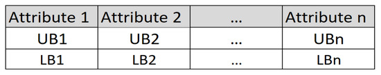
Figure 1.
QM_VMO representation of the nodes.
The node stores the intervals of each of the numerical attributes of the rule, as represented by Figure 2; it is important to mention that the node is a structure of the VMO algorithm itself.
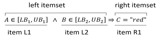
Figure 2.
Rule example.
4.4. Optimization Problem
Although the problem can be solved with a discrete optimization approach, we carry out a continuous optimization procedure. Considering the evaluation function, we determine as variables both the lower and upper limits of the intervals of each attribute of the rule.
Equation (16) defines the fitness function in more detail, and variables for m attributes of the rule are taken for optimization by means of the proposed method.
Association rules formed only by numerical attributes are processed directly by the numerical optimization method. Categorical attributes within the rule require preprocessing to generate new rule schemas based on each class.
4.5. Basic Definitions of the Proposal
QM_VMO (Quantitative Miner with the VMO algorithm) is our proposal for quantitative association rule mining based on the VMO algorithm. Basic definitions about some elements that are part of the procedures are introduced below. For this, a dataset with m numeric variables is considered, a rule scheme is defined, and a population of p individuals is generated.
- −
- : This value is calculated from the division between the range of the new interval and the range of the initial interval of the numerical attribute a.
- −
- Node: Let be a representation of p nodes that are part of a population; in QM_VMO, each node organizes the definition of a rule and is composed of one m-dimensional vector, the dimensions of the vector constitute each of the attributes that are part of the rule scheme, and the i-th node is defined in the following expression: , where are the lower bound and upper bound of the k-th attribute.
- −
- Population: In this technique, population refers to the set of p individuals that are part of a conglomerate, and is represented as follows: .
- −
- Mesh: in the studied context, the mesh is the set of nodes that are linked to exchange information and provide decision criteria in order to achieve an objective (objective function). The mesh is not a static structure. It is variable in time and can be represented in the following expression: ; this is the mesh defined at the t-th moment (iteration). The Mesh used by the QM_VMO algorithm ranges in size between and , and when using the expansion and contraction operators.
- −
- Initial mesh size: refers to the size of the population defined in the problem and is the number of nodes with which the mesh is initialized .
- −
- Final mesh size: refers to the maximum size that the mesh can reach in its expansion process; it is the number of nodes that the mesh has in a given iteration t—.
- −
- Neighborhood: is the neighborhood of that is defined by its k closest neighbors (determined with the Euclidean distance calculation).
4.6. The Proposed Approach for QM_VMO
The procedures and techniques covered by this research can be summarized in three levels of abstraction: (i) the definition of a rule template, (ii) the generation of the rule population, and (iii) the optimization of the intervals in the numerical attributes of the rule. The activation of the first level requires user intervention and access to the dataset. Then, the definition of a rule template can be processed. At the last level, the procedures deliver the most optimal rule or set of rules as a product.
The definition of a template is established by the user. The user configures the attributes of both the antecedent and the consequent. Using this matrix, it is possible to customize the possible combinations of attributes; this procedure is more specifically detailed in the subsection about the rule scheme.
The estimation of the amplitude is fundamental in reaching the diversity of the population. Equation (17) is used in the procedure to achieve the mentioned goal.
where , n is the size of the population, and N is the number of values in the domain of the attribute. The lower and upper thresholds of the ranges are defined as follows:
4.7. Achievement of the Rule Population
Starting from the general rule scheme defined by the user, we developed a procedure for obtaining a list of rule templates derived from the combinations of the attributes while respecting the scheme’s structure. The number of templates in the list is defined by Equation (18), where m is a parameter that establishes the maximum number of desired numerical attributes and n is the available quantity in the rule.
The size of the population is a parameter that can be customized by the user. The manipulation of this value allows one to find an appropriate fit. The individuals of the population defined before the general process are called the initial population, and they are obtained from the rule scheme (line 1 in Algorithm 2). It is important to generate populations of a very good quality. For this, diversity and breadth are two criteria that are considered, and they lead to the use of procedures based on random distributions and the introduction of control variables.
where , n is the number of attributes, , and m is the number of classes. So, for the achievement of a rule population from a scheme defined by Equation (19), with and a value of in the class, we have:
, where and n is the population size.
In an entire numeric scheme, a combinatorial explosion controlled by the number of numerical attributes that make up both the LHS and RHS of the rule takes place, and several templates are generated by this process. Equation (20) shows a general way to obtain each individual in the population, where and are the numbers of attributes in the LHS and RHS, respectively.
| Algorithm 2 QM_VMO algorithm. |
| Require: C,k,rTest |
| Ensure: best_node |
| 1: Generation of the rule population with Equations (17), (19) and (20) |
| 2: repeat |
| 3: foreach: do |
| 4: Find the closest k nodes using the Euclidean distance with Equation (2) |
| 5: Select the best local node |
| 6: if is better than then |
| 7: Calculate near factor between and with Equation (1) |
| 8: |
| 9: newRule = GetNewRule(n fValues) |
| 10: nnew = nodeRule(newRule, n fValues) |
| 11: foreach: do |
| 12: Calculate near factor between and and Equation (1) |
| 13: |
| 14: |
| 15: |
| 16: |
| 17: |
| 18: |
| 19: Fill nodes in the total mesh from |
| 20: Sort the nodes by the fitness quality in the total mesh |
| 21: Apply the clearing operator |
| 22: Build the mesh for the next iteration in an elitist way |
| 23: until C iterations |
| 24: best_node is obtained from the mesh (initial index) |
| 25: return best_node |
Notable changes in Algorithm 2 with respect to Algorithm 1 occur in the definition of the node for an optimization structure at the intervals of the numerical attributes that make up the rule. The new values for the intervals are updated in the rule schema, and a new rule is attained.
5. Results and Discussion
This study resulted in a version of the VMO algorithm used to solve the quantitative association rule mining problem. We called it QM_VMO. We conducted several experiments to evaluate the performance of QM_VMO, and all of the experiments were carried out on a computer with an Intel core I7 processor, 8 GB of RAM, and the Windows 10 operating system. To implement the algorithm, we used the Netbeans IDE 8.2 environment with JDK 1.8, while for the experimental analysis, R project v3.6 was used.
5.1. Preliminaries for the Experiments
Population meta-heuristics and all evolutionary algorithms require preliminary experimentation to obtain a good configuration of their parameters. We evaluated the sensitivity of some parameters, such as the size of the population and the number of evaluations. The tests were developed with three real databases from UCI Repositories and five synthetic ones.
We prepared five synthetic datasets, which are specified in Table 2; all used the same rule schema: between two and four numerical attributes on the condition side and one class attribute in the conclusion.
Table 2.
Summary of the experimental datasets.
To configure the experiment, we used the rule schemes defined in Table 3, from which we could generate rules of two to four numerical attributes. In the synthetic datasets, we used a single defined rule scheme of two to four numerical attributes in the LHS and a class in the RHS.
Table 3.
Experimental rule templates.
We inserted the experimental configuration into the code of the algorithm, so the number of iterations was defined in the vector = (100, 200, 500, 1000, 5000, and 10,000). QM_VMO required two parameters in order to set the population size: P (initial mesh size) and T (mesh expansion size); P = (8, 12, 24, 50 and 100) in all cases, the total expansion size used for this study was , and the number of closest neighbors was .
Table 4 shows the ordering with the fit function achieved by the algorithm in each of the configurations; thus, the population was in the rows. In contrast, the columns show the iterations tested. We proceeded with Equation (21) to obtain the values of column “R”; the results correspond to a statistical measure of variation and are interpreted according to an ascending order (lower indicates better quality).
Table 4.
Ranking of the sizes of populations with iterations.
In general, performance can be affected by the number of rows present in the database. To address this, we analyzed the behavior of our algorithm based on the size of the database. To do this, we will followed the same ordering structure as in the previous test, but this time, instead of iterations, we varied the dataset. We set the iterations to six hundred.
In Table 5, the minimum R is located in row 3, which corresponds to a population size of 24, thus supporting our chosen population. denotes the rankings assigned in different iterations, and is the ranking obtained in each dataset.
Table 5.
Ranking of the sizes of populations with rows of datasets.
Equation (21) is a utility measure based on the ordering of the evaluation function of the algorithm, where denotes the order assigned for each element of X, and STDEV(Xj) is the standard deviation for each evaluated population measure .
5.2. QM_VMO Performance Evaluation
We compared QM_VMO with the genetic version of QUANTMINER and three evolutionary algorithms from the literature: GAR [43], GENAR [50], and MODENAR [51]. The experimentation was carried out in the R project environment with the RKEEL version 1.3.1 library, which includes the last three algorithms mentioned. The tests were performed with nine databases, as described in Table 6. The algorithms’ parameters were configured according to the specifications from the literature, and QM_VMO used the values found by our analysis.
Table 6.
Datasets’ properties.
In Table 7, we show the initial configurations for the cited algorithms. The minimum support and confidence values in the case of the first two algorithms in the list were established at ten percent and sixty percent, respectively; for the others, they were adjusted according to need.
Table 7.
Setup of the algorithms for comparison.
In general, the comparison between algorithms with totally similar properties was not very achievable when referencing those existing in the literature. The configuration structure and requirements of our QM_VMO algorithm could be said to be very similar to those of QUANTMINER, and both required a rule scheme to start the process.
This specification allowed the user to obtain the desired rules more quickly. However, it could only explore rules generated by combining the attributes defined in the schema. The additional techniques that are cited do not define a rule template. They explore the entire set of a dataset’s attributes, thus allowing greater diversity to be achieved, but with the risk of converging on less understandable rules.
Figure 3 shows the average values of the support measure achieved for each dataset. Figure 4 presents the measure of confidence. With respect to the first two algorithms, the advantage obtained by our technique is more notable than that of QUANTMINER.
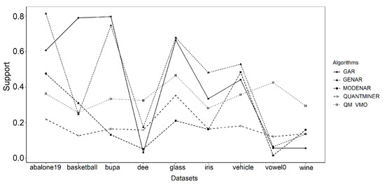
Figure 3.
Support measures for each dataset.
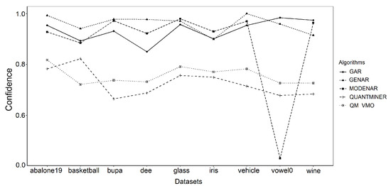
Figure 4.
Confidence measures for each dataset.
High coverage values for rule support are very significant when frequent patterns are found for qualitative variables. On the contrary, for quantitative attributes, they constitute a disadvantage in the quality of the rule. In fact, the average width of the interval is a criterion that was considered in the objective function that we used for our technique.
Another criterion of interest is the number of rules. However, the configuration of the parameters can condition the number of visible rules when the amount generated is too extensive. In general, the most representative rules are shown in order of the metric of interest.
Table 8 shows average values obtained in each of the metrics. Rules of all dimensions are considered to calculate the average number. However, there is a greater concentration on rules of 2, 3 and 4 attributes for all algorithms. Comparing QARMVMO and QUANTMINER is more precise due to their similarity in both configuration parameters and method. Other algorithms focus their optimization on a single population of rules (without defining schemes); due to that, their times are better, but they reduce diversity.
Table 8.
Main measures achieved by the algorithms.
Figure 5 shows the average values of the number of rules extracted by each algorithm, and these are distributed for rules composed of two, three, and four numerical attributes. The algorithms that exceeded this amount were not counted, although they were considered in the global rule count.
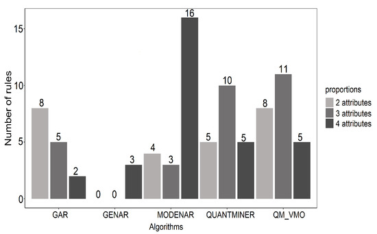
Figure 5.
Number of rules for each algorithm.
5.3. Synthetic Datasets
Additionally, to evaluate the sensitivity and performance of QM_VMO, we proceeded to generate synthetic datasets. For this, we evaluated some software alternatives, one of which was datasetgenerator. In the web version, this presented limitations in the customization of attributes and other parameters. The sequence database generator of the SPMF2 software and seq_data_generator3 modules were also evaluated, as they were more oriented toward transactional databases. Finally, we developed our script with R project to customize the experimentation requirements.
The simulated datasets were composed of five attributes that were created randomly with a uniform distribution. One of the attributes was categorical, and the others were continuous numeric variables, as described in Table 9. To give some coherence to the data, we assumed that our data were used to classify a segment of beneficiaries of a solidarity bond, so the class variable was defined under the categories of very_apt, apt, and no_apt and for the numeric variables of appraisal_house, income_familiar, spending_familiar, saving_banks, and age.
Table 9.
Description of the attributes in the synthetic datasets.
Figure 6 shows the optimization time as a function of the number of records (defined in thousands). Additionally, the number of functional attributes in the rule is considered. Here, n indicates the number of numerical attributes in the rule schema. Thus, for a given n, the execution time displayed here is the average time of several rules that have n numerical attributes.
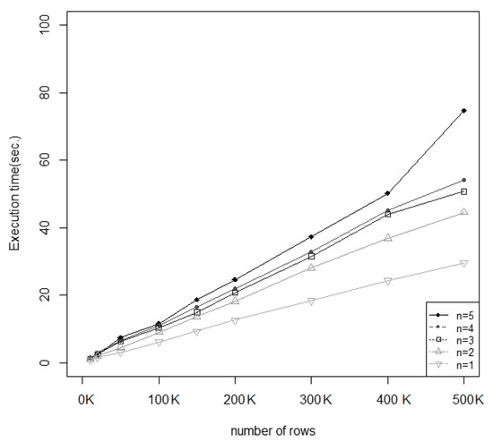
Figure 6.
Optimization time according to the number of rows.
6. Conclusions
In this work, we developed QM_VMO, which is an implementation based on the VMO algorithm, in order to solve the problem of the extraction of numerical association rules. To achieve this adaptation, we represented the definition of association rules in the node structure. The dimension of the problem is given by the number of numerical attributes involved, and these are optimized with functions of the VMO algorithm whose operators were adapted to work with this approach. Our technique was tested on real datasets available in the UCI Repositories, as well as on machine learning and synthetic datasets. In addition, four genetic algorithms were added; one of them had highly similar characteristics and the others were developed for the same objective. The results showed that QM_VMO presented higher-quality measures than those of the genetic version of QUANTMINER and reflected less sensitivity to the variations in the datasets. In addition, the generation of rules with greater comprehensibility was evident when the number of attributes that intervened in the rule was lower. The definition of the rule scheme by the user allows the customization of the desired solutions and reduces the search space, unlike in the other algorithms mentioned. The impact of the number of numerical attributes within the rule on the execution time is remarkable. However, this can be reduced with very well-specified rule schemes to thus avoid the combinatorial explosion.
7. Future Work
This research forms a basis for future scalable versions of the QM_VMO algorithm. Other approaches are possible in terms of both programming and the targeted varieties of data types. The field of big data requires emerging techniques for dealing with the concentration of trends of massive amounts of data.QM_VMO can be evaluated in that context and can be part of the new trends in data mining.
Author Contributions
Problematization, I.F.J.; Algorithm, I.F.J.; Writing—original draft preparation, I.F.J.; Writing—review and editing, J.G. and A.R. All authors have read and agreed to the published version of the manuscript.
Funding
This research received no external funding.
Institutional Review Board Statement
Not applicable.
Informed Consent Statement
Not applicable.
Data Availability Statement
Available in UCI Machine Learning Repository http://archive.ics.uci.edu/ml (accessed on 21 April 2021).
Conflicts of Interest
The authors declare no conflict of interest.
References
- Batrinca, B.; Treleaven, P.C. Social media analytics: A survey of techniques, tools and platforms. AI Soc. 2014, 30, 89–116. [Google Scholar] [CrossRef]
- Fayyad, U.; Piatetsky-Shapiro, G.; Smyth, P. From data mining to knowledge discovery in databases. AI Mag. 1996, 17, 37–54. [Google Scholar] [CrossRef]
- Linoff, G.S.; Berry, M.J.A. Market Basket Analysis and Association Rules, 3rd ed.; John Wiley & Sons: Indianapolis, IN, USA, 2011; Chapter 15; pp. 535–550. [Google Scholar]
- Lord, W.; Wiggins, D. Medical Decision Support Systems. In Advances in Health Care Technology Care Shaping the Future of Medical; Springer: Dordrecht, The Netherlands, 2006; Volume 6, pp. 403–419. [Google Scholar]
- Huang, Y.; McCullagh, P.; Black, N.; Harper, R. Evaluation of Outcome Prediction for a Clinical Diabetes Database. In Proceedings of the Knowledge Exploration in Life Science Informatics: International Symposium KELSI 2004, Milan, Italy, 25–26 November 2004; López, J.A., Benfenati, E., Dubitzky, W., Eds.; Springer: Berlin/Heidelberg, Germany, 2004; pp. 181–190. [Google Scholar]
- Mashiloane, L. Using Association Rule Mining to Find the Effect of Course Selection on Academic Performance in Computer Science I. In Proceedings of the Mining Intelligence and Knowledge Exploration: Second International Conference, MIKE 2014, Cork, Ireland, 10–12 December 2014; Springer International Publishing: Cham, Switzerland, 2014; pp. 323–332. [Google Scholar]
- Adhikary, D.; Roy, S. Trends in quantitative association rule mining techniques. In Proceedings of the 2015 IEEE 2nd International Conference on Recent Trends in Information Systems (ReTIS), Kolkata, India, 9–11 July 2015; pp. 126–131. [Google Scholar] [CrossRef]
- Camargo, H.; Silva, M. Dos caminos en la búsqueda de patrones por medio de Minería de Datos: SEMMA y CRISP. Rev. Tecnol. J. Technol. 2010, 9, 11–18. [Google Scholar]
- Liu, B.; Hsu, W.; Ma, Y. Integrating Classification and Association Rule Mining. In Proceedings of the Fourth International Conference on Knowledge Discovery and Data Mining, KDD’98, New York, NY, USA, 27–31 August 1998; AAAI Press: New York, NY, USA, 1998; pp. 80–86. [Google Scholar]
- Mattiev, J.; Kavsek, B. Coverage-Based Classification Using Association Rule Mining. Appl. Sci. 2020, 10, 7013. [Google Scholar] [CrossRef]
- Srikant, R.; Agrawal, R. Mining quantitative association rules in large relational tables. In Proceedings of the ACM Sigmod Record, Montreal, QC, Canada, 4–6 June 1996; ACM: New York, NY, USA, 1996; pp. 1–12. [Google Scholar]
- Ulrich, R.; Richter, L.; Kramer, S.; Universit, T. Quantitative Association Rules Based on Half-Spaces: An Optimization Approach. In Proceedings of the 2004 Fourth IEEE International Conference on Data Mining, ICDM’04, Brighton, UK, 1–4 November 2004; IEEE: Brington, UK, 2004; pp. 507–510. [Google Scholar]
- Miller, R.J.; Yang, Y. Association Rules over Interval Data. In Proceedings of the 1997 ACM SIGMOD International Conference on Management of Data, Tucson, AZ, USA, 11–15 May 1997; pp. 452–461. [Google Scholar]
- Chang, J.R.; Chen, Y.S.; Lin, C.K.; Cheng, M.F. Advanced Data Mining of SSD Quality Based on FP-Growth Data Analysis. Appl. Sci. 2021, 11, 1715. [Google Scholar] [CrossRef]
- Ou-Yang, C.; Wulandari, C.P.; Iqbal, M.; Wang, H.C.; Chen, C. Extracting Production Rules for Cerebrovascular Examination Dataset through Mining of Non-Anomalous Association Rules. Appl. Sci. 2019, 9, 4962. [Google Scholar] [CrossRef]
- Puris, A.; Bello, R.; Molina, D.; Herrera, F. Variable mesh optimization for continuous optimization problems. Soft Comput. 2012, 16, 511–525. [Google Scholar] [CrossRef]
- Salleb-Aouissi, A.; Vrain, C.; Nortet, C. QuantMiner: A Genetic Algorithm for Mining Quantitative Association Rules. In Proceedings of the 20th International Joint Conference on Artifical Intelligence, IJCAI’07, Hyderabad, India, 6–12 January 2007; Morgan Kaufmann Publishers Inc.: San Francisco, CA, USA, 2007; pp. 1035–1040. [Google Scholar]
- Salleb-aouissi, A. QuantMiner for Mining Quantitative Association Rules. J. Mach. Learn. Res. 2013, 14, 3153–3157. [Google Scholar]
- Panda, S.; Padhy, N.P. Comparison of particle swarm optimization and genetic algorithm for FACTS-based controller design. Appl. Soft Comput. 2008, 8, 1418–1427. [Google Scholar] [CrossRef]
- Putha, R.; Quadrifoglio, L.; Zechman, E. Comparing Ant Colony Optimization and Genetic Algorithm Approaches for Solving Traffic Signal Coordination under Oversaturation Conditions. Comput.-Aided Civ. Infrastruct. Eng. 2012, 27, 14–28. [Google Scholar] [CrossRef]
- Molina, D.; Puris, A.; Bello, R.; Herrera, F. Variable Mesh Optimization for the 2013 CEC Special Session Niching Methods for Multimodal Optimization. In Proceedings of the 2013 IEEE Congress on Evolutionary Computation, Cancun, Mexico, 20–23 June 2013; pp. 87–94. [Google Scholar] [CrossRef]
- Agrawal, R.; Imielinski, T.; Swami, A. Mining association rules between sets of items in large databases. ACM Sigmod Rec. 1993, 22, 207–216. [Google Scholar] [CrossRef]
- Agrawal, R.; Srikant, R. Fast algorithms for mining association rules. In Proceedings of the VLDB ’94: The 20th International Conference on Very Large Data Bases, Santiago, Chile, 12–15 September 1994; Bocca, J., Jarke, M., Zaniolo, C., Eds.; Morgan Kaufmann Publishers Inc.: San Francisco, CA, USA, 1994; pp. 487–499. [Google Scholar] [CrossRef]
- Chan, K.C.C.; Au, W.H. An effective algorithm for mining interesting quantitative association rules. In Proceedings of the 1997 ACM Symposium on Applied Computing—SAC ’97, San Jose, CA, USA, 28 February–1 March 1997; pp. 88–90. [Google Scholar] [CrossRef]
- Born, S.; Schmidt-Thieme, L. Optimal Discretization of Quantitative Attributes for Association Rules. In Classification, Clustering, and Data Mining Applications; Banks, D., McMorris, F.R., Arabie, P., Gaul, W., Eds.; Springer: Berlin/Heidelberg, Germany, 2004; pp. 287–296. [Google Scholar] [CrossRef]
- Moreno, M.N.; Segrera, S.; López, V.F.; Polo, M.J. A Method for Mining Quantitative Association Rules. In Proceedings of the 6th WSEAS International Conference on Simulation, Modelling and Optimization, SMO’06, Lisbon, Portugal, 22–24 September 2006; World Scientific and Engineering Academy and Society (WSEAS): Stevens Point, WI, USA, 2006; pp. 173–178. [Google Scholar]
- Song, C.; Ge, T. Discovering and Managing Quantitative Association Rules. In Proceedings of the 22nd ACM International Conference on Information & Knowledge Management, CIKM ’13, San Francisco, CA, USA, 27 October 2013–1 November 2013; Association for Computing Machinery: New York, NY, USA, 2013; pp. 2429–2434. [Google Scholar] [CrossRef]
- Adhikary, D.; Roy, S. A new equivalence class based approach for discretizing quantitative data using Point Shift Mechanism. In Proceedings of the 2015 International Symposium on Advanced Computing and Communication (ISACC), Silchar, India, 14–15 September 2015; IEEE: Silchar, India, 2015; pp. 174–180. [Google Scholar] [CrossRef]
- Aumann, Y.; Lindell, Y. A statistical theory for quantitative association rules. J. Intell. Inf. Syst. 2003, 20, 255–283. [Google Scholar] [CrossRef]
- Kang, G.M.; Moon, Y.S.; Choi, H.Y.; Kim, J. Bipartition techniques for quantitative attributes in association rule mining. In Proceedings of the IEEE Region 10 Annual International Conference, Proceedings/TENCON, Singapore, 23–26 January 2009; pp. 1–6. [Google Scholar] [CrossRef]
- Chien, B.C.; Lin, Z.L. An efficient clustering algorithm for mining fuzzy quantitative association rules. In Proceedings of the Joint 9th IFSA World Congress and 20th NAFIPS International Conference, Vancouver, BC, Canada, 25–28 July 2002; Volume 3, pp. 1306–1311. [Google Scholar] [CrossRef]
- Vannucci, M.; Colla, V. Meaningful discretization of continuous features for association rules mining by means of a SOM. In Proceedings of the ESANN2004 European Symposium on Artificial Neural Networks, Bruges, Belgium, 28–30 April 2004; pp. 489–494. [Google Scholar]
- Lian, W.; Cheung, D.W.; Yiu, S.M. An efficient algorithm for finding dense regions for mining quantitative association rules. Comput. Math. Appl. 2005, 50, 471–490. [Google Scholar] [CrossRef][Green Version]
- Yunkai, G.U.O.; Junrui, Y.; Yulei, H.; Guo, Y.; Yang, J.; Huang, Y. An Effective Algorithm for Mining Quantitative Association Rules Based on High Dimension Cluster. In Proceedings of the 2008 4th International Conference on Wireless Communications, Networking and Mobile Computing, Dalian, China, 12–14 October 2008; IEEE: Dalian, China, 2008; pp. 1–4. [Google Scholar] [CrossRef]
- Junrui, Y.; Zhang, F. An effective algorithm for mining quantitative associations based on subspace clustering. In Proceedings of the 2010 2nd International Conference on Networking and Digital Society (ICNDS), Wenzhou, China, 30–31 May 2010; Volume 1, pp. 175–178. [Google Scholar]
- Zhang, W. Mining fuzzy quantitative association rules. In Proceedings of the 11th International Conference on Tools with Artificial Intelligence, Chicago, IL, USA, 9–11 November 1999; pp. 99–102. [Google Scholar] [CrossRef]
- Gyenesei, A. Mining weighted association rules for fuzzy quantitative items. In European Conference on Principles of Data Mining and Knowledge Discovery; Springer: Berlin/Heidelberg, Germany, 2000; pp. 416–423. [Google Scholar]
- Yang, J.; Hu, X.; Fu, Y. Fuzzy Association Rules Mining Algorithm FMFFI Based on Bidirectional Search Technique. In Proceedings of the 2015 7th International Conference on Intelligent Human-Machine Systems and Cybernetics, Hangzhou, China, 26–27 August 2015; Volume 2, pp. 440–443. [Google Scholar] [CrossRef]
- Varol Altay, E.; Alatas, B. Intelligent optimization algorithms for the problem of mining numerical association rules. Phys. Stat. Mech. Appl. 2020, 540. [Google Scholar] [CrossRef]
- Feng, H.; Liao, R.; Liu, F.; Wang, Y.; Yu, Z.; Zhu, X. Optimization algorithm improvement of association rule mining based on particle swarm optimization. In Proceedings of the 2018 10th International Conference on Measuring Technology and Mechatronics Automation (ICMTMA), Changsha, China, 10–11 February 2018; pp. 524–529. [Google Scholar] [CrossRef]
- Cao, Y.; Zhang, H.; Li, W.; Zhou, M.; Zhang, Y.; Chaovalitwongse, W.A. Comprehensive Learning Particle Swarm Optimization Algorithm With Local Search for Multimodal Functions. IEEE Trans. Evol. Comput. 2019, 23, 718–731. [Google Scholar] [CrossRef]
- Wang, Y.; Gao, S.; Zhou, M.; Yu, Y. A multi-layered gravitational search algorithm for function optimization and real-world problems. IEEE/CAA J. Autom. Sin. 2021, 8, 94–109. [Google Scholar] [CrossRef]
- Mata, J.; Alvarez, J.J.L.; Riquelme, J.C.J. Discovering numeric association rules via evolutionary algorithm. In Advances in Knowledge Discovery and …; Chen, M.S., Yu, P.S., Liu, B., Eds.; Springer: Berlin/Heidelberg, Germany, 2002; pp. 40–51. [Google Scholar]
- Beiranvand, V.; Mobasher-Kashani, M.; Abu Bakar, A. Multi-objective PSO algorithm for mining numerical association rules without a priori discretization. Expert Syst. Appl. 2014, 41, 4259–4273. [Google Scholar] [CrossRef]
- Martín, D.; Rosete, A.; Alcalá-Fdez, J.; Herrera, F. A New Multiobjective Evolutionary Algorithm for Mining a Reduced Set of Interesting Positive and Negative Quantitative Association Rules. IEEE Trans. Evol. Comput. 2014, 18, 54–69. [Google Scholar] [CrossRef]
- Geng, L.; Hamilton, H.J. Interestingness measures for data mining. ACM Comput. Surv. 2006, 38, 1–32. [Google Scholar] [CrossRef]
- Martínez-Ballesteros, M.; Martínez-Álvarez, F.; Troncoso-Lora, A.; Riquelme Santos, J. Selecting the best measures to discover quantitative association rules. Neurocomputing 2014, 126, 3–14. [Google Scholar] [CrossRef]
- Berzal, F.; Cubero, J.C.; da Jiménez, A.; Berzal, F.; Cubero, J.C. Interestingness Measures for Association Rules. Intell. Data Anal. 2010, 17, 298–307. [Google Scholar] [CrossRef]
- Fukuda, T.; Morimoto, Y.; Morishita, S.; Tokuyama, T. Mining Optimized Association Rules for Numeric Attributes. J. Comput. Syst. Sci. 1999, 58, 1–12. [Google Scholar] [CrossRef]
- Mata, J.; Mata, J.; Alvarez, J.L.; Alvarez, J.L.; Riquelme, J.C.; Riquelme, J.C. An evolutionary algorithm to discover numeric association rules. In Proceedings of the 2002 ACM Symposium on Applied Computing—SAC , Madrid, Spain, 1–14 March 2002; p. 590. [Google Scholar] [CrossRef]
- Alatas, B.; Akin, E.; Karci, A. MODENAR: Multi-objective differential evolution algorithm for mining numeric association rules. Appl. Soft Comput. 2008, 8, 646–656. [Google Scholar] [CrossRef]
Publisher’s Note: MDPI stays neutral with regard to jurisdictional claims in published maps and institutional affiliations. |
© 2021 by the authors. Licensee MDPI, Basel, Switzerland. This article is an open access article distributed under the terms and conditions of the Creative Commons Attribution (CC BY) license (https://creativecommons.org/licenses/by/4.0/).