Abstract
Automatic glia reconstruction is essential for the dynamic analysis of microglia motility and morphology, notably so in research on neurodegenerative diseases. In this paper, we propose an automatic 3D tracing algorithm called C3VFC that uses vector field convolution to find the critical points along the centerline of an object and trace paths that traverse back to the soma of every cell in an image. The solution provides detection and labeling of multiple cells in an image over time, leading to multi-object reconstruction. The reconstruction results can be used to extract bioinformatics from temporal data in different settings. The C3VFC reconstruction results found up to a 53% improvement on the next best performing state-of-the-art tracing method. C3VFC achieved the highest accuracy scores, in relation to the baseline results, in four of the five different measures: Entire structure average, the average bi-directional entire structure average, the different structure average, and the percentage of different structures.
1. Introduction
The recent realization that the central nervous system (CNS) and the immune system are not two isolated systems, but rather connected systems, implies the relationship and interaction between neurons and immune cells in the CNS [1,2]. Researchers are attempting to understand the impact of microglia not only in development and homeostasis, but also their role in injury, diseases, and aging [3,4,5,6]. The morphological changes of microglia are directly associated with functional roles in normal and pathological central nervous systems. Microglia have processes, or branches, that extend from the soma, or cell body. In a healthy brain, the processes dynamically extend and retract to respond to changes and to surveil the environment [7,8,9,10,11,12]. However, in response to diseased settings, activated microglia transition from a highly ramified state to a less ramified, amoeboid state [13,14]. These changes suggest that microglia may be related to the progression of neurodegenerative diseases, such as Parkinson’s disease, multiple sclerosis, and Alzheimer’s disease. However, little is known about how the decrease in the activity and motility of a microglia’s processes affect the microglia’s ability to perform surveillance functions in the brain. This work meets a major need of the immunology and neuroscience communities; namely, it provides a toolbox of image-based bioinformatics for glia.
Quantifying morphological changes can lead to understanding the function and activation of microglia in different settings. The complex structure of the thin microglia processes and inhomogenous, noisy microscopy images make manual and automatic tracing challenging. Currently, most glia image analysis is done by hand, where scientists manually trace the processes. With high-throughput imaging, researchers may be able to reveal a quantitative model of morphological differences, but in such cases, manual analysis is infeasible. Existing studies have manually traced glial images or used heuristic image processing methods to measure process length, extension, and retraction over time [15,16,17,18,19]. However, manual tracing can be prone to human error and user-variability. Ramified microglia have fine processes that can intertwine which makes it difficult to distinguish between cells. Most tracings done for analysis was performed on 2D images where branches overlap or are occluded and lead to further loss of information and inaccurate analysis. Manual or semi-automated methods are time-consuming with high-throughput imaging and larger datasets. Common automatic image analysis approaches used for quantification depend on thresholding inhomogenous and noisy images which result in over-segmented reconstructions or an under-segmentation with missing branches. Some papers related to the reconstruction and analysis of microglia have provided significant contributions to the structural analysis of these cells, but they use thresholding techniques that are are not able to accurately capture the entire cell [19,20].
Our goal is to create an automatic tracing method that achieves consistent reconstructions of 3D images over time to obtain an accurate analysis of the image and video data. An accurate tracing of tubular cells yields the medial axis, or centerline, of the structure. In [21,22], the researchers developed an algorithm that automatically skeletonized and segmented 3D images of microglia. They were able to find the centerline of the processes using an active contour method and gradient vector field. However, the image was reconstructed one pixel or voxel at a time to counter the difficulties of open curve tracing. Other centerline tracing methods find and connect endpoints and critical points of an object [23]. Critical points indicate the key structural changes of an object and can be identified by analyzing the topology of vector fields. These critical points are located at some “saddle points” and “attracting points” along the vector field of an image, which can be determined from an eigenvalue analysis [23,24,25]. Finding these points can be computationally expensive and difficult with noisy real images of limited resolution. Other methods find the local maxima on the object of interest to create a minimum spanning tree [26,27,28]. Some methods are motivated by the tubular structure of neurons and glia cells to initialize their method using vesselness enhancement [21,29,30,31]. The accuracy of the vessel enhancement relies on selecting the correct width of the tubular structure, given that the scale does not vary for a given object. In this paper, we demonstrate the automation of quantification of glial morphology and activity in different settings for 3D images and videos.
2. Background on Vector Field Convolution
Vector field convolution (VFC) was proposed as an external force field for an active contour method used in image segmentation. The basic idea was to compute vectors that pointed at image edges and then to diffuse such forces across the image via tensor convolution. The resultant VFC fields are robust to noise and to the initialization of an active contour [32]. The convolution-based approach was also used to reconstruct a skeleton for neuron images in [33] by acquiring a VFC medialness map, an enhanced medial-axis image, which they used to create a graph minimum spanning tree. However, these methods rely on finding the correct scale to accurately reconstruct the image, but result in disjointed segments due to intensity inhomogeneity and noisy images. The authors attempted to reconnect the disjointed segments using a graph-connectivity algorithm that was based on the orientation and distance of the segments from one another [34,35]. Attempting to reconnect disjointed segments in glia images based on orientation and distance result in incorrect connections due to the complexity of branches within one cell and between other intra-cell branches.
Our method, C3VFC, utilizes VFC in an open curve tracing methodology to find the critical points and centerline, or skeleton, of multiple objects within 3D videos. This technique, based on VFC, is an enabling image analysis technology that paves the way for reliable microglia reconstruction.
In [32], the open curve is a parametric active contour model that is deformed toward edges in the image, controlled by the external and internal energy. The external force guides the active contour towards the edges using image features. The internal force is guided by the qualities of the contour, such as smoothness or tautness. The contour is represented as a set of contour points and the initial points are parameterized between . The initialized snake contour is evolved by minimizing an energy functional:
where and are the parameters for controlling smoothness and bending of the contour, respectively. In [32], the authors defined the external energy, , with the vector field convolution force, .
An active contour model for open splines needs to be constrained so that the points along the contour do not drag into itself and vanish. For every iteration, the curve is updated where the set of contour points may shrink or grow. For a vector field that points towards the medial axis of an object, the intensity inhomogeneity within the object may cause parts of the medial axis to have a greater pull on the vector field. However, constraining the end points of a contour for a non-continuous structure, such as a microglia, typically involves splitting an object into multiple parameterized contours, or branches. In [21], the authors constrained the open curve snake by evolving the contour one point, or seed, at a time, controlling the elasticity and connection of all seed points to each other, which, if used in larger data sets, could be computationally expensive. Other open curve snake methods improved on this work by automatically initializing fewer, more accurate, seed points to evolve the seeds toward each other following the gradient vector field [36,37,38]. These methods largely rely on finding seeds that are already initialized on the centerline.
3. Materials and Methods
C3VFC is our automated tracing system that computes the skeleton of objects in a 3D image over sequential time frames, which facilitates accurate biological analysis and quantification via the extraction of bioinformatics. The method is described in Figure 1 and in Algorithm 1. The number of objects in the image are determined by automatically detecting the soma, or the cell body, and its corresponding critical points, so that each object can be individually traced in parallel. Critical points are detected for each object by evolving seed points, or the initialized points, that are constrained by concentric circles around each soma. The final temporal skeletons are extracted via a fast marching method from the critical points and a centerline map. The temporal reconstructions can be used for accurate biological analysis. In this paper, we compare our reconstruction results from C3VFC and from state-of-the-art methods with those derived from the baseline standard manual tracing.
| Algorithm 1:Procedure for C3VFC for tracing medial axis of glia |
 |
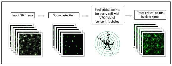
Figure 1.
C3VFC methodology.
3.1. Imaging Acquisition and Fluorescence Technique
The multi-cellular dataset consists of 3D images of microglia from living mice using in vivo multiphoton microscopy, see supplementary materials SI2–SI4. Heterozygous GFP reporter mice expressing GFP under control of the fractalkine receptor promoter () were used for the imaging studies. Wild-type C57/B6 mice were crossed with mice from Jackson labs (stock no. 005582) to generate for these experiments to visualize microglia. For in vivo imaging, mice were implanted with a chronic cranial window as previously described [39]. Briefly, during surgery, mice were anesthetized with isoflurane (5% for induction; 1–2% for maintenance) and placed on a heating pad. Using a dental drill, a circular craniotomy of >3 mm diameter was drilled at 2 mm posterior and 1.5 mm lateral to bregma, the craniotomy center was around the limb/trunk region of the somatosensory cortex. A 70% ethanol-sterilized 3-mm glass coverslip was placed inside the craniotomy. A light-curing dental cement (Tetric EvoFlow) was applied and cured with a Kerr Demi Ultra LED Curing Light (DentalHealth Products). iBond Total Etch glue (Heraeus) was applied to the rest of the skull, except for the region with the window. This was also cured with the LED light. The light-curing dental glue was used to attach a custom-made head bar onto the other side of the skull from which the craniotomy was performed.
To label microglia in the mouse brain for the dataset in supplementary materials SI1, we used mice with an inducible Cre recombinase under the control of the CX3CR1 promoter crossed to the Ai6 fluorescent reporter mouse (Jackson Laboratories, Bar Harbor, ME) to generate X Ai6ZsGreen [40,41]. At post-natal day (P23) 23 mice were given 10 uL/g body weight of a 20 mg/mL Tamoxifen (Sigma) solution in corn oil to induce recombination of the floxed stop codon leading to ZsGreen expression in microglia.
All procedures adhered to guidelines of the Institutional Animal Care and Use Committee (ACUC) at the University of Virginia. Microglia of adult mice (7–10 weeks old) were imaged using a Leica TCS SP8 multiphoton microscopy system equipped with a Coherent Chameleon Ti:Sapphire laser and a 25 × 0.95 NA immersion lens.
3.2. Dataset
The multi-cellular 3D movies of microglia were imaged over 16 min taken at one minute intervals, containing multiple microglia per field of view. The 3D images were 1024 × 1024 × 61 pixels where the x-y frame was 295 m × 295 m. For each image, there were 61 z-stacks acquired and the z-stack depth was taken in 1-m intervals. There are about 37 different cells in the multi-cellular video dataset, see supplmentary materials SI2–SI4. SI1–SI3 are microglia in naive mice, or mice that have not been previously subjected to experiments. SI4 is a video of the same microglia in SI3 that has been subjected to laser burn-induced injury. The processing of 3D images is very difficult because the varying intensity throughout the cell and non-structural noise along the z-stack make the actual cell signals hard to be visualized. To increase the intensity throughout the cell regions and the contrast of the images for further processing, histogram equalization was applied, although some noise in the background may be increased too. The images were taken in naive mice and mice with laser burn-induced injuries that would vary the movement and morphology between the videos.
3.3. C3VFC: Tracing Glia in 3D Temporal Images
A 3D vector field is computed using vector field convolution [32] on the original image, , to find the centerline that lies on the maximum intensity of an object, which is also the centerline of the object. A vector field kernel, , is convolved with so that the vector field points towards the centerline. The vector field is defined as:
where ⊛ is defined as linear convolution. The vector kernel is defined as:
where is the magnitude of the vector kernel and is the unit vector pointing towards the kernel origin at (0,0,0):
where is the distance from the origin. The origin of the kernel, (0, 0, 0), is considered the location of the features of interest (FOI), so a particle that is placed in that field is able to move towards the FOI, which in this case is the centerline. Thus, the further away the particles are from the origin, the smaller the influence of the FOI, and the magnitude of the vector field kernel is a decreasing function of distance from the origin:
where is a parameter that controls the influence of the FOI, and should be changed according to the signal-to-noise ratio, and is a small positive constant that avoids dividing by zero.
The VFC external force is calculated by finding the convolution between the vector field kernel and the intensity image . For a 3D image, the VFC force field would be comprised by a three directional vector field in which the vectors point towards the centerline of a 3D object.
Figure 2 depicts the VFC field on a microglia image. A 3D image of microglia is convolved with the vector kernel in Equation (3) to produce a VFC field that points to the centerline of the objects. Although not shown in the figure, the 3D vector field points to the center line in the x-y-z direction. The vector’s magnitude and direction relies on the intensity of the image and the parameters of the kernel. In a real image, the noise pulls the vectors in the background but the large capture range of the kernel pull the vectors towards the higher intensity of the foreground object, or the centerline.
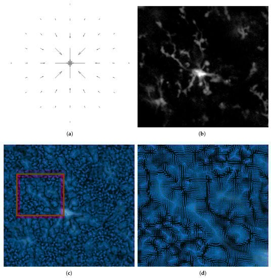
Figure 2.
The VFC field of the intensity image. (a) The kernel is convolved with (b) the original image (slice 8 of 16 in the z-stack is shown) to produce VFC field. (c) The VFC field. (d) Zoomed-in VFC field of the red box in (c).
In a real image, there is varying intensity throughout the object, where some intensities may be stronger in thicker parts of the object. Thus, there are non-zero vectors on the centerline that would move free particles towards a converging point, where ideally we would like the seeds to stop in the centerline. Our workflow solves these challenges by detecting and labeling the cells, using the VFC field to find critical points in the cells, and tracing them back to the soma.
3.3.1. Initialization
The goal of C3VFC is to trace glia in single- and multi-cellular 3D images, I, over consecutive time frames. Biological images acquired through microscopy imaging have low signal-to-noise ratio (SNR) and background noise so we want to ensure that the points are evolved within the region of interest. The Hessian matrix of partial derivatives describes the local curvature of an image [42]. The visualization of the initialization is depicted in Figure 3. The eigenvector of the Hessian describes the concavity at points in the image. The attained eigenvectors can be sorted via the absolute value of their eigenvalues. The most negative eigenvalue, , describes the highest curvature. The voxels at which is set to zero. The remaining voxels are the foreground pixel in . This will be the initial seed points that will be evolved towards the centerline of the parts of the object via our open curve tracing method.
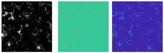
Figure 3.
The initial seed points are determined using curvature analysis. The original image (left) is analyzed with a curvature analysis (middle) to find the foreground image (right).
3.4. Soma Detection and Labeling Cells over Time
In glia cells, the processes extend and retract from the soma. The cell bodies can be utilized to determine the number of cells and its respective processes in an image. The soma can be distinguished by its overpowering intensity and volume compared to the fine processes. We automatically detect and reconstruct the soma from the input image via the blob flow field (BFF) method [31]. In this approach, eigenvectors attained from the Hessian matrix of a Gaussian-smoothed image are ordered by the increasing magnitude of the eigenvalues, [43]. BFF enhances blob-like structures by finding structures in the image with high values of in the three orthonormal directions. Once the blobs are detected, the edge-based active contour algorithm moves the contour towards the soma boundary.
The soma detection method find s number of soma in the given input image, which is used to label detected soma over consecutive time frames. As seen in Figure 4, it is difficult to determine the soma shape and separate touching cells in 2D images, which are z-stack projections of the 3D image. Some cell processes and soma may be overlapping or occluded in the z-stack of a 2D view. However, a tilted view of the 3D image reveals the actual number of cells in a given region. Knowing the correct number of cells and soma shape allows our algorithm to trace the processes back to the appropriate soma. Figure 4c shows some processes that belong to cells where the soma is not in the field of view and only portions of a cell are captured. This inevitable issue presents a challenge for constructing the tracing methodology. It can be argued that only cells that are fully in the region of interest need to be segmented for quantification and analysis. C3VFC uses the detected soma to find and label the corresponding soma over consecutive time frames. Consequently, corresponding glia are automatically labeled over time with respect to their corresponding soma.
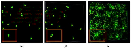
Figure 4.
Soma detection: (a) 2D view, (b) 3D view, and (c) 3D tracing of each cell. The red box in the images indicate the region of interest where soma overlap and would be difficult to distinguish in the top 2D projection of the 3D image.
3.5. Tracing Multiple Objects in a 3D Image
The objects in the images, or cells, are non-continuous points that are connected at the soma. These points could be parameterized in segments, as with the methods mentioned in Section 2, or represented as free particles without an internal force, as in Equation (1). Since the seed points are non-continuous, the internal force of the active contour energy functional would not acquire the desired smoothing and bending constraints. Therefore, the energy functional would be dependent on the VFC field from Equation (2). The initial contour points for the image is which is represented by N discrete points . The update procedure is iterative:
where t is the iteration and is the step size,
and
The VFC field for the image contains vectors on the centerline that point to higher intensity values within the object of interest. Vectors along the centerline may cause points to vanish into each other instead of providing a continuous tracing. To resolve these open curve tracing issues, our method finds critical points throughout the object.
3.6. Concentric Circles, VFC, Critical Point Detection
The cells in the image are detected via soma detection and corresponding cells are labeled over consecutive time frames. Thus, all the processes can be traced back to its corresponding soma. As mentioned in Section 2, critical points are typically determined through an eigen value analysis of the image vector field and represent the structural changes along the object of interest. In C3VFC, the critical points are determined by using an active contour evolution using the vector field of concentric spheres around each glia. The concentric circles are placed around the soma of every detected cell, shown in Figure 5a. The concentric circles are:
where the coordinates represents the soma, is the radius of the soma, and is the distance between the concentric circles, and where M is the maximum number of concentric circles. The distance between concentric circles, , is a user-input parameter. The maximum number of concentric circles, M, is determined by the farthest initialized distance from the soma divided by . The vector kernel, from Equation (3), is convolved with the intersection of the concentric circles and the intensity image to find the vector field:
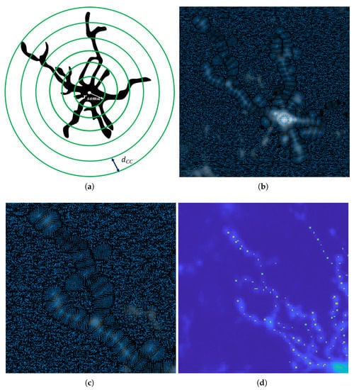
Figure 5.
The VFC fields to find critical points of an object. (a) Concentric circles are placed around every detected soma to find (b)the vector field of the intensity image on these circles (c) zoomed in (d) the critical points on the object of interest.
This force field constrains the evolution of seed points to the spheres to ensure that the critical points are constrained to the centerline on these areas, as shown in Figure 5c,d. Equation (10) is a important contribution in our method that uses the VFC field to find the critical points in an object that lie on the centerline. In this case, we only want to evolve the initial points that lie on the concentric spheres around the objects. The initial contour points is extracted from the initial foreground image explained in Section 3.3.1: that also intersect with concentric circles for a given soma, . Figure 5 shows that the vector field will carry the seeds to the critical point on the intersection of the branches and the concentric sphere, using Equation (6). The updated foreground vertices become the critical point list which is used to trace processes back to the soma of each microglia.
3.7. Tracing Cells Back to Soma
The critical points described in the previous section lie on the centerline of the processes. Each point from the critical point list is traced back to the soma detected in the first step of C3VFC. The critical points and the soma could be thought of respectively as the start and end points on a path. The path that reaches the endpoint in the least amount of time within an image domain is the geodesic path. The minimal path problem can be solved with the multi-stencil fast marching algorithm [44]. The time arrival map is initialized with the result of the initial foreground, , updated using the VFC field from Equation (2). These points do not form a continuous tracing of the glia but they lie on the centerline. The rest of the time arrival map is formed with the distance transform of the initialized seeds in Section 3.3.1. The fast marching algorithm computes the fastest path to get from one point to another.
For every object detected in the image, the critical points are a set of points on the centerline that will be traced back to the soma. We start with the farthest critical point from the soma to traverse through the path. After every iteration, we remove points that lie on the traced path from the critical point list. Then, the next point farthest from the soma is traced back to the soma until there are no more critical points in the set.
The output of our tracing workflow is a skeleton image that can be represented in the SWC file format (in this case, SWC is the concatenation of the last initials of the inventors of the format [45]). The SWC file is a standard format for biological images with tree structures and is widely used by neuroscientists. With the SWC format, each foreground-traced pixel of the connected cell is saved in the matrix format with seven fields: Index number, structure type, three x-y-z coordinates, radius, and parent connection node. Since our algorithm detects and reconstructs the soma, we have formatted the SWC file to save the entire soma as the root node for accuracy. Typically the soma, or root node, is indicated by just the first row of the SWC file which is indicated by as the parent connection node. Our SWC format saves all the soma voxels in the SWC file with a as the parent connection node. Any child node of a soma voxel will indicate the index number as their parent connection node.
4. Results
4.1. Performance Evaluation
We use datasets consisting of 3D images of microglia over a time of 16 min, as described in Section 3.2. We compare the temporal tracing results from C3VFC with results from state-of-the-art automatic skeleton reconstruction methods including improved all path pruning version 2 (APP2) [46], fast marching minimum spanning tree (FMST) [28], and minimum spanning tree (MST) [26]. APP2 is one of the fastest state-of-the-art methods for neuron tracing and has been used as the gold standard in some neuron reconstruction studies. APP2 is based on fast marching and hierarchical pruning and has proven that it can achieve complete reconstructions for images with uneven pixel intensities, fine branches, and irregular-sized cell bodies. We also compare our results with FMST and MST since both algorithms achieve higher or similar accuracy reconstruction scores than results from APP2 in numerous studies. MST uses local maxima to find points on the object of interest to create a minimum spanning tree to trace neurons. FMST is an advancement of the MST algorithm with the advantage of an over-segmentation and pruning method that is similar to that of APP2. The Vaa3D software was used to implement APP2, FMST, and MST. Vaa3D is short for 3D Visualization-Assisted Analysis software suite that is currently maintained and updated by HHMI—Janelia Research Campus and the Allen Institute for Brain Science [47,48,49,50]. For MST, the parameters for the window size were set to 10 or 15 depending on which value obtained a better result. The default settings for APP2 were used since they gave the best results. However, the output of the three comparison methods were insufficient for multi-cellular images. From Figure 6, we see that APP2 could not detect over 50% of cells in a given image. Meanwhile, FMST and MST could not separate cells in a multi-cellular image. Thus, for the performance evaluation comparisons, each individual cell had to be manually cropped before inputting the image into APP2, FMST, and MST. However, the entire multi-cellular image was input into C3VFC and the output was the reconstruction image and SWC file format for all detected cells that were labeled over consecutive time frames. The individual labeled glia were easily manipulated for comparison.
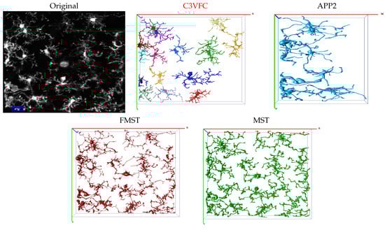
Figure 6.
Visual comparison of the multi-cellular reconstruction results using C3VFC (our method), APP2, FMST, and MST. Separated cells are distinguished by color for the result of every method.
The accuracy of all the automatic reconstruction results are found against a baseline manual result. The baseline manual result is attained using the Simple Neurite Tracer in the ImageJ software [51]. The software allows for a semi-manual tracing setting in which the user could slide through the z-stacks of a 3D image and connect points along the branch paths. We note that the baseline manual result may have user error due to background noise and intensity inhomogeneity throughout the object of interest and through human error of estimating the centerline, especially through the z-stack view. The branch complexity of the cell and the resolution of the confocal microscope make it difficult to distinguish the path of each branch and between cells that are in close proximity or touching. The 3D image captures a specific region of interest, so the soma of some branches may be occluded from the 3D image. Parts of some branches also extend outside the 3D image. These inevitable issues cause reconstruction error for both the automatic algorithms and the expert manual tracer.
Figure 7 shows the visual tracing results between the original image, the manual baseline, our result, and the result from the comparisons. Although C3VFC outputs the skeleton for all the cells in the entire image, individual cells are shown in the figure for a visual comparison against other methods. In our method, every cell is detected and labeled over time based off of the soma detection. This allows for a simple conversion from a 3D skeleton image to SWC files and the extraction of bioinformatics.
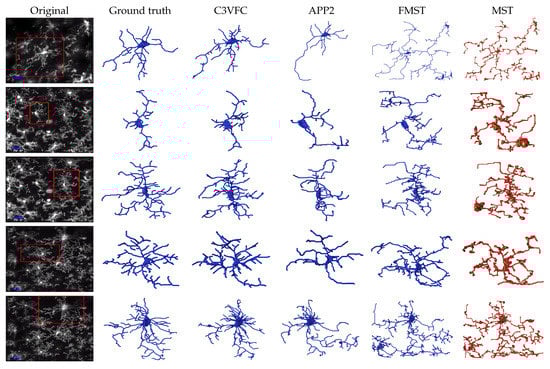
Figure 7.
Reconstruction results of 3D microglia images. The first column on the left is the original image with the region of interest boxed out on the left. The following columns show the 3D reconstruction in the SWC format.
There is disagreement in the research community regarding how to evaluate the accuracy of a skeleton reconstruction. Manually tracing an object is indeed subject to intra-user and inter-user variability, especially in 3D, but such manual measurements represent the best existing choice for a baseline of quality. We use five different distance measures to measure the error between the baseline and reconstruction results. We evaluate the performance of the reconstructions by measuring the average Euclidean distance between the reconstruction result and ground truth. We input the SWC format reconstructions into Vaa3d to measure the entire structure average from 1 to 2 (), ESA from 2 to 1 (), average bidirectional-ESA (ABESA), difference structure average (DSA), and percentage of different structure (PDS), which were introduced and defined in [47]. is a measure of the distance of a voxel from the ground truth to the closest voxel on the reconstruction result. is a measure of the distance of a voxel from the reconstruction result to the closest voxel on the ground truth. refers to the smallest spatial distance of a voxel between the reconstruction result to the closest voxel on the ground truth. refers to the average spatial distance for the voxels that are different between the reconstruction result and the ground truth result. is the percentage of the voxels that are different between the reconstruction result and the ground truth result. We use the default value of “2 voxels” in spatial distance to account for human error, because the authors in [47] experimentally proved that this default value gives sufficient visual difference to distinguish different results. Table 1 shows the average and standard deviation of these distances compared with the manual baseline result. A lower value for each of these distances signify a higher accuracy measure to the ground truth.

Table 1.
Performance evaluation of results. The five measures computes the distance of the baseline manually traced results to the results from the respective methods. A lower value signifies better performance for all distance measures. The values in bold signify the best scores for each measure.
From Table 1, C3VFC has a lower error in all of the measures compared to APP2, FMST, and MST. APP2 achieved the second-closest distance for four of the five measures: , , , and . FMST and MST have a low but higher values signifying that their reconstruction contained a larger amount of false positive branches. FMST and MST also had the largest PDS values which tells that these reconstructions were the most different to the baseline reconstruction. The visual testimonial can be seen in Figure 7 where FMST and MST capture erroneous branches and noise that do not belong to the cell of interest. APP2 showed the most competitive results for all scores but it seemed to have missed the shorter processes and may over-prune its segmentation results. It must be noted that APP2 did not perform well when the entire multicellular image was input into the algorithm, as shown in Figure 6. FMST and MST seemed to be an over-segmentation, which was posed as an advantage of their algorithms, but the pruning was insufficient for glial images. From Table 1, if we consider the mean distance measure with the standard deviation, C3VFC achieves the best performance in four of the five accuracy measures: , , , and . The mean distance measure with the standard deviation requires adding and subtracting the standard deviation from the mean to find the range of distance measures. C3VFC found up to a 53% improvement compared to APP2, FMST, and MST using the five accuracy measures ( and ). This percentage was attained by calculating the improvement of the worst distance measure for C3VFC over the next best distance measure in the comparison methods in Table 1. The worst accuracy measure for C3VFC was found by calculating the worst mean with the standard deviation of the measures. The worst performance for C3VFC would be for . This value is subtracted from the best performance measure for achieved by the comparison algorithms, which was attained by APP2, to then find the percentage of improvement.
The standard deviation in the measures for C3VFC could partially be attributed to the algorithm capturing parts of another cell, as shown in the temporal visualization in the video in the supplementary materials that is labeled SI1. Since our method takes in the entire image with multiple cells, the accuracy is attributed to detecting the correct number of somas and cells. However, the 3D images may capture some processes that have corresponding soma outside of the 3D image, thus these processes may not be traced or erroneously picked up by another cell. Additionally, our method attempts to prevent capture of erroneous branches with the vector field, but some branches are touching and make it difficult to separate even with the human expert’s eye. C3VFC intentionally does not trace branches with a corresponding soma not in the field of view, unless it is erroneously captured as stated previously. The purpose of the C3VFC algorithm is to trace temporal images for dynamic microglia analysis, and so, lone branches are considered to be background objects. C3VFC takes an average of 10 min to trace the each image, which is dependent on the number of branches that are traced back to the soma. The other algorithms, APP2, MST, and FMST, require about 20 s per image. However, we must note that C3VFC traced the entire multi-cellular image, while the other three algorithms required an individually cropped image to produce individual cell reconstructions.
4.2. Measuring Tracing Consistency
The temporal tracing result using our method is attached as a video in the supplement. The video demonstrates the consistent tracing result over time and fluidity of motion. Consistent temporal tracing is imperative for accurate motility and morphology analysis. Consistency in this context means the reconstruction results and accuracy are agreeable over time. For example, correspondence between branches would be necessary to find the change in length or the velocity of a branch path over time. Figure 8 depicts snapshots of the 3D traced image over a few time points.
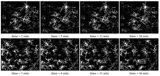
Figure 8.
Reconstruction results of 3D microglia images over time. The video of the reconstruction results for the top and bottom rows could be found in Supplementary Information materials SI2 and SI4, respectively.
We measure consistency over consecutive time frames by calculating the average of the standard deviation of the measures between each time frame. The consistency results are shown in Figure 9. The five measures describe the differences between the reconstruction results and the baseline result. Therefore, the standard deviation between the measures over time frames show how similar the results are over time. The results from C3VFC, FMST, and MST show a low average standard deviation which constitute to better consistency. FMST and MST results are consistently over segmented which could be a desired attribute.
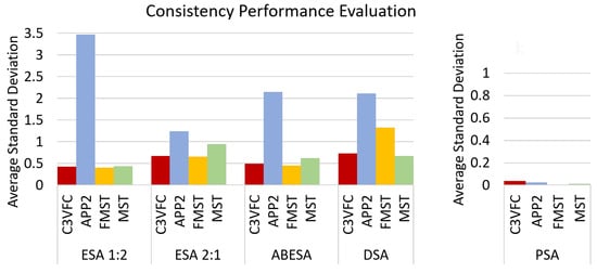
Figure 9.
Consistency measure for the reconstruction results over time. We compare the standard deviations over time of the five performance measures (ESA 1:2, ESA 2:1, ABESA, DSA, and PSA) for each of the reconstruction algorithms (C3VFC, APP2, FMST, and MST). A lower average standard deviation constitutes a more consistent change over time. The scale for the PSA graph is from 0 to 1 because the is a percentage.
4.3. Bioinformatics Analysis
Tracing consistent skeletons over time is a first step in analyzing microglia morphology in different scenarios. There is still much unknown about the role of microglia in different settings, particularly with respect to neurodegenerative disease. It is known that the morphology and motility of microglia changes in these diseased states. This section describes how our temporal tracing result from C3VFC can be used to analyze the dynamic behavior of glial cells.
In [52], the authors developed a ramification index to explain changes in microglia motility when microglia activation is inhibited. Their ramification index was a measure of the ratio of the cell’s perimeter over its area and normalized to a circle of that area: . If R=1, then the cell has no branches, and thus no ramification. This ramification index was used for the 2D maximum intensity projection of the image. From this, we develop a 3D ramification index that can also describe the changes in extension and retraction of the microglia processes in different settings. Our 3D territorial ramification index (TRI) is a measure of the ratio of the volume of the convex hull of the skeleton and the volume of the soma. The convex hull is a polygonal enclosure of the extension of the skeleton. The TRI measures the ramification of the cell as a whole. As seen in Figure 10, the processes of the microglia start to retract and then extends over time.
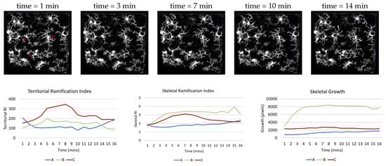
Figure 10.
The top row frames of a video with microglia in motion after a laser burn induced injury, explained in Section 3.2. The video depicting the top row can be found in supplementary materials that is labeled SI4. The graphs show the associated measures over time for three microglia labeled in the first image.
We also develop the skeletal ramification index which puts more weight on the individual branches. The SRI is the ratio of the volume of the skeleton and the volume of the soma. indicates no ramification. From Figure 10, the cell labeled B may cover less territorial volume than glia C, but there is greater branch growth.
From Figure 11, we show the TRI and SRI of five different microglia. The figure exemplifies that the soma size effects the TRI and SRI indexes since it is normalized by the soma volume.
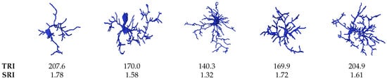
Figure 11.
Examples of the TRI and SRI measures with different microglia.
Lastly, we measure the skeletal growth by finding the skeletal volume over time. The skeletal volume is computed by counting the total number of voxels in the skeleton and subtracting the soma volume. The soma has such a large volume compared to the thinned processes that it would outweigh the effects of the process volume. Additionally, this skeletal growth represents how the processes are surveilling its environment over time. The slope of this line is the velocity that measures how fast the skeleton changes over time.
4.4. Representing Microglia as Graphs
C3VFC is an automatic tracing algorithm that detects the cells in an image, traces the branches back to the soma, and also converts the tracing into a graph for bioinformatics analysis. Microglia comprises of a soma and processes that extends from it. This cell structure could be represented as a tree, or an acyclic undirected graph [53,54]. An acyclic graph is a graph with no loops. An undirected graph contains edges with no direction. Our method represents each foreground pixel in the traced skeleton as a vertex and is connected by an edge link, with a weight value of the Euclidean distance between connected pixels, where the graph is defined as . We use the mathematical tree representation of the microglia to acquire structure information and complexity analysis of the cell structure. A bifurcation is when the path divides into two parts. In microglia, the ramification and addition of new processes over time is telling of its environment. Microglia are highly ramified as it is surveying its surroundings. However, the processes are less ramified, with less bifurcations, in a diseased setting, as described in Section 1.
Figure 12 depicts a microglia represented as a tree, with a different color constituting a different hierarchy of the paths. The path hierarchy of a vertex is defined in [55] as the number of bifurcations that is crossed when traversed back to the root node or the soma. The paths closest to the root node will have a value of one and the hierarchy number increases with more bifurcations.
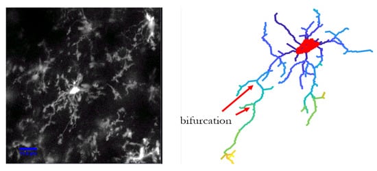
Figure 12.
The path hierarchy is depicted by the different colors. The paths hierarchy at each node is determined by the number of bifurcations that are crossed when traversed back to the soma.
5. Discussion
In this paper, we propose the C3VFC algorithm for tracing and labeling 3D multi-cellular images of glia over consecutive time frames. In summary, the method followed the sequential steps: Soma detection, critical point detection, and centerline tracing. C3VFC utilizes vector field convolution in conjunction with constrained concentric circles to easily find the critical points that lie in the centerline of the glia processes. The critical points are traversed back to the corresponding soma to trace the glia processes. The output of the algorithm is the microglia reconstructions of a multi-cellular image that is labeled over time frames. The labeled reconstruction results could be individually analyzed over time in a SWC format. We proved the efficacy of the reconstruction results with bioinformatics we developed to explain motility and morphology changes of microglia which can be used to analyze cells in different environments. The bioinformatics we provided included two ramification indexes, a skeletal growth index, and structural graph representation. Our contributions for a microglia reconstruction algorithm and accompanying bioinformatics were motivated by its desire in current literature and our collaborators in the neuroscience field.
In the experiments, we proved significant accuracy results and consistency in the C3VFC reconstruction results over consecutive time frames. We used datasets of 3D multi-cellular microglia images over 16 time frames. These 3D muli-cellular images over time were input into the C3VFC algorithm, while the individual cells had to be manually cropped before inputting them into the state-of-the-art methods that were used for comparison. Even so, in all of our experiments, C3VFC achieved a significantly higher accuracy measure to the manual baseline than all other methods in , , ABESA, DSA, and PDS. We define significant as having a lower difference measure than the next best score. We generated the highest accuracy on the temporal microglia datasets, with up to 53% improvement over the next best reconstruction result. We also test the consistency of the reconstruction results to prove that C3VFC consistently achieves accurate results for all five measures over time frames. This proves that C3VFC could correctly trace the centerline and achieve better reconstruction results. We also proved the efficacy of our workflow since the microglia reconstructions were labeled over time, showing that dynamic bioinformatics could be extracted.
There are some limitations to C3VFC. In 3D images, portions of the cell could exist outside of the field of view. A sufficient amount of erroneous tracing of branches happen in cases where the soma body of a cell is outside the field of view but the processes are in the field of view. Still, C3VFC produces consistent tracing results of multiple microglia in the field of view over time frames that are easily manipulated for extracting bioinformatics.
Supplementary Materials
The following are available online at https://www.mdpi.com/article/10.3390/app11136078/s1, Video S1: C3VFC reconstruction result, Video S2: C3VFC reconstruction result, Video S3: C3VFC reconstruction result, Video S4: C3VFC reconstruction result from mouse with laser-induced burn.
Author Contributions
Conceptualization, T.T.L. and J.W.; methodology, T.T.L.; image acquisition, K.B. and U.E.; software, T.T.L.; validation, T.T.L.; formal analysis, T.T.L.; investigation, T.T.L.; resources, T.T.L.; data curation, T.T.L.; writing—original draft preparation, T.T.L.; writing—review and editing, T.T.L., J.W. and S.T.A.; visualization, T.T.L.; supervision, S.T.A.; project administration, S.T.A.; funding acquisition, S.T.A. All authors have read and agreed to the published version of the manuscript.
Funding
This research was funded by National Science Foundation under grant number 1759802. Any opinions, findings, and conclusions or recommendations expressed in this material are those of the authors and do not necessarily reflect the views of the National Science Foundation.
Institutional Review Board Statement
Not applicable.
Acknowledgments
We would also like to thank Samantha Batista and Tajie Harris in the Harris lab at UVa for the single cell image acquisition and Harris’ continual mentorship. We would like to acknowledge Dan Weller for his continual guidance on this project.
Conflicts of Interest
The authors declare no conflict of interest.
References
- Lucin, K.M.; Wyss-Coray, T. Immune activation in brain aging and neurodegeneration: Too much or too little? Neuron 2009, 64, 110–122. [Google Scholar] [CrossRef]
- Eyo, U.B.; Wu, L.J. Bidirectional microglia-neuron communication in the healthy brain. Neural Plast. 2013, 2013, 456857. [Google Scholar] [CrossRef]
- Colonna, M.; Butovsky, O. Microglia function in the central nervous system during health and neurodegeneration. Annu. Rev. Immunol. 2017, 35, 441–468. [Google Scholar] [CrossRef] [PubMed]
- Schafer, D.P.; Stevens, B. Microglia function in central nervous system development and plasticity. Cold Spring Harb. Perspect. Biol. 2015, 7, a020545. [Google Scholar] [CrossRef] [PubMed]
- Poliani, P.L.; Wang, Y.; Fontana, E.; Robinette, M.L.; Yamanishi, Y.; Gilfillan, S.; Colonna, M. TREM2 sustains microglial expansion during aging and response to demyelination. J. Clin. Investig. 2015, 125, 2161–2170. [Google Scholar] [CrossRef]
- Cronk, J.C.; Filiano, A.J.; Louveau, A.; Marin, I.; Marsh, R.; Ji, E.; Goldman, D.H.; Smirnov, I.; Geraci, N.; Acton, S.; et al. Peripherally derived macrophages can engraft the brain independent of irradiation and maintain an identity distinct from microglia. J. Exp. Med. 2018, 215, 1627–1647. [Google Scholar] [CrossRef] [PubMed]
- Wake, H.; Moorhouse, A.J.; Jinno, S.; Kohsaka, S.; Nabekura, J. Resting microglia directly monitor the functional state of synapses in vivo and determine the fate of ischemic terminals. J. Neurosci. 2009, 29, 3974–3980. [Google Scholar] [CrossRef] [PubMed]
- Tremblay, M.È.; Lowery, R.L.; Majewska, A.K. Microglial interactions with synapses are modulated by visual experience. PLoS Biol. 2010, 8, e1000527. [Google Scholar] [CrossRef]
- Davalos, D.; Ryu, J.K.; Merlini, M.; Baeten, K.M.; Le Moan, N.; Petersen, M.A.; Deerinck, T.J.; Smirnoff, D.S.; Bedard, C.; Hakozaki, H.; et al. Fibrinogen-induced perivascular microglial clustering is required for the development of axonal damage in neuroinflammation. Nat. Commun. 2012, 3, 1227. [Google Scholar] [CrossRef]
- Ginhoux, F.; Lim, S.; Hoeffel, G.; Low, D.; Huber, T. Origin and differentiation of microglia. Front. Cell. Neurosci. 2013, 7, 45. [Google Scholar] [CrossRef]
- Hristovska, I.; Pascual, O. Deciphering resting microglial morphology and process motility from a synaptic prospect. Front. Integr. Neurosci. 2016, 9, 73. [Google Scholar] [CrossRef]
- Madry, C.; Kyrargyri, V.; Arancibia-Cárcamo, I.L.; Jolivet, R.; Kohsaka, S.; Bryan, R.M.; Attwell, D. Microglial ramification, surveillance, and interleukin-1β release are regulated by the two-pore domain K+ channel THIK-1. Neuron 2017, 97, 299–312.e6. [Google Scholar] [CrossRef]
- Savage, J.C.; Carrier, M.; Tremblay, M.È. Morphology of microglia across contexts of health and disease. Microglia 2019, 2034, 13–26. [Google Scholar]
- Au, N.P.B.; Ma, C.H.E. Recent advances in the study of bipolar/rod-shaped microglia and their roles in neurodegeneration. Front. Aging Neurosci. 2017, 9, 128. [Google Scholar] [CrossRef]
- Nimmerjahn, A.; Kirchhoff, F.; Helmchen, F. Resting microglial cells are highly dynamic surveillants of brain parenchyma in vivo. Science 2005, 308, 1314–1318. [Google Scholar] [CrossRef] [PubMed]
- Wu, L.J.; Zhuo, M. Resting microglial motility is independent of synaptic plasticity in mammalian brain. J. Neurophysiol. 2008, 99, 2026–2032. [Google Scholar] [CrossRef] [PubMed]
- Davalos, D.; Grutzendler, J.; Yang, G.; Kim, J.V.; Zuo, Y.; Jung, S.; Littman, D.R.; Dustin, M.L.; Gan, W.B. ATP mediates rapid microglial response to local brain injury in vivo. Nat. Neurosci. 2005, 8, 752. [Google Scholar] [CrossRef]
- Morrison, H.W.; Filosa, J.A. A quantitative spatiotemporal analysis of microglia morphology during ischemic stroke and reperfusion. J. Neuroinflammation 2013, 10, 1–20. [Google Scholar] [CrossRef] [PubMed]
- York, E.M.; LeDue, J.M.; Bernier, L.P.; MacVicar, B.A. 3DMorph automatic analysis of microglial morphology in three dimensions from ex vivo and in vivo imaging. Eneuro 2018, 5. [Google Scholar] [CrossRef]
- Abdolhoseini, M.; Kluge, M.G.; Walker, F.R.; Johnson, S.J. Segmentation, tracing, and quantification of microglial cells from 3D image stacks. Sci. Rep. 2019, 9, 1–10. [Google Scholar] [CrossRef]
- Wang, Y.; Narayanaswamy, A.; Tsai, C.L.; Roysam, B. A broadly applicable 3-D neuron tracing method based on open-curve snake. Neuroinformatics 2011, 9, 193–217. [Google Scholar] [CrossRef]
- Wang, Y.; Narayanaswamy, A.; Roysam, B. Novel 4-D open-curve active contour and curve completion approach for automated tree structure extraction. Proceedings of CVPR 2011, IEEE, Colorado Springs, CO, USA, 20–25 June 2011; pp. 1105–1112. [Google Scholar]
- Yuan, X.; Trachtenberg, J.T.; Potter, S.M.; Roysam, B. MDL constrained 3-D grayscale skeletonization algorithm for automated extraction of dendrites and spines from fluorescence confocal images. Neuroinformatics 2009, 7, 213–232. [Google Scholar] [CrossRef] [PubMed]
- Levit, C.; Lasinski, T. A tool for visualizing the topology of three-dimensional vector fields. In Proceedings Visualization’91; Citeseer: Washington, DC, USA, 1991; pp. 33–40. [Google Scholar]
- Malcolm, N.O.; Popelier, P.L. An improved algorithm to locate critical points in a 3D scalar field as implemented in the program MORPHY. J. Comput. Chem. 2003, 24, 437–442. [Google Scholar] [CrossRef]
- Xie, J.; Zhao, T.; Lee, T.; Myers, E.; Peng, H. Anisotropic path searching for automatic neuron reconstruction. Med. Image Anal. 2011, 15, 680–689. [Google Scholar] [CrossRef]
- Wan, Z.; He, Y.; Hao, M.; Yang, J.; Zhong, N. M-AMST: An automatic 3D neuron tracing method based on mean shift and adapted minimum spanning tree. BMC Bioinform. 2017, 18, 1–13. [Google Scholar] [CrossRef][Green Version]
- Yang, J.; Hao, M.; Liu, X.; Wan, Z.; Zhong, N.; Peng, H. FMST: An automatic neuron tracing method based on fast marching and minimum spanning tree. Neuroinformatics 2019, 17, 185–196. [Google Scholar] [CrossRef] [PubMed]
- Sofka, M.; Stewart, C.V. Retinal vessel centerline extraction using multiscale matched filters, confidence and edge measures. IEEE Trans. Med Imaging 2006, 25, 1531–1546. [Google Scholar] [CrossRef] [PubMed]
- Mukherjee, S.; Condron, B.; Acton, S.T. Tubularity flow field—A technique for automatic neuron segmentation. IEEE Trans. Image Process. 2015, 24, 374–389. [Google Scholar] [CrossRef]
- Ly, T.; Thompson, J.; Harris, T.; Acton, S.T. The Coupled TuFF-BFF Algorithm for Automatic 3D Segmentation of Microglia. In Proceedings of the 2018 25th IEEE International Conference on Image Processing (ICIP), Athens, Greece, 7–10 October 2018; IEEE: Piscataway, NJ, USA, 2018; pp. 121–125. [Google Scholar]
- Li, B.; Acton, S.T. Active contour external force using vector field convolution for image segmentation. IEEE Trans. Image Process. 2007, 16, 2096–2106. [Google Scholar] [CrossRef]
- Mukherjee, S.; Acton, S.T. Vector field convolution medialness applied to neuron tracing. In Proceedings of the 2013 IEEE International Conference on Image Processing, Melbourne, Victoria, 15–18 September 2013; IEEE: Piscataway, NJ, USA, 2013; pp. 665–669. [Google Scholar]
- Basu, S.; Aksel, A.; Condron, B.; Acton, S.T. Segmentation and tracing of neurons in 3D. IEEE Trans. Inf. Tech. Biomed. 2012, 17, 319–335. [Google Scholar]
- Mukherjee, S.; Basu, S.; Condron, B.; Acton, S.T. Tree2Tree2: Neuron tracing in 3D. In Proceedings of the Biomedical Imaging (ISBI), 2013 IEEE 10th International Symposium on IEEE, San Francisco, CA, USA, 7–11 April 2013; pp. 448–451. [Google Scholar]
- Xiao, Z.; Ni, J.; Liu, Q.; Jiang, L.; Wang, X. Study on automatic tracking algorithm of neurons in most atlas of mouse brain based on open curve snake. In Proceedings of the 2017 IEEE 4th International Conference on Soft Computing & Machine Intelligence (ISCMI), IEEE, Mauritius, 23–24 November 2017; pp. 140–144. [Google Scholar]
- Sui, D.; Wang, K.; Zhang, Y.; Zhang, H. A novel seeding method based on spatial sliding volume filter for neuron reconstruction. In Proceedings of the 2013 IEEE International Conference on Bioinformatics and Biomedicine, Shanghai, China, 18–21 December 2013; IEEE: Piscataway, NJ, USA, 2013; pp. 29–34. [Google Scholar]
- Sui, D.; Wang, K.; Chae, J.; Zhang, Y.; Zhang, H. A pipeline for neuron reconstruction based on spatial sliding volume filter seeding. Comput. Math. Methods Med. 2014, 2014, 386974. [Google Scholar] [CrossRef] [PubMed]
- Bisht, K.; Sharma, K.; Eyo, U.B. Precise Brain Mapping to Perform Repetitive In Vivo Imaging of Neuro-Immune Dynamics in Mice. JOVE J. Vis. Exp. 2020. [Google Scholar] [CrossRef] [PubMed]
- Yona, S.; Kim, K.W.; Wolf, Y.; Mildner, A.; Varol, D.; Breker, M.; Strauss-Ayali, D.; Viukov, S.; Guilliams, M.; Misharin, A.; et al. Fate mapping reveals origins and dynamics of monocytes and tissue macrophages under homeostasis. Immunity 2013, 38, 79–91. [Google Scholar] [CrossRef]
- Madisen, L.; Zwingman, T.A.; Sunkin, S.M.; Oh, S.W.; Zariwala, H.A.; Gu, H.; Ng, L.L.; Palmiter, R.D.; Hawrylycz, M.J.; Jones, A.R.; et al. A robust and high-throughput Cre reporting and characterization system for the whole mouse brain. Nat. Neurosci. 2010, 13, 133. [Google Scholar] [CrossRef] [PubMed]
- Jan-Kroon, D. Comprehensive Meta-Analysis; Hessian Based Frangi Vesselness Filter, MATLAB Central File Exchange: New York, NY, USA, 2021. [Google Scholar]
- Frangi, A.F.; Niessen, W.J.; Vincken, K.L.; Viergever, M.A. Multiscale vessel enhancement filtering. In International Conference on Medical Image Computing and Computer-Assisted Intervention; Springer: Berlin/Heidelberg, Germany, 1998; pp. 130–137. [Google Scholar]
- Hassouna, M.S.; Farag, A.A. Multistencils fast marching methods: A highly accurate solution to the eikonal equation on cartesian domains. IEEE Trans. Pattern Anal. Mach. Intell. 2007, 29, 1563–1574. [Google Scholar] [CrossRef] [PubMed]
- Stockley, E.; Cole, H.; Brown, A.; Wheal, H. A system for quantitative morphological measurement and electrotonic modelling of neurons: Three-dimensional reconstruction. J. Neurosci. Methods 1993, 47, 39–51. [Google Scholar] [CrossRef]
- Xiao, H.; Peng, H. APP2: Automatic tracing of 3D neuron morphology based on hierarchical pruning of a gray-weighted image distance-tree. Bioinformatics 2013, 29, 1448–1454. [Google Scholar] [CrossRef]
- Peng, H.; Ruan, Z.; Long, F.; Simpson, J.H.; Myers, E.W. V3D enables real-time 3D visualization and quantitative analysis of large-scale biological image data sets. Nat. Biotechnol. 2010, 28, 348–353. [Google Scholar] [CrossRef]
- Peng, H.; Bria, A.; Zhou, Z.; Iannello, G.; Long, F. Extensible visualization and analysis for multidimensional images using Vaa3D. Nat. Protoc. 2014, 9, 193–208. [Google Scholar] [CrossRef] [PubMed]
- Peng, H.; Tang, J.; Xiao, H.; Bria, A.; Zhou, J.; Butler, V.; Zhou, Z.; Gonzalez-Bellido, P.T.; Oh, S.W.; Chen, J.; et al. Virtual finger boosts three-dimensional imaging and microsurgery as well as terabyte volume image visualization and analysis. Nat. Commun. 2014, 5, 1–13. [Google Scholar] [CrossRef]
- Bria, A.; Iannello, G.; Onofri, L.; Peng, H. TeraFly: Real-time three-dimensional visualization and annotation of terabytes of multidimensional volumetric images. Nat. Methods 2016, 13, 192–194. [Google Scholar] [CrossRef]
- Longair, M.H.; Baker, D.A.; Armstrong, J.D. Simple Neurite Tracer: Open source software for reconstruction, visualization and analysis of neuronal processes. Bioinformatics 2011, 27, 2453–2454. [Google Scholar] [CrossRef] [PubMed]
- Bryan, R.M.; Attwell, D. Microglial Ramification, Surveillance, and Interleukin-1b Release Are Regulated by the Two-Pore Domain K Channel THIK-1. Neuron 2018, 97, 1–14. [Google Scholar]
- Batabyal, T.; Acton, S.T. Elastic path2path: Automated morphological classification of neurons by elastic path matching. In Proceedings of the 2018 25th IEEE International Conference on Image Processing (ICIP), Athens, Greece, 7–10 October 2018; IEEE: Piscataway, NJ, USA, 2018; pp. 166–170. [Google Scholar]
- Ly, T.T.; Batabyal, T.; Thompson, J.; Harris, T.; Weller, D.S.; Acton, S.T. Hieroglyph: Hierarchical Glia Graph Skeletonization and Matching. In Proceedings of the Asilomar Conference on Signals, Systems and Computers, Pacific Grove, CA, USA, 30 March 2020. [Google Scholar]
- Basu, S.; Condron, B.; Acton, S.T. Path2Path: Hierarchical path-based analysis for neuron matching. In Proceedings of the 2011 IEEE International Symposium on Biomedical Imaging: From Nano to Macro, Chicago, IL, USA, 30 March–2 April 2011; IEEE: Piscataway, NJ, USA, 2011; pp. 996–999. [Google Scholar]
Publisher’s Note: MDPI stays neutral with regard to jurisdictional claims in published maps and institutional affiliations. |
© 2021 by the authors. Licensee MDPI, Basel, Switzerland. This article is an open access article distributed under the terms and conditions of the Creative Commons Attribution (CC BY) license (https://creativecommons.org/licenses/by/4.0/).